Stochastic description of geometric phase for polarized waves in random media

Abstract

We present a stochastic description of multiple scattering of polarized waves in the regime of forward scattering. In this regime, if the source is polarized, polarization survives along a few transport mean free paths, making it possible to measure an outgoing polarization distribution. We solve the direct problem using compound Poisson processes on the rotation group $SO(3)$ and non-commutative harmonic analysis. The obtained solution generalizes previous works in multiple scattering theory and is used to design an algorithm solving the inverse problem of estimating the scattering properties of the medium from the observations. This technique applies to thin disordered layers, spatially fluctuating media and multiple scattering systems and is based on the polarization but not on the signal amplitude. We suggest that it can be used as a non invasive testing method.

1 Introduction

Soon after its discovery in adiabatic quantum systems by Berry [3], experimental evidence of a geometric phase for polarized light travelling along a bended optical fiber was shown by Tomita and Chiao [23]. It was rapidly realized that any classical transverse polarized wave could exhibit a geometric phase [22] when travelling along a curved path in a three dimensions space. This, however, is only possible if the wave remains polarized, and if the direction of propagation evolves smoothly with time.

If one emits a plane monochromatic wave into a scattering medium, the multiple scattering events will result in a spreading of the distribution of the wave vector with time [25]. Depending on the strength and density of the scatterers, this spreading will happen at different rates. The correlation length of the wave vector is called the transport mean free path $\ell^{\star}$. It is directly related, in the multiple scattering regime, to the effective diffusion constant of the energy in the system $D=c\ell^{\star}/3$ [19] ($c$ is the velocity of the wave). Several multiple scattering regimes exist, depending on the ratio between the wavelength $\lambda$, the size $a$ of the scatterers, the mean free path $\ell$, the transport mean free path $\ell^{\star}$ and the depth of the medium $L$ [9]. In this article, we will investigate the regime

$$\lambda<a\ll\ell\ll\ell^{\star}\lesssim L.$$ (1)

The condition $\ell\ll\ell^{\star}$ states that the wave is preferentially scattered to a direction close to the incoming one. This is the so called “forward scattering” regime. For spherical scatterers, this is a consequence of the condition $\lambda<a$.

The transport mean free path $\ell^{\star}$ is the length scale of disorder in the medium while the transport mean free path is the scale along which the waves behave as homogeneous. Measuring the transport mean free path is therefore an important issue in experiments because it is the resolution scale for most of the physical quantities measurable using waves. Several estimation techniques already exist for the transport mean free path that can be distinguished from the direction of the measured signal. The simplest idea is to use the intensity transmission ratio [7] to measure $\ell^{\star}$ thanks to the diffusion approximation. Diffusion models are also useful in anisotropic media [10] and to describe intensity leaks in direction orthogonal to the incoming source [14]. In backscattering setup, the opening angle of the weak localization cone, in which an intensity enhancement due to interferences is observed, is related to the transport mean free path in the medium [24]. All these experiments rely on intensity measurements. An amplitude independent method has been proposed to measure the mean free path $\ell$ from the phase statistics of a Gaussian field [1].

It is known that in the forward scattering regime polarization is parallel transported during the propagation, which may result in the existence of a geometric phase [15]. In the eikonal approximation, each ray possesses a geometric phase depending on its geometry. At a given point, the observed phase is not uniquely defined, but has a distribution related to the distribution of paths from the source. This distribution was recently shown to depend on the outgoing direction of the ray [20].

The distribution of geometric phase from multiple scattering of a polarized incident wave was adressed ten years ago [12] without any condition on the final direction. The calculation was based on Brownian motion at the surface of a sphere and followed an approach developed earlier by Antoine et al. [2]. However multiple scattering is rigorously a Brownian motion on a sphere only in the limit of very weak and dense scatterers. A more general model would be a random walk with macroscopic steps.

We consider media with a thickness $L$ of the order of a few $\ell^{\star}$, therefore the outgoing wave vectors are not evenly distributed. The joint distribution of direction and polarization state, related to paths statistics, contains informations concerning the scattering events that are not yet randomized. The number of scattering events is of the order of $L/\ell$ and in the case where this number is not very large ($L/\ell\simeq 10$) the usual approximations are not suited. For this reason, attention was recently brought to stochastic processes for the description of a scattering system where the number of scattering events is small.

Stochastic models have been introduced fifteen years ago in multiple scattering [16] to solve direct problems. Recently, Le Bihan and Margerin [13] showed that a stochastic model for the direction of propagation can be used to solve inverse problems. They computed the mean free path in a medium from the distribution of outgoing directions. We extend this model to take polarization into account and estimate the transport mean free path $\ell^{\star}$ from the geometric phase distribution.

2 Scattering of polarized waves

Without loss of generality, we consider linearly polarized waves. The results we present remain valid as long as polarization is not purely circular.

Polarization of transverse waves lies in the plane orthogonal to the direction of propagation. We describe linearly polarized plane waves with two vectors: The direction of propagation ${\boldsymbol{k}}$ and the direction of polarization $\boldsymbol{p}$, with $\boldsymbol{p}\perp{\boldsymbol{k}}$. We consider only media with isotropic uniform absorption, the wave amplitude is therefore completely determined for all paths and does not play any relevant role. The direction ${\boldsymbol{k}}$ lies on the unit sphere $\mathcal{S}^{2}\subset{\mathbf{R}}^{3}$. The direction of polarization $\boldsymbol{p}$ lies in the tangent plane $T_{\boldsymbol{k}}\mathcal{S}^{2}$. The frame $\mathit{F}$ is fully determined by ${\boldsymbol{k}}$ and $\boldsymbol{p}$ and contains all information concerning the polarization and direction of propagation. (The third vector of $\mathit{F}$ is indeed ${\boldsymbol{k}}\times\boldsymbol{p}$).

We follow the wave state along a ray using the frame $\mathit{F}$. Between scattering events, $\mathit{F}$ remains constant. The changes of $\mathit{F}$ occur at scattering events. As $\mathit{F}$ is a frame, any change, or jump, of $\mathit{F}$ corresponds to a rotation matrix. The scattering angle $\theta$ is random, following a probability distribution function (pdf) called phase function $\Phi(\theta)$ that depends on $a/\lambda$ and on the nature of the scatterer. The average value of $\left\langle\cos\theta\right\rangle=\int\Phi(\theta)\cos\theta\sin\theta\mathrm{d}\theta$ is called the scattering anisotropy and is noted $g$. In the forward scattering regime, the main scattering angle $\theta$ is small and $g$ is close to $1$. We use the ZYZ convention for the Euler angles describing the rotations of $SO(3)$ and note the angles $(\psi,\theta,\varphi)\in\left]-\pi,\pi\right]\times\left]0,\pi\right]\times\left]-\pi,\pi\right]$.

The rotation matrix $\mathrm{P}$ acting on the frame $\mathit{F}$ at a scattering event is fully determined by the incoming direction ${\boldsymbol{k}}$ and the outgoing direction ${\boldsymbol{k}}^{\prime}$ and the requirement that the vector $\boldsymbol{p}$ is parallel transported [15]. On the unit sphere, jumps of the stochastic process are represented by geodesics (arcs of great circles). Moreover, parallel transport in the direct space implies parallel transport in the phase space from $T_{\boldsymbol{k}}\mathcal{S}^{2}$ to $T_{{\boldsymbol{k}}^{\prime}}\mathcal{S}^{2}$ [11] and therefore that the angle between $\boldsymbol{p}$ and the geodesic remains constant. As a consequence the Euler angles $\psi$ and $\varphi$ of the rotation matrix $\mathrm{P}$ are related by (see figure 1)

$$\psi=-\varphi.$$ (2)

Parallel transport of polarization through a scattering event may therefore be described by a rotation matrix $\mathrm{P}(\theta,\psi)$, $\theta$ is the length of the geodesic on the unit sphere and $\psi$ is the angle between this geodesic and the polarization vector $\boldsymbol{p}$. The relation between the incoming and outgoing frames is

$$\mathit{F}^{\prime}=\mathit{F}\,\mathrm{P}\left(\theta,\,\psi\right).$$ (3)

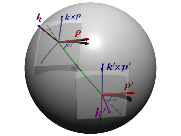
Figure 1: Parallel transport of a vector along the geodesic of length $\theta$ (solid line). The parallel transport constraint results in the fact that $\psi$ and $\varphi$ are equal (algebrically opposite).

Note that the rotation matrix $\mathrm{P}$ acts on the right of $\mathit{F}$. An expression in terms of left action of rotation matrices can be obtained, but would lead to a random process over $SO(3)$ with dependent increments. The independence of increments will be useful for the repeated action (3) on $\mathit{F}$ that we present in the next section.

3 Multiple scattering process

We consider a plane wave with linear polarization, corresponding to the frame $\mathit{F}_{0}$ as described in the previous section. The scattering events are described as random rotations acting on the right of $\mathit{F}_{0}$. The frame $\mathit{F}_{0}$ changes according to Equation (3) for each scaterring event, so that it becomes the frame $\mathit{F}_{n}$ after $n$ scattering events:

$$\mathit{F}_{n}=\mathit{F}_{0}\mathrm{P}\left(\theta_{1},\,\psi_{1}\right)\mathrm{P}\left(\theta_{2},\,\psi_{2}\right)\cdots\mathrm{P}\left(\theta_{n},\,\psi_{n}\right).$$ (4)

The scattering event are independent and the scatterers are identical, so that the random rotations $\mathrm{P}\left(\theta_{m},\,\psi_{m}\right)$ are independent and identically distributed.

From the source to the observer, a wave may encounter a variable number of scatterers. The number of scattering events in a time $t$ can be taken as a Poisson process $N(t)$ [13]. The Poisson parameter $\eta$ is directed related to the mean free path $\ell$ by $\eta=c/\ell$. All these considerations result in the process $\mathit{F}_{t}$ which we define as

$$\mathit{F}_{t}=\mathit{F}_{0}\prod_{k=1}^{N(t)}\mathrm{P}\left(\theta_{k},\,\psi_{k}\right),$$ (5)

where $\displaystyle{\prod}$ denotes the right-sided product on $SO(3)$. This equation expresses the stochastic process $\mathit{F}_{t}$ as a compound Poisson process (CPP) on $SO(3)$ with parallel transport. We denote by $p_{\nu}$ the distribution of the process $\mathit{F}_{t}$ at a given time $t$, with $\nu=\eta t$. A Poisson process is a pure jump process with independent increments and we have

$$p_{\nu}=\sum_{n=0}^{\infty}\mathrm{e}^{-\nu}\,\frac{\nu^{n}}{n!}\;p_{\mathit{F}_{n}}.$$ (6)

where $\mathrm{e}^{-\nu}\frac{\nu^{n}}{n!}$ is the probability to have exactly $n$ scattering events in the time interval $[0,t]$. Thanks to Equation (4) and the independence of the parallel transport rotations, $p_{\mathit{F}_{n}}$ is given by [4]:

$$p_{\mathit{F}_{n}}=p_{\mathit{F}_{0}}\ast p_{\mathrm{P}_{1}}\ast\cdots\ast p_{\mathrm{P}_{n}}=\Phi^{\ast[n]}.$$ (7)

Here the symbol $\ast$ is the convolution product on $SO(3)$ and $\Phi^{\ast[n]}$ denotes the result of the convolution of $n$ identical functions $\Phi$. We have used the initial condition $p_{\mathit{F}_{0}}=\delta\left(I_{3}-\mathit{F}_{0}\right)$. In the case where the source is a distribution of directions of propagation and polarization, the distribution $p_{\mathit{F}_{n}}$ is the convolution of the initial distribution $p_{\mathit{F}_{0}}$ with $\Phi^{\ast[n]}$.

4 Harmonic analysis

We use harmonic analysis on $SO(3)$ to transform the expression (7). Harmonic analysis on $SO(3)$ is similar to Fourier series and in particular transforms convolutions into products. As in Ref. [13], we get a semi-analytic expression of $p_{\nu}$ that we use for statistical estimation in Section 5.

Th Fourier basis of functions $f\in L^{2}(SO(3),{\mathbf{R}})$ is made of the Wigner $D$-matrices $(D^{j})_{j\geqslant 0}$ [6, 4]. The Wigner $D$-matrices are $(2j+1)\times(2j+1)$ square matrices with coefficients

$$D^{j}_{m,n}(\psi,\theta,\,\varphi)=\mathrm{e}^{-\mathrm{i}m\psi}d^{j}_{m,n}(\theta)\mathrm{e}^{-\mathrm{i}n\varphi}.$$ (8)

The Fourier coefficients are matrices of the same size which coefficients are defined as $\widetilde{f}^{j}_{m,n}=\left\langle\Phi\mid D^{j}_{m,n}\right\rangle$, where $\langle\;\rangle$ represents the scalar product for function on $SO(3)$ [6]. Like in the circular Fourier theory, the transform of a convolution is a product (here, a matrix product)

$$\widetilde{f_{1}\ast f_{2}}^{j}=\widetilde{f_{1}}^{j}\widetilde{f_{2}}^{j}.$$ (9)

We deduce the Fourier coefficients of $p_{\nu}$ from Equation (6)

$$\widetilde{p_{\nu}}^{j}=\sum_{n=0}^{\infty}\mathrm{e}^{-\nu}\frac{\nu^{n}}{n!}\left(\widetilde{\Phi}^{j}\right)^{n}=\exp\left[\nu(\widetilde{\Phi}^{j}-I_{2j+1})\right],$$ (10)

where $\exp$ denotes the matrix exponential. Using the notation $\Delta(x)=2\pi\sum_{k}\delta(x-2\pi k)$ to put the parallel transport constraint on the Fourier coefficients we obtain

$$\widetilde{\Phi}^{j}_{m,n}=\frac{1}{8\pi^{2}}\iiint\Phi(\theta)\Delta(\varphi+\psi)D^{j}_{m,n}(\psi,\,\theta,\,\varphi)\sin\theta\mathrm{d}\theta\,\mathrm{d}\varphi\,\mathrm{d}\psi.$$ (11)

We can simplify using the definition (8)

$$\widetilde{\Phi}^{j}_{m,n}=\frac{\delta_{mn}}{2}\int_{0}^{\pi}\Phi(\theta)d^{j}_{m,m}(\theta)\sin\theta\mathrm{d}\theta,$$ (12)

and show that the Fourier matrices $\widetilde{\Phi}^{j}$ are diagonal for all $j$. Thanks to Equation (10), it is clear that $\widetilde{p_{\nu}}^{j}$ is also diagonal at all orders $j$.

Using the inverse Fourier formula [6], $p_{\nu}$ reads:

$$p_{\nu}=\frac{1}{2\pi}\sum_{j=0}^{\infty}(2j+1)\operatorname{Tr}(\widetilde{p_{\nu}}^{j}D^{j\dagger})$$ (13)

where $\operatorname{Tr}$ denotes the trace and the ^† denotes the Hermitian conjugation of elements from $\mathcal{M}_{2j+1}(\mathbf{C})$.

The variable $\beta=\psi-\varphi$ represents the direction of polarization of the wave after its propagation through the medium, which is the geometric phase. Thanks to symmetry, the distribution of $\beta$ is the same as the one of $\psi+\varphi$. Combined with the fact that $\widetilde{p_{\nu}}^{j}$ is diagonal, we conclude that $p_{\nu}$ is a function of $\theta$ and $\beta$

$$p_{\nu}(\theta,\,\beta)=R_{0}(\theta,\,\nu)+2\sum_{m\geq 1}\cos(m\beta)R_{m}(\theta,\,\nu),$$ (14)

$$R_{m}(\theta,\,\nu)=\frac{1}{2\pi}\sum_{j\geq m}(2j+1)\mathrm{e}^{\nu(\widetilde{\Phi}^{j}_{m,m}-1)}d^{j}_{m,m}(\theta).$$ (15)

Thus, Equation (14) is a general expression of the distribution of geometric phase in multiple scattering regime for polarized waves. We have only assumed that the scatterers are spherical and identical.

The limit of Brownian motion, which is made of isotropic infinitesimal steps of spherical length $\delta$ occuring at a large rate $\eta$, corresponds to the physical situation where scatterers are very weak but have a large spatial density. For a single step, we get $\tilde{\Phi}^{j}_{m,m}=\exp[-\frac{1}{2}j(j+1)\delta^{2}]$. Taking the limit $\delta\to 0$ and $\eta\to\infty$ such that $\delta^{2}\nu=\delta^{2}\eta t=Dt$ remains constant, formula (14) gives the distribution of the geometric phase for a wave propagating in a heterogeneous continuous medium. In formula (14), one should replace $\nu(\tilde{\Phi}^{j}_{m,m}-1)$ by $-\frac{1}{2}j(j+1)Dt$. This formula was demonstrated by Perrin in his study of rotational Brownian motion [17, 18], while computing the distribution of $\varphi+\psi$.

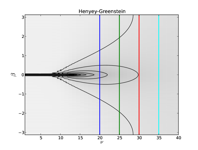
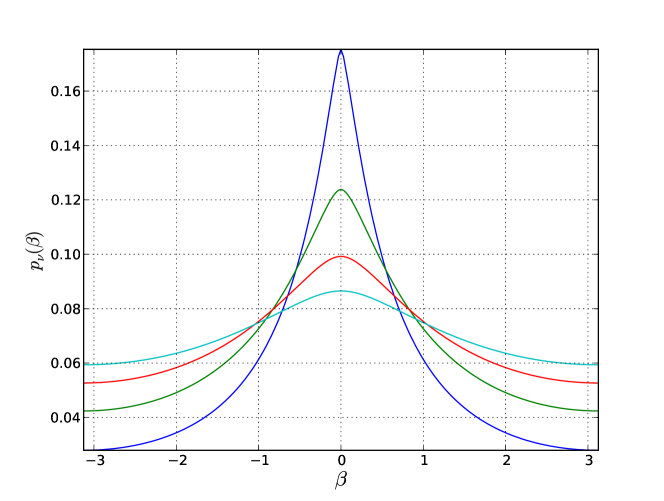
Figure 2: Evolution of the density $(p_{\eta t}(\theta=0,\,\beta)$ with time in a medium containing Henyey-Greenstein scatterers with anisotropy $g=0.8$. The curves are iso-density levels from $0.05$ to $0.45$ by increments of $0.05$. The vertical lines correspond to the slices displayed on Figure 3.

Figure 3: Distribution of the geometric phase $\beta$ for the values of the Poisson parameter $\nu=\eta t$ : $\nu=20$, $\nu=25$, $\nu=30$ and $\nu=35$. corresponding to the vertical lines of Figure 3.

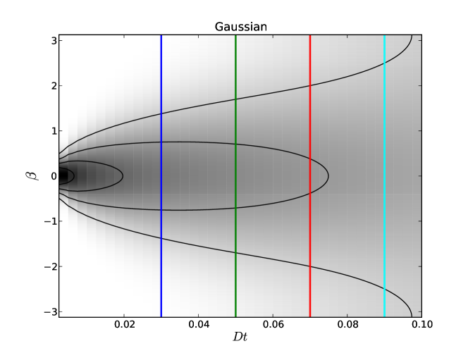
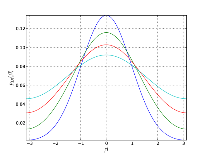
Figure 4: Evolution of the density $p_{Dt}(\theta=0,\,\beta)$ with time for a Gaussian phase function. This corresponds to the rotational Brownian motion on the sphere studied by Perrin in Ref. [18]. The curves are iso-density levels from $0.05$ to $0.45$ by increments of $0.05$. The vertical lines correspond to the slices displayed on Figure 5.

Figure 5: Density $p_{Dt}(\theta=0,\,\beta)$ for a Gaussian phase function with the values $Dt=0.03$, $Dt=0.05$, $Dt=0.07$ and $Dt=0.09$ corresponding to the vertical lines of Figure 5.

Taking $\theta=0$ in Equation (14) we get the result demonstrated by Antoine et al. [2], and integrating over $\theta$ we find the result obtained by Krishna et al. [12] up to a small difference, ($j(j+1)$ has to be replaced by $j(j+1)-m^{2}$). Equation (14) is therefore a generalization of these known formulas that can be applied to an arbitrary phase function, also in the case of a small number of scattering events and for an arbitrary deviation angle $\theta$. The origin of the small difference comes from the fact that the Brownian motion of the tangent vector of a particle moving in space $\mathbf{R}^{3}$ has one more degree of freedom than the Brownian motion on $\mathcal{S}^{2}$ (the rotation degree of freedom about the tangent vector). In References [2, 12] the extra degree of freedom disappears because these authors considered rotations with $\psi=0$ and in this work, we considered rotations with $\varphi+\psi=0$. Let us remark that the set of these latter rotations forms a group but that the set of rotations with $\psi=0$ does not.

We display the distribution obtained from formula (14) in the two following cases: discrete Henyey-Greenstein scatterers with anisotropy $g=0.8$ on a range of Poisson parameter up to $\nu=20$ on the one hand (Figures 3 and 3) and diffusive limit with $D=1\;\mathrm{rad^{2}\,s^{-1}}$ on the other hand (Figures 5 and 5). The exit angle is $\theta=0$ for all of the figures. We can observe that the behavior of the distributions on Figures 3 and 5 are very different, especially at short times, the distribution $p_{\nu}$ is sharply peeked for the Henyey-Greenstein scatterers but in the case of Brownian motion it is smooth. At long times, depolarization is observed in both cases. The depolarized state is reached with significantly distinct behaviours. This is an illustration that depolarization is significantly dependent on the scattering properties of the medium. It is therefore natural to investigate how these scattering properties can be estimated from observations through signal analysis.

We have shown that the polarization distribution depends on the angle between the outgoing wave vector ${\boldsymbol{k}}_{\text{out}}$ and the initial one ${\boldsymbol{k}}_{0}$. Moreover, it actually depends on the position of the last scattering event. Let us call $\chi$ the angle coordinate of this point in the cylindrical coordinates of axis ${\boldsymbol{k}}_{0}$ in the frame $\mathit{F}_{0}$, and $(\theta,\,\phi)$ the spherical coordinates of ${\boldsymbol{k}}_{\text{out}}$ in the same frame. The distribution of polarization is then the one given by formula (14) shifted by an angle $(1-\cos\theta)\chi$. This shift is due to the fact that the reference $\beta=0$ is taken in the parallel transported frame from the source to the last scattering event, so that an extra phase appears in the frame $\mathit{F}_{0}$. This extra phase has been already observed in backscattering configuration ($\theta=\pi$) [8, 21].

We remark that in the case where $\tilde{\Phi}^{j}_{m,m}$ depends only on $j$ (and is noted $\tilde{\Phi}^{j}$), formula (14) simplifies to

$$p_{\nu}(\theta,\beta)=\sum_{j\geqslant 0}(2j+1)\mathrm{e}^{\nu(\tilde{\Phi}^{j}-1)}\frac{\sin\left(j+\frac{1}{2}\right)\omega}{\sin\frac{1}{2}\omega},$$ (16)

with $\cos\frac{\omega}{2}=\cos\frac{\theta}{2}\cos\frac{\beta}{2}$. As a consequence, there is an unexpected symmetry for $p_{\nu}$ between the outgoing angle and the geometric phase.

5 Inverse problem

In this section, we take advantage of the Fourier expansion and propose a statistical estimation of the mean free path $\ell$ obtained from the measured distribution of the geometric phase $\beta$. This is achieved by estimating the Poisson parameter $\nu=\eta t$. The estimate of $\nu$ is denoted by $\hat{\nu}$.

The inverse problem is solved using an expectation-minimization (EM) approach [5] with the parametric CPP. The EM algorithm is based on the maximization of the log-likelihood of the a posteriori distribution given in Equation (6). Suppose that we are given a sample of size $M$ of observations (measurements) $\mathit{F}_{m}$, $1\leqslant m\leqslant M$. We assume that each observation $\mathit{F}_{m}$ follows independently the probability law (14), the joint probability distribution function is simply the product $\prod_{m}p_{\nu}(\mathit{F}_{m})$, with $p_{\nu}(\mathit{F})=p_{\nu}(\theta,\psi+\varphi)$, where $\varphi$, $\theta$ and $\psi$ are the Euler angles of $\mathit{F}$. The value of $\nu$ that maximizes this log-likelihood is

$$\hat{\nu}=\operatorname*{arg\,max}_{\nu}\left(\sum_{m=1}^{M}\log p_{\nu}(\mathit{F}_{m})\right).$$ (17)

The EM algorithm is an iterative procedure that almost surely converges to a local minimum [5]. The minimization step (M-step) consists in updating the estimate $\hat{\nu}$, while the expectation step (E-step) consists in updating $\mathbb{P}\left(n\mid\mathit{F},\,\hat{\nu}_{i}\right)=p_{\mathit{F}_{n}}(\mathit{F})/p_{\hat{\nu}_{i}}(\mathit{F})\times\mathrm{e}^{-\hat{\nu}_{i}}\hat{\nu}_{i}^{n}/n!$. We get a sequence of estimates with the relation

$$\hat{\nu}_{i+1}=\frac{1}{M}\sum_{m=1}^{M}\frac{1}{p_{\hat{\nu}_{i}}(\mathit{F}_{m})}\sum_{n=0}^{\infty}n\,p_{\mathit{F}_{n}}(\mathit{F}_{m})\,\mathrm{e}^{-\hat{\nu}_{i}}\,\frac{\hat{\nu}_{i}^{n}}{n!}.$$ (18)

In practice the sums over $n$ in Equation (18) and Equation (6) and over $j$ in Equation (15) are truncated to an arbitrarily fixed value $N$. At most $N$ scattering events are described by the model, therefore $N$ should be taken large compared to $L/\ell$. This EM-algorithm is able to estimate one parameter, the Poisson parameter $\nu$ (or equivalently the mean free path $\ell=ct/\nu$), which means that we have considered that the phase function $\Phi$ is known. It is nonetheless possible to estimate simultaneously any finite number of parameters of $p_{\nu}$, such as the anisotropy $g$ of the scatterers, but the iteration formulas are more sophisticated.

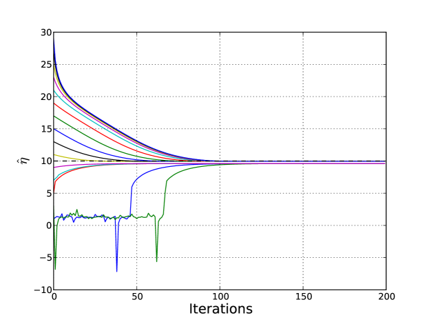
Figure 6: Convergence of the estimate of the Poisson parameter $\hat{\eta}_{i}$ using EM algorithm with different initialization values ranging from $1$ to $29$. The actual value of $\eta$ was set to $10$.

We illustrate the behaviour of the EM algorithm in Figure 6 which shows the convergence of the estimator $\hat{\nu}$ for different initial values $\hat{\nu}_{0}$. Acceleration procedures could be developped in the case of large dataset from experimental setup. Note that no local minima were reached in the simulation, leading to convergence in all the cases. However, as can be seen for initial values inferior to $10$ in Figure 6, underestimated initial values lead to a systematic bias in $\hat{\nu}$. This suggests that high values should be privileged when processing dataset, as it does not penalize convergence and leads to a more accurate estimate.

6 Conclusions

The description of the depolarization of multiply scattered waves can be made, in the forward scattering regime, through a compound Poisson process (CPP). This stochastic model predicts the distribution of the geometric phase in all directions, for discrete or continuous scattering media. generalizing existing results (forward outgoing direction or a spatially fluctuating medium). Moreover, the CPP model allows a more detailed description of the phenomenon as it provides the behaviour of this distribution as a function of the output scattering angle $\theta$. The present approach allows to design an iterative procedure to estimate properties of the scattering medium through the measurement of the outgoing polarization distribution. We have illustrated this point by presenting an expectation-minimization (EM) algorithm for the estimation of the Poisson parameter, which is directly linked to the transport mean free path $\ell^{\star}$. An interesting feature of this technique is that is relies on polarization rather than on amplitude measurements. Future work will consist in validating the proposed model and estimation algorithm on measurement of polarization distribution for real experiment.

Acknoledgments

This work was founded by the CNRS/PEPS grant PANH.

References

References

- [1] D. Anache-Ménier, B. A. van Tiggelen, and L. Margerin, Phase statistics of seismic coda waves, Phys. Rev. Lett. 102 (2009), 248501.
- [2] Michel Antoine, Alain Comtet, Jean Desbois, and Stéphane Ouvry, Magnetic fields and Brownian motion on the 2-sphere, J. Phys. A: Math. Gen. 24 (1991), 2581–2586.
- [3] M. V. Berry, Quantal phase factors accompanying adiabatic changes, Proc. R. Soc. A 392 (1984), 45–57.
- [4] G.S. Chirikjian and A.B. Kyatkin, Engineering applications of noncommutative harmonic analysis, CRC Press, 2001.
- [5] A.P. Dempster, D.B. Laird, and D.B. Rubin, Maximum likelihood from incomplete data via the EM algorithm, Journal of the royal statistical society, Series B 39 (1977), no. 1, 1–38.
- [6] J. Dieudonné, Special functions and linear representations of lie groups, American Mathematical Society, 1980.
- [7] N. Garcia, A. Z. Genack, and A. A. Lisyansky, Measurement of the transport mean free path of diffusing photons, Phys. Rev. B 46 (1992), 14475–14478.
- [8] Andreas H. Hielscher, Angela A. Eick, Judith R. Mourant, Dan Shen, James P. Freyer, and Irving J. Bigio, Diffusive backscattering mueller matrices of highly scattering media, Opt. Expr. 1 (1997), 441–453.
- [9] A. Ishimaru, Wave propagation and scattering in random media, vol.1,2, Academic Press, New York, 1978.
- [10] P. M. Johnson, Sanli Faez, and Ad Lagendijk, Full characterization of anisotropic diffuse light, Optics Express 16 (2008), 7435–7446.
- [11] T. F. Jordan and J. Maps, Change of the plane of oscillation of a Foucault pendulum from simple pictures, Am. J. Phys. 78 (2010), 1188.
- [12] M.M.G. Krishna, J. Samuel, and S. Sinha, Brownian motion on a sphere: distribution of solid angles, J. Phys. A: Math. Gen. 33 (2000), 5965.
- [13] Nicolas Le Bihan and Ludovic Margerin, Nonparametric estimation of the heterogeneity of a random medium using compound Poisson process modeling of wave multiple scattering, Phys. Rev. E 80 (2009), 016601.
- [14] Marco Leonetti and Cefe López, Measurement of transport mean-free path of light in thin systems, Opt. Letters 36 (2011), 2824–2826.
- [15] A. C. Maggs and V. Rossetto, Writhing photons and Berry phases in polarized multiple scattering, Phys. Rev. Lett. 87 (2001), 253901.
- [16] X. Ning, L. Papiez, and G. Sandison, Compound-Poisson-process method for the multiple scattering of charged particles, Phys. Rev. E 52 (1995), no. 5, 5621–5633.
- [17] Francis Perrin, Étude mathématique du mouvement brownien de rotation, Ann. Éc. Norm 45 (1928), 1–51.
- [18] , Mouvement browien d’un ellipsoïde (II), J. Phys. Radium 1 (1936), 1–11.
- [19] David J. Pine, D. A. Weitz, P. M. Chaikin, and E. Herbolzheimer, Diffusing-wave spectroscopy, Phys. Rev. Lett. 60 (1988), 1134–1137.
- [20] Vincent Rossetto, A general framework for multiple scattering of polarized waves including anisotropies and Berry phase, Phys. Rev. E 80 (2009), 056605.
- [21] Vincent Rossetto and A. C. Maggs, Writhing geometry of stiff polymers and scattered light, Eur. Phys. J. B 118 (2002), 323–326.
- [22] Jan Segert, Photon Berry’s phase as a classical topological effect, Phys. Rev. A 36 (1987), 10–15.
- [23] Akira Tomita and Raymond Y. Chiao, Observation of Berry’s topological phase by use of an optical fiber, Phys. Rev. Lett. 57 (1986), 937–940.
- [24] Meint P. Van Albada and Ad Lagendijk, Observation of weak localization of light in a random medium, Phys. Rev. Lett. 24 (1985), 2692–2695.
- [25] H. C. van de Hulst, Light scattering by small particles, Dover, 1957.