COOPERATION ON SOCIAL NETWORKS
AND ITS ROBUSTNESS

Abstract

In this work we have used computer models of social-like networks to show by extensive numerical simulations that cooperation in evolutionary games can emerge and be stable on this class of networks. The amounts of cooperation reached are at least as much as in scale-free networks but here the population model is more realistic. Cooperation is robust with respect to different strategy update rules, population dynamics, and payoff computation. Only when straight average payoff is used or there is high strategy or network noise does cooperation decrease in all games and disappear in the Prisoner’s Dilemma.

1 Introduction

Game theory is used in many contexts, particularly in economy, biology, and social sciences to describe situations in which the choices of the interacting agents are interdependent. Evolutionary game theory in particular is well suited to the study of strategic interactions in animal and human populations and has a well defined mathematical structure that allows analytical conclusions to be reached in the context of well-mixed and very large populations (see e.g. [33, 8]). However, starting with the works of Axelrod [3], and Nowak and May [19] population structures with local interactions have been brought to the focus of research since they are supposed to be closer model of real social structures. Indeed, social interactions can be more precisely represented as networks of contacts in which nodes represent agents and links stand for their relationships. Thus, in the wake of the flurry of research on complex networks [18], evolutionary game theory has been recently enhanced with networked population structures. The corresponding literature has already grown to a point that makes it difficult to be exhaustive; however, good recent reviews can be found in [27, 22, 20]. In particular, the problems of cooperation and coordination, leading to social efficiency problems and social dilemmas, have been studied in great detail through some well known paradigmatic games such as the Prisoner’s Dilemma, Snowdrift, and the Stag Hunt. Those games, although unrealistic with respect to actual complex human behavior, constitute a simple way for gaining a basic understanding of these important issues. One of the important findings in this line of research is that the heterogeneous structure of many model and actual networks may favor the evolution of socially valuable equilibria, for instance leading to non-negligible amounts of cooperation in a game such as the Prisoner’s Dilemma where the theoretical result should be generalized defection [23, 26, 22]. Coordination on the socially preferable Pareto-efficient equilibrium in the Stag Hunt and an increase of the fraction of cooperators in the Snowdrift game have also been observed on populations interacting according to a complex network structure [26, 22].

Most detailed results on evolutionary games on networks to date have been obtained for network types that are standard in graph theory such as Erdös-Rényi random graphs, scale-free networks, Watts–Strogatz small-world networks, and a few others that are commonly used (see [22] for a good complete review). This is obviously an important first step, since general results have been obtained for these network topologies, especially through numerical simulations and in some cases even analytical ones [27]. However, since the theory is of interest especially when applied in human or animal societies, to move a further step on, the network structures used should be as close as possible to those that can be observed in such contexts. This is the realm of social networks, many of which have been investigated and their main statistics established (see, for instance, [18]). While social networks degree distributions have been found to be broad-scale in general and thus they share this property [1], at least in part, with model scale-free networks they also possess some features that are not found in most common model networks. The three more important for our purposes are: clustering, positive degree assortativity, and community structure [16, 18]. Thus, in the present study we would like to offer a rather systematic study of evolutionary games played on this kind of networks in order to pave the way for the understanding of their behavior in real societies. Actually, there have already been several studies of evolutionary games on particular social networks in the past (see, for example and among others, [9, 12, 13]). Broadly speaking, these investigations all tend to show that socially valuable outcomes such as cooperation and coordination are more likely to evolve than in unstructured populations. However, the particular nature of the few networks used, although it provides some insight, does not allow one to draw more general and statistically valid conclusions. For this reason, here, instead of studying another particular network, we prefer to follow the methodology used in investigations such as [26, 22], where numerical simulation results are validated by using many runs on different networks belonging to the same class. As a model for constructing social networks, among several different possibilities, we choose to use Toivonen et al.’s model [30], which will be discussed in Sect. 4. This model has already been investigated in [13], albeit for a different evolution rule and for a reduced game phase space. In this paper, in addition to numerically studying the steady states of evolutionary games on these social network models when using static networks and error-free strategy update rules, we shall also briefly explore the effect of errors on strategy update rules and noise on network structure.

The paper is organized as follows. We first present some background on two-person, two-strategies symmetric games, followed by evolutionary games on networks. This is followed by a description of the model networks used. Next, results for the chosen games are presented and discussed, as well as the effects induced by the introduction of noise. We then offer our conclusions and some ideas for future work.

2 Games Studied

We have studied the four classical two-person, two-strategies symmetric games described by the generic payoff bi-matrix of Table 1.

$\begin{array}[]{c|cc}&C&D\\ \hline\cr C&(R,R)&(S,T)\\ D&(T,S)&(P,P)\end{array}$

Table 1: Generic payoff bi-matrix for the two-person, two-strategies symmetric games. $C$ and $D$ are the possible strategies, and $R,T,P$, and $S$ are utility values as discussed in the text.

In this matrix, $R$ stands for the reward the two players receive if they both cooperate ($C$), $P$ is the punishment for bilateral defection ($D$), and $T$ is the temptation, i.e. the payoff that a player receives if she defects while the other cooperates. In the latter case, the cooperator gets the sucker’s payoff $S$. Payoff values may undergo any affine transformation without affecting neither the Nash equilibria, nor the dynamical fixed points; however, the parameters’ values are restricted to the “standard” configuration space defined by $R=1$, $P=0$, $-1\leq S\leq 1$, and $0\leq T\leq 2$. In the resulting $TS$ plane, each game’s space corresponds to a different quadrant depending on the ordering of the payoffs.

If the payoff values are ordered such that $T>R>P>S$ then defection is always the best rational individual choice, so that $(D,D)$ is the unique Nash Equilibrium (NE) and also the only Evolutionarily Stable Strategy (ESS) [33]. This famous game is called Prisoner’s Dilemma (PD). Mutual cooperation would be socially preferable but $C$ is strongly dominated by $D$.

In the Snowdrift (SD) game, the order of $P$ and $S$ is reversed, yielding $T>R>S>P$. Thus, in the SD when both players defect they each get the lowest payoff. $(C,D)$ and $(D,C)$ are NE of the game in pure strategies. There is a third equilibrium in mixed strategies which is the only dynamically stable state, while the two pure NE are not [33]. Players have a strong incentive to play $D$, which is harmful for both parties if the outcome produced happens to be $(D,D)$.

With the ordering $R>T>P>S$ we get the Stag Hunt (SH) game in which mutual cooperation $(C,C)$ is the best outcome, Pareto-superior, and a NE. The second NE, where both players defect is less efficient but also less risky. The dilemma is represented by the fact that the socially preferable coordinated equilibrium $(C,C)$ might be missed for “fear” that the other player will play $D$ instead. The third mixed-strategy NE in the game is evolutionarily unstable [33].

Finally, the Harmony game has $R>S>T>P$ or $R>T>S>P$. $C$ strongly dominates $D$ and the trivial unique NE is $(C,C)$. This game is non-conflictual by definition and does not cause any dilemma: it is included just to complete the quadrants of the parameter space.

With the above conventions, in the figures that follow, the PD space is the lower right quadrant; the SH is the lower left quadrant, and the SD is in the upper right one. Harmony is represented by the upper left quadrant.

3 Evolutionary Games on Networks

In this section we present background material on evolutionary games on finite-size populations of agents represented by networks of contacts to make the paper as self-contained as possible.

3.1 Population structure

The population of players is represented by a connected unweighted, undirected graph $G(V,E)$, where the set of vertices $V$ represents the agents, while the set of edges $E$ represents their symmetric interactions. The population size $N$ is $|V]$, the cardinality of $V$. The set of neighbors of an agent $i$ is defined as: $V_{i}=\{j\in V\>|\>\mathit{dist}(i,j)=1\}$, and its cardinality $|V_{i}|$ is the degree $k_{i}$ of vertex $i\in V$. The average degree of the network is called $\bar{k}$ and $P(k)$ denotes its degree distribution function, i.e. the probability that an arbitrarily chosen node has degree $k$. The network topologies used are explained in Sect. 4.

3.2 Payoff calculation and strategy revision rules

In evolutionary game theory, one must specify how individual’s payoffs are computed and how agents revise their present strategy. In the standard theory, there is a very large well-mixed population; however, when the model is applied to a finite population whose members are the vertices of a graph, each agent $i$ can only interact with agents contained in the neighborhood $V_{i}$, i.e. only local interactions are permitted.

Let $s_{i}\in\{C,D\}$ be the current strategy of player $i$ and let us call $M$ the payoff matrix of the game. The quantity

$$\Pi_{i}(t)=\sum_{j\in V_{i}}\sigma_{i}(t)\;M\;\sigma_{j}^{T}(t)$$

is the accumulated payoff collected by agent $i$ at time step $t$ and $\sigma_{i}(t)$ is a vector giving the strategy profile at time $t$ with $C=(1\;\;0)$ and $D=(0\;\;1)$. We also use the average payoff $\overline{\Pi}_{i}(t)$ defined as the average of accumulated payoff collected by a given agent $i$ at time step $t$:

$$\overline{\Pi}_{i}(t)=\frac{1}{k_{i}}\>\sum_{j\in V_{i}}\sigma_{i}(t)\;M\;\sigma_{j}^{T}(t)$$

Several strategy update rules are commonly used. Here we shall describe three rules belonging to the imitative class that have been used in our simulations; the first rule is deterministic, while the following strategy updates are stochastic.

The first rule is to switch to the strategy of the neighbor that has scored best in the last time step. This imitation of the best policy can be described in the following way: the strategy $s_{i}(t)$ of individual $i$ at time step $t$ will be

$$s_{i}(t)=s_{j}(t-1),$$

where

$$j\in\{V_{i}\cup i\}\;s.t.\;\Pi_{j}=\max\{\Pi_{k}(t-1)\},\;\forall k\in\{V_{i}\cup i\}.$$

That is, individual $i$ will adopt the strategy of the player with the highest payoff among its neighbors including itself. If there is a tie, the winner individual is chosen uniformly at random, but otherwise the rule is deterministic.

The local replicator dynamics rule is stochastic [7]. Player $i$’s strategy $s_{i}$ is updated by drawing another player $j$ from the neighborhood $V_{i}$ with uniform probability, and replacing $s_{i}$ by $s_{j}$ with probability:

$$p(s_{i}\rightarrow s_{j})=(\Pi_{j}-\Pi_{i})/K,$$

if $\Pi_{j}>\Pi_{i}$, and keeping the same strategy if $\Pi_{j}\leq\Pi_{i}$. $K=\max(k_{i},k_{j})[(\max(1,T)-\min(0,S)]$, with $k_{i}$ and $k_{j}$ being the degrees of nodes $i$ and $j$ respectively, ensures proper normalization of the probability $p(s_{i}\rightarrow s_{j})$.

The last strategy revision rule is the Fermi rule [27]:

$$p(s_{i}\rightarrow s_{j})=\frac{1}{1+\exp(-\beta(\Pi_{j}-\Pi_{i}))}.$$

This gives the probability that player $i$ switches from strategy $s_{i}$ to $s_{j}$, where $j$ is a randomly chosen neighbor of $i$. $\Pi_{j}-\Pi_{i}$ is the difference of payoffs earned by $j$ and $i$ respectively. The parameter $\beta$ in the function gives the amount of noise: a low $\beta$ corresponds to high probability of error and, conversely, high $\beta$ means low error rates. This interpretation comes from physics, where the reciprocal of $\beta$ is called the temperature. Consequently, payoffs will be more noisy as temperature is raised ($\beta$ is lowered). In the above expressions we have used the accumulated payoff $\Pi_{i}$. Analogous formulae hold for average payoff $\overline{\Pi}_{i}$.

3.3 Strategy update timing

Usually, agents systems in evolutionary game theory are updated synchronously. However, strictly speaking, simultaneous update is physically unfeasible as it would require a global clock, while real extended systems in biology and society in general have to take into account finite signal propagation speed. Furthermore, simultaneity may cause some artificial effects in the dynamics which are not observed in real systems [10]. However, for evolutionary game theory on networks the common wisdom is that the timing of updates does not influence the system properties in a fundamental manner and results are similar in most cases [22, 6], with asynchronism being sometimes beneficial to the emergence of cooperation [6]. This is called an elementary time step. To compare synchronous and asynchronous dynamics, here we use the customary fully asynchronous update, i.e. updating a randomly chosen agent at a time with replacement. The two dynamics, synchronous and fully asynchronous are the extremes cases. It is also possible to update the agents in a partially synchronous manner where a fraction $f=n/N$ of randomly chosen agents is updated in each time step. When $n=N$ we recover the fully synchronous update, while $n=1$ gives the extreme case of the fully asynchronous update. Varying $f$ thus allows one to investigate the role of the update policy on the dynamics [21, 6].

3.4 Simulation parameters

The networks used in all simulations are of size $N=4000$ with mean degree $\bar{k}=8$. The $TS$ plane has been sampled with a grid step of $0.05$ and each value in the phase space reported in the figures is the average of $100$ independent runs, using a fresh graph realization for each run. The initial graph for each run doesn’t change in the static case, while it evolves in the dynamic case, as described in the main text. Note that steady states have always been reached when strategies evolve on a static graph. In the asynchronous dynamics, we first let the system evolve for a transient period of $4000\times N\simeq 16\times 10^{6}$ elementary time steps. In the synchronous case, the same total number of updates is performed. The averages are calculated at the steady state that is reached after the transient period. True equilibrium states in the sense of stochastic stability are not guaranteed to be reached by the simulated dynamics. For this reason we prefer to use the terms steady states which are configurations that have little or no fluctuation over an extended period of time. In the case of fluctuating networks, the system as a whole never reaches a steady state in the sense specified above. This is due to the fact that the link dynamics remains always active. However, the distribution of strategies on the network does converge to a state that shows little fluctuation, i.e. a steady state.

4 Network Construction and Properties

Figure 1: Cumulated degree distribution of a TSN compared with a standard Barabási–Albert network of the same size and mean degree (see text).

There exist several models for constructing social-like networks [29]. Among them, we have chosen Toivonen et al.’s model [30], called here the Toivonen Social Network (TSN), which was conceived to construct a network with most of the desired features of real-life social networks i.e., assortativity, high clustering coefficient, community structure, having an adjustable decay rate of the degree distribution, and a finite cut-off. The TSN construction and properties are described in detail in [30]. The process we have used to obtain a TSN can be summarized as follows:

1. Start with a small clique formed by $m_{0}$ vertices.

2. A new vertex $v$ is added to the network and it is connected to $m_{r}$ vertices chosen with uniform probability in the existing network. (random attachment)

3. Vertex $v$ is connected to $m_{s}$ vertices chosen with uniform probability within the list of neighbors of its neighbors. (implicit preferential attachment)
   Every time that vertex $v$ is connected to a new vertex the list of neighbors of its neighbors is updated.

4. Repeat step 2 and 3 until the network has grown to desired size $N$.

Notice that the process responsible for the appearance of high clustering and community structures is step 3. Moreover, this model is slightly different from the original one, because in the latter the list of neighbors in step 3 is not updated as in the former. This modification does not change the original model proprieties.
In the simulations, we have used networks of size $N=4000$ with a clique of $m_{0}=9$ initial nodes as starting network. Every time a new node is added at step 2, its number of initial contacts $m_{r}$ is distributed with probability: $\mathbb{P}(m_{r}=1)=0.5$ and $\mathbb{P}(m_{r}=2)=0.5$, while the number of its secondary contacts $m_{s}$ is uniformly distributed between, and including, the integer values $0$ and $5$. The resulting degree distribution falls below a power law as shown in [30]. The average degree of the network is given by the formula that provides the average degree of a new added vertex:

$$1\cdot\mathbb{P}(m_{r}=1)+2\cdot\mathbb{P}(m_{r}=2)+\sum_{t=0}^{5}t\cdot\mathbb{P}(m_{s}=t)=4$$

Thus, the resulting average degree of the network is $\bar{k}=2\cdot 4=8$.

To compare with another complex network model besides the standard Barabási–Albert (BA) networks [4], we have also used a model proposed by Amaral et al. [1] which also features several of the characteristics of real complex networks, especially the distribution tail cutoff, and takes into account aging and cost constraints in the pure preferential attachment BA model.

In Fig. 1 we depict the degree distribution of a realization of TSN compared with a Barabási–Albert scale-free network, and the Amaral et al. model (in all cases, $N=4000$ and $\bar{k}=8$). The degree distribution of both TSN and the Amaral et al. model falls down faster than in a BA scale-free network and they are in fact closer to a stretched exponential or an exponentially truncated power-law. This agrees with many observations on empirically measured social networks, see e.g. [1, 15, 31].

Table 2 collects a number of statistics on social networks, mainly collaboration networks in various scientific disciplines. These empirical data show that, irrespective of the network size, they are all degree-assortative ($r>0$) and have a high clustering coefficient. These features are shared by TSNs, and partly by the Amaral model, but not by BA networks. Indeed, it has been shown in the literature that most social networks possess these features (for a review, see [16]).

	N	$\bar{k}$	C	r	Ref.
Biology	1 520 251	15.53	0.60	0.127	[16]
Mathematics	253 339	3.92	0.34	0.120	[16]
Physics	52 909	9.27	0.56	0.363	[16]
Computer Science	11 994	2.55	0.50	-	[15]
Genetic Programming (GP)	2 809	4.17	0.66	0.130	[31]
TSN model	4 000	$\sim$ 8.00	0.36	0.123	-
Amaral model	4 000	8.00	0.22	-0.193	-
BA scale-free networks	4 000	8.00	0.01	-0.042	-

Table 2: Some statistical features of model and real networks of coauthorships. $N$ is the network size (number of nodes). Average degree $\bar{k}$; Average clustering coefficient $C=\frac{1}{N}\sum_{j=1,N}C_{i}$, where $C_{i}$ is the node’s individual clustering coefficient [16]; $r$ is the Pearson’s coefficient of neighbors’ degree correlation [16].

Finally, another characteristic feature of most social networks is the presence of communities, i.e. roughly speaking, groups of nodes that are more interconnected in the group than between groups [18]. TSNs do reproduce this feature while models such as the BA do not. For the purpose of illustration only, Fig. 2 shows a small example ($N=500$) of a TSN graph in which communities have been detected using an algorithm based multi-level optimization of modularity [5]. Indeed, its modularity score [17] is $0.544$ confirms the presence of communities, although to assess its statistical significance would require proper comparison with a suitable null model. Amaral model also gives rise to strongly connected clusters of nodes and its modularity is correspondingly very high, about $0.87$.

Figure 2: Community structure in a small TSN ($N=500$).

In conclusion, we shall mainly use the TSN model for generating a family of networks, hoping to be able to reproduce the main features of actual social networks. The Amaral model will also be used in part to compare results of evolutionary games in a couple of more realistic models besides the standard BA one.

5 Results

In this section we report and discuss our simulation results for the $TS$-plane using different strategy update rules, network topology, and evolution dynamics.

5.1 Replicator dynamics

Figure 3 shows average cooperation frequencies for the four games in the case of BA networks (left image), Amaral’s networks (middle), and TSNs (right image). The payoff is accumulated payoff (see Sect. 3.2). For the BA case, the results are very similar to those obtained in [26, 22] for larger systems with the same mean degree. Both visually and from the average game cooperation values shown next to each quadrant, it is clear that TSNs and the Amaral model networks are as favorable to cooperation as the idealized BA case when the strategy update rule is local replicator dynamics. However, the mechanisms responsible for high cooperation seem to be different. While in BA networks highly connected cooperator hubs play the role of catalyzers for the diffusion of the strategy [23], in social-like networks cooperation may thrive thanks to the higher clustering coefficient and the presence of communities. When a local cluster becomes colonized by cooperators, it tends to be robust against attacks by defectors [22].

The results shown are for asynchronous update (see Sect. 3.3), results for the synchronous case are very similar and we do not show them. The results on TSNs also confirm those obtained in [13] where a different update rule and parameter space was used, while the BA case was first shown in [26].

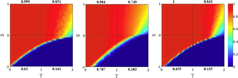
Figure 3: Asymptotic distribution of strategies in the TS plane in BA networks (left), Amaral’s model (middle), and TSNs (right) using replicator dynamics and accumulated payoff. Initial density of cooperators is $0.5$ uniformly distributed at random in all cases. Population evolution is asynchronous. Network size is $N=4000$ and average degree $\bar{k}=8$ in both cases. Values are averages over $100$ independent runs. The numbers in bold next to each quadrant stand for the average cooperation in the corresponding game.

In Fig. 4 we plot average cooperation levels in all games for the case in which agent’s payoffs are averaged over the agent’s links (see Sect. 3.2). As expected, using average payoffs instead of accumulated ones corresponds to make the network more degree-homogeneous and thus the results resemble those obtained in regular random graphs [22] and are similar for both BA networks and TSNs. Defection becomes almost complete in the PD, values are similar to the well-mixed case in the SD, and in the SH the usual bistable result is recovered.

We conclude with [24, 14, 32, 28] that the use of a mean-field for the payoff scheme is detrimental to cooperation. Whether or not this significant factor in social networks is difficult to assess but, obviously, beyond a certain limit, maintaining links becomes expensive in practice and furthermore their frequency of usage should decrease. Probably, real situations are somewhere in between these two extreme cases and thus it is interesting to see what happens when average and accumulated payoff computations both happen to some extent.

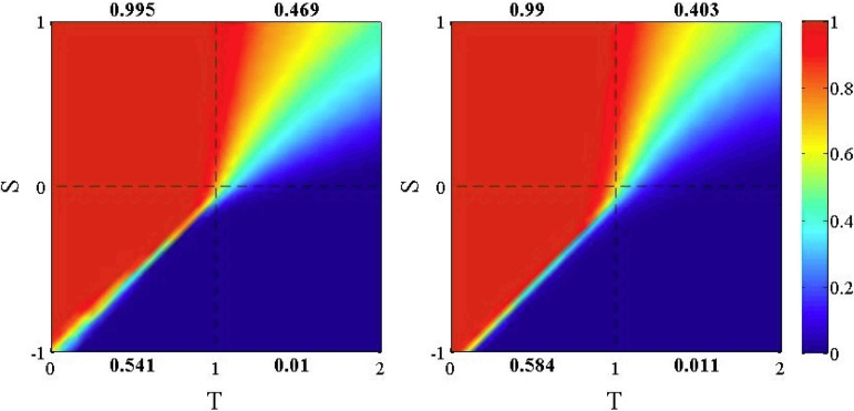
Figure 4: Asymptotic distribution of strategies in the TS plane in BA networks (left) and TSNs (right) using replicator dynamics and average payoff. Initial density of cooperators is $0.5$ uniformly distributed at random in all cases. Network size is $N=4000$ and average degree $\bar{k}=8$ in both cases. Asynchronous population dynamics. Values are averages over $100$ independent runs.

Figure 5: Final average proportion of cooperation in the PD, SD, and SH games as a function of $\alpha$ (see text) for BA and TSN networks. The update is asynchronous and the revision rule is replicator dynamics.

Finally, following the idea of Szolnoki et al. [28], we compute payoffs using a weight parameter $\alpha\in[0,1]$ to represent the proportion of average payoff. Thus, the actual payoff to agent $i$ is given by the formula: $\alpha\overline{\Pi}_{i}+(1-\alpha)\Pi_{i}$. In Fig. 5 we plot the steady-state average cooperation frequency for several $\alpha$ values. Clearly, in all games cooperation decreases with increasing $\alpha$ but the losses are limited in absolute value, except for the SD. Nevertheless, compared with average cooperation at $\alpha=0$, which is $0.135$ for TSN and $0.141$ for BA, the PD looses all residual cooperation.

5.2 Imitation of the best

In this section we compare BA networks with TSNs, and the Amaral model using synchronous and asynchronous population dynamics and the imitation of the best strategy update rule (see Sect. 3.2). The average cooperation results with accumulated payoff are illustrated in Fig. 6. Note that asynchronous dynamics (bottom figures) is more favorable for cooperation in this case for all topologies, as already remarked by Grilo and Correia [6] for the BA case. With this deterministic asynchronous dynamics TNSs are particularly conducive to cooperation, more than $0.5$ in the average for the PD, $0.98$ in the SD phase space, and $0.95$ in the SH quadrant; cooperation is a bit lower for the PD for the Amaral’s case but still good in the whole game phase space. The qualitative reason for the diffusion and stability of cooperation seems to be related to the higher clustering coefficients of TSNs with respect to BA networks (see Table 2). In these networks, if a tightly linked cluster happens to get a large majority of cooperators, it can spread cooperation more easily to next neighbors. This is also true in the synchronous case (top figures) but to a lesser extent for the PD, and almost to the same extent for the SD and the SH, .

Figure 6: Asymptotic distribution of strategies in the TS plane in BA networks (left column), Amaral’s networks (middle), and TSNs (right column) using imitation of the best and accumulated payoff. Top row: synchronous dynamics. Bottom row: asynchronous dynamics. Initial density of cooperators is $0.5$ uniformly distributed at random in all cases. Network size is $N=4000$ and average degree $\bar{k}=8$ in both cases. Values are averages over $100$ independent runs.

The results with average payoff for the BA model and TSNs again with synchronous and asynchronous population dynamics are shown in Fig. 7. The top row shows images for synchronous update in BA networks (left image) and TSNs (right image). When using fully averaged payoffs, the results become similar to those obtained in a regular random graph with the same average degree, as in [22], with a small advantage in cooperation for the TSNs. In the asynchronous case (bottom row) results are similar with somewhat more cooperation in both cases and again an advantage for the TSNs. The results for BA networks have already been obtained by Grilo and Correia and are consistent with ours [6].

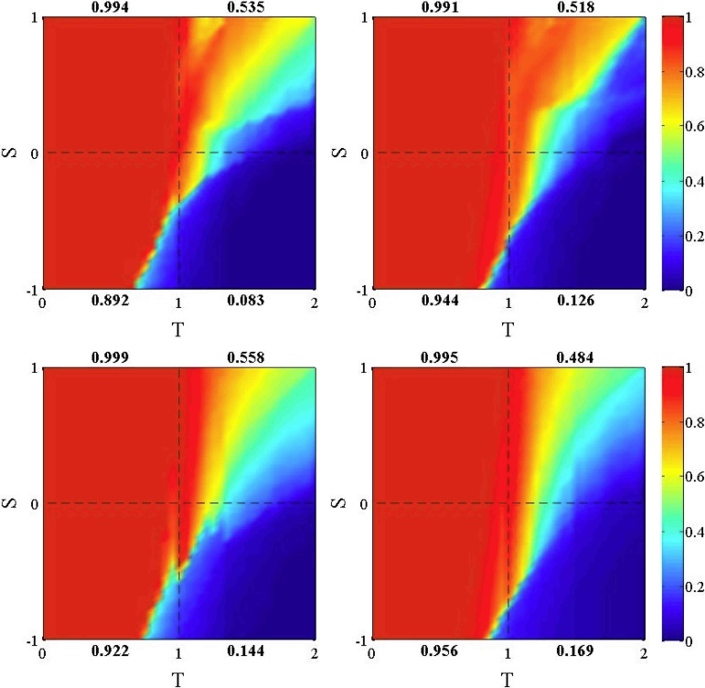
Figure 7: Asymptotic distribution of strategies in the TS plane in BA networks (left column) and TSNs (right column) using imitation of the best and average payoff. Top row: synchronous dynamics. Bottom row: asynchronous dynamics. Initial density of cooperators is $0.5$ uniformly distributed at random in all cases. Network size is $N=4000$ and average degree $\bar{k}=8$ in both cases. Values are averages over $100$ independent runs.

Finally, we present in Fig. 8 the average amount of cooperation for the asynchronous dynamics as a function of the parameter $\alpha$ as explained in the previous section. The most important remark is that cooperation in the TSN model is almost always higher in the whole range of $\alpha$ for all games with respect to BA networks. Concerning the average/accumulated payoff tradeoff, one can see that there is a large decrease of cooperation in the SD and in the PD games going from pure accumulated ($\alpha=0$) to pure average ($\alpha=1$). The SH is less affected.

Figure 8: Final average proportion of cooperation in the PD, SD, and SH games as a function of $\alpha$ (see text) for BA and TSN networks. Population update is asynchronous. The strategy revision rule is imitation of the best.

5.3 Fermi rule

The Fermi strategy update rule allows for the introduction of random noise in the choice of strategy (see Sect. 3.2). In Fig. 9 we show average cooperation results for different $\beta$ values, from left to right $\beta=10,1,0.1,0.01$. The population dynamics is synchronous and thus the results can be compared with the analogous ones obtained by Roca et al. [22] in the case of BA networks. The results are quite similar, with slightly less cooperation in TSNs, and one can see that average cooperation levels tend to decrease with decreasing $\beta$ since this corresponds to increasing randomness in the choice of strategy.

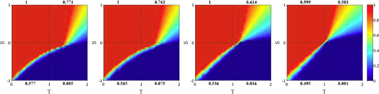
Figure 9: Asymptotic distribution of strategies in the TS plane in TSNs using the Fermi rule with accumulated payoff and synchronous dynamics. Initial density of cooperators is $0.5$ uniformly distributed at random in all cases. Network size is $N=4000$ and average degree $\bar{k}=8$. From left to right: $\beta=10,1,0.1,0.01$. Values are averages over $100$ independent runs.

The asynchronous case is very similar and is not shown to save space. Clearly, those heterogeneous networks make cooperation relatively robust when there is some noise in the choice of strategies, but when the decision becomes almost random topological considerations do not play an important role any longer.

5.4 Network links fluctuations

In a recent study, we have shown by numerical simulations that a certain amount of link rearrangement during evolution may hamper cooperation from emerging in scale-free networks [2]. It is important to note that the dynamics we are referring to is not strategy-related as in other work (see, for instance, [34, 25, 21, 20]); rather, noise is exogenous and random. Under these conditions, we found in [2] that the maintenance of neighborhoods and clusters becomes increasingly difficult with growing noise levels, and this has a negative effect on cooperation. In this section, we shall investigate the same issue for TSNs.

In actual social networks, both the number of links and of nodes tend to increase in time with a speed that is characteristic of a given network, and link formation is not random (see e.g. [11, 31] for two empirical analyses of growing social networks). However, little is known about these complex dynamics and we are not aware of any general theoretical model.

To test for the robustness of cooperation under very simple hypotheses on network fluctuations, and following [2], we have designed a link dynamics well adapted to TSNs through link cutting and rewiring that works as follows:

• a vertex $v$ is chosen uniformly at random in $V$ and its degree $k$ is stored

• cutting edges to neighbors: node $v$ looses all links to its neighbors, except to those that would become isolated by doing so and whose number is $k_{1}$

• relinking node v: vertex $v$ creates $(k-k_{1})$ new links:

  1. node $v$ connects itself uniformly at random with another node $u\notin V_{v}$

  2. vertex $v$ is connected to $4$ vertices chosen with uniform probability within the list of neighbors of its neighbors. Every time that vertex $v$ is connected to a new vertex the list of neighbors of its neighbors is updated

  3. Repeat step 1 and 2 until the number of new links equals $(k-k_{1})$

This kind of rewiring could be interpreted as a sort of migration of node $v$. In the cutting step all of $v$’s previous links are suppressed and the same number of links is created in the relinking step in another region of the network. Vertex $v$ keeps its original degree and thus the mean degree stays constant. If the “moving” node $v$ had neighbors of degree one, those will follow it in the new position to avoid isolated nodes. The degree distribution function changes only slightly, the clustering coefficient remains high, above $0.30$, and the network is always degree-assortative, all of which is consistent with empirical observations on real social networks [11, 31]. Note, however, that our dynamics represents only one among many reasonable possibilities. Reasons of space prevent us from studying other models here.

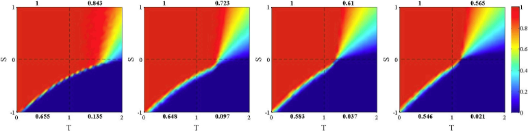
Figure 10: Asymptotic distribution of strategies in the TS plane in TSNs using replicator dynamics with accumulated payoff and asynchronous dynamics. Initial density of cooperators is $0.5$ uniformly distributed at random in all cases. Network size is $N=4000$ and average degree $\bar{k}=8$. From left to right: $\omega=0,10^{-3},10^{-2},2\times 10^{-2}$. Values are averages over $100$ independent runs.

The period of network rewiring is the number of strategy update steps before a node rewiring takes place, and the frequency $\omega$ is just the reciprocal of this number. Figures 10 show average cooperation levels of all games as a function of the rewiring frequency $\omega$. The update rule is replicator dynamics with accumulated payoff and asynchronous population evolution. From left to right: (static case) $\omega=0$, $\omega=10^{-3}$, $\omega=10^{-2}$, $\omega=2\times 10^{-2}$. Values of $\omega$ larger than the latter would cause too fast a rewiring. In actual social networks network dynamics is slow or medium-paced, depending on the type of interaction. The above link dynamics is only intended to qualitatively model those complex phenomena. It is clear that, as in the case of BA networks studied in [2] cooperation is progressively lost with increasing frequency of rewiring $\omega$. This seems to be a general phenomenon in all networks: the loss of cooperation is caused by increasingly fast destruction of an individual’s environment in the network. This noise prevents cooperators from forming stable clusters.

6 Conclusions

In this work we have presented a systematic numerical study of standard two-person evolutionary games on two classes of social network models. The motivation behind this choice is to make a further step towards more realism in the interacting agents population structure. The networks have been built according to Toivonen et al. model (TSN) [30], one of several social network models used in the literature and, in part, according to the model proposed by Amaral et al. [1].

Previous investigations have shown that broad-scale network models such as Barabási–Albert (BA) networks are rather favorable to the emergence of cooperation, with most strategy update rules and using accumulated payoff [23, 26, 22]. Here we have shown that the same is true in general for TSNs and the Amaral model, almost to the same extent as in BA networks. In addition, synchronous and asynchronous population update dynamics have been compared and the positive results remain true and even better for the asynchronous case when using imitation of the best update. We have also presented results for payoff schemes other than accumulated. In particular, we have studied average payoff and various proportions between the two extreme cases. The general observation is that pure average payoff gives the worst results in terms of cooperation, as already noted in [24, 32, 28]. When going from average to accumulate payoff cooperation tends to increase.

Finally, a couple of sources of noise on the evolutionary process have been investigated in order to get an idea about the robustness of cooperation on TSNs. To introduce strategy errors we have used the Fermi update rule. Cooperation on TSNs is relatively robust against this kind of noise, in a manner comparable to scale-free graphs [22]. Of course, when the error rate becomes high, the behavior resembles to random and cooperation tends to decrease for all nontrivial games.

With a view to the fact that actual social networks are never really static, we have designed one among many possible mechanisms to simulate link fluctuations. When this kind of network noise is present cooperation tends to decrease and to disappear altogether when the network dynamics is fast enough. Similar effects have been observed in scale-free networks [2].

In conclusion, TSNs and also Amaral’s networks appear to be as favorable as scale-free graphs for the emergence of cooperation in evolutionary games. But, with respect to the latter, the additional advantages are that TSNs and Amaral networks are much closer to actual social networks in terms of topological structure and statistical features. Cooperation can thus emerge and be stable in this kind of networks and probably also on related models. This is hopefully good news for cooperation among agents in social networks provided that the relationships are sufficiently stable. However, too much strategy noise or network instability may cause cooperation to fade away as in any other network structure.

Acknowledgments.

A. Antonioni and M. Tomassini gratefully acknowledge the Swiss National Science Foundation for financial support under contract number 200021-132802/1.

References

- [1] Amaral, L. A. N., Scala, A., Barthélemy, M., and Stanley, H. E., Classes of small-world networks, Proc. Natl. Acad. Sci. USA 97 (2000) 11149–11152.
- [2] Antonioni, A. and Tomassini, M., Network fluctuations hinder cooperation in evolutionary games, PLoS ONE 6 (2011) e25555.
- [3] Axelrod, R., The Evolution of Cooperation (Basic Books, Inc., New-York, 1984).
- [4] Barabási, A. L. and Albert, R., Emergence of scaling in random networks, Science 286 (1999) 509–512.
- [5] Blondel, V. D., Guillaume, J.-L., Lambiotte, R., and Lefebvre, E., Fast unfolding of communities in large networks, Journal of Statistical Mechanics: Theory and Experiment 10 (2008) P10008.
- [6] Grilo, C. and Correia, L., Effects of asynchronism on evolutionary games, Journal of Theoretical Biology 269 (2011) 109 – 122.
- [7] Hauert, C. and Doebeli, M., Spatial structure often inhibits the evolution of cooperation in the snowdrift game, Nature 428 (2004) 643–646.
- [8] Hofbauer, J. and Sigmund, K., Evolutionary Games and Population Dynamics (Cambridge, N. Y., 1998).
- [9] Holme, P., Trusina, A., Kim, B. J., and Minhagen, P., Prisoner’s dilemma in real-world acquaintance networks: spice and quasi-equilibria induced by the interplay between structure and dynamics, Phys. Rev. E 68 (2003) 030901(R).
- [10] Huberman, B. A. and Glance, N. S., Evolutionary games and computer simulations, Proc. Natl. Acad. Sci. 90 (1993) 7716–7718.
- [11] Kossinets, G. and Watts, D. J., Empirical analysis of an evolving social network, Science 311 (2006) 88–90.
- [12] Lozano, S., Arenas, A., and Sánchez, A., Mesoscopic structure conditions the emergence of cooperation on social networks, PLoS ONE 3(4) (2008) e1892.
- [13] Luthi, L., Pestelacci, E., and Tomassini, M., Cooperation and community structure in social networks, Physica A 387 (2008) 955–966.
- [14] Masuda, N., Participation costs dismiss the advantage of heterogeneous networks in evolution of cooperation, Proceedings of the Royal Society B: Biological Sciences 274 (2007) 1815–1821.
- [15] Newman, M. E. J., Scientific collaboration networks. I. network construction and fundamental results, Phys. Rev. E 64 (2001) 016131.
- [16] Newman, M. E. J., The structure and function of complex networks, SIAM Review 45 (2003) 167–256.
- [17] Newman, M. E. J., Modularity and community structure in networks, Proc. Natl. Acad. Sci. USA 103 (2006) 8577–8582.
- [18] Newman, M. E. J., Networks: An Introduction (Oxford University Press, Oxford, UK, 2010).
- [19] Nowak, M. A. and May, R. M., Evolutionary games and spatial chaos, Nature 359 (1992) 826–829.
- [20] Perc, M. and Szolnoki, A., Coevolutionary games - A mini review, Biosystems 99 (2010) 109–125.
- [21] Pestelacci, E., Tomassini, M., and Luthi, L., Evolution of cooperation and coordination in a dynamically networked society, J. of Biological Theory 3 (2008) 139–153.
- [22] Roca, C. P., Cuesta, J. A., and Sánchez, A., Evolutionary game theory: temporal and spatial effects beyond replicator dynamics, Physics of Life Reviews 6 (2009) 208–249.
- [23] Santos, F. C. and Pacheco, J. M., Scale-free networks provide a unifying framework for the emergence of cooperation, Phys. Rev. Lett. 95 (2005) 098104.
- [24] Santos, F. C. and Pacheco, J. M., A new route to the evolution of cooperation, J. of Evol. Biol. 19 (2006) 726–733.
- [25] Santos, F. C., Pacheco, J. M., and Lenaerts, T., Cooperation prevails when individuals adjust their social ties, PLoS Comp. Biol. 2 (2006) 1284–1291.
- [26] Santos, F. C., Pacheco, J. M., and Lenaerts, T., Evolutionary dynamics of social dilemmas in structured heterogeneous populations, Proc. Natl. Acad. Sci. USA 103 (2006) 3490–3494.
- [27] Szabó, G. and Fáth, G., Evolutionary games on graphs, Physics Reports 446 (2007) 97–216.
- [28] Szolnoki, A., Perc, M., and Danku, Z., Towards effective payoffs in the Prisoner’s Dilemma game on scale-free networks, Physica A 387 (2008) 2075–2082.
- [29] Toivonen, R., Kovanen, L., Kivelä, M., Onnela, J.-P., Saramäki, J., and Kaski, K., A comparative study of social network models: Network evolution models and nodal attribute models, Social Networks 31 (2009) 240 – 254.
- [30] Toivonen, R., Onnela, J. P., Saramäki, J., Hyvonen, J., and Kaski, K., A model for social networks, Physica A 371 (2006) 851–860.
- [31] Tomassini, M. and Luthi, L., Empirical analysis of the evolution of a scientific collaboration network, Physica A 385 (2007) 750–764.
- [32] Tomassini, M., Pestelacci, E., and Luthi, L., Social dilemmas and cooperation in complex networks, Int. J. Mod. Phys. C 18 (2007) 1173–1185.
- [33] Weibull, J. W., Evolutionary Game Theory (MIT Press, Boston, MA, 1995).
- [34] Zimmermann, M. G., Eguíluz, V. M., and Miguel, M. S., Coevolution of dynamical states and interactions in dynamic networks, Phys. Rev. E 69 (2004) 065102(R).