Constraints on f(R) cosmologies from strong gravitational lensing systems
Abstract
f(R) gravity is thought to be an alternative to dark energy which can explain the acceleration of the universe. It has been tested by different observations including type Ia supernovae (SNIa), the cosmic microwave background (CMB), the baryon acoustic oscillations (BAO) and so on. In this Letter, we use the Hubble constant independent ratio between two angular diameter distances to constrain f(R) model in Palatini approach . These data are from various large systematic lensing surveys and lensing by galaxy clusters combined with X-ray observations. We also combine the lensing data with CMB and BAO, which gives a stringent constraint. The best-fit results are or using lensing data only. When combined with CMB and BAO, the best-fit results are or . If we further fix (corresponding to CDM), the best-fit value for is = for the lensing analysis and = for the combined data, respectively. Our results show that CDM model is within 1 range.
pacs:
98.80.-k1 Introduction
One of the most striking things in modern cosmology is the universe undergoing an accelerated state accelertion . In order to explain this phenomenon, people have introduced new component which is known as dark energy. The simplest model is cosmological constant (CDM). It is consist with all kinds of observations while it indeed encounters the coincidence problem and the ”fine-tuning” problem. Besides, there are many other dark energy models including holographic dark energy holographic , quintessence quintessence , quintom quintom , phantom phantom , generalized Chaplygin gas GCG and so on. Besides dark energy, the acceleration can be explained in other ways. If the new component with negative pressure does not exist, General Relativity (GR) should be modified. Until now, at least two effective theories have been proposed. One is considering the extra dimensions which is related to the brane-world cosmology DGP . The other is the so-called f(R) gravity f(R) . It changes the form of Einstein-Hilbert Lagrangian by f(R) expression. These theories can give an acceleration solution naturally without introducing dark energy. There are two kinds of forms about the f(R), the metric and the Palatini formalisms formalisms . They give different dynamical equations. They can be unified only in the case of linear action (GR). For the Palatini approach, the form is chosen so that it can result in the radiation-dominated, matter-dominated and recent accelerating state. Furthermore, it can pass the solar system and has the correct Newtonian limit Newtonian . In this Letter, we consider the Palatini formalisms. Under this assumption, the f(R) cosmology has two parameters. What we want to emphasize is, among the parameters , only two of them are independent. Therefore, we can exhibit the constraint results on either space or space. Various observations have already been used to constrain f(R) gravity including SNIa, CMB, BAO, Hubble parameter (H(z)) and so on. Among these works, parameter has been constrained to very small value. In these papers constraint1 , they get ; in constraint2 , the matter power spectrum from the SDSS gives ; in constraint3 , the was constrained to . From these results, the f(R) gravity seems hard to be distinguished from the standard theory, where . One effective way to solve this problem in astronomy is combining different cosmological probes. Strong lensing has been used to study both cosmology lensing1 and galaxies including their structure, formation and evolution lensing2 . The observations of the images combined with lens models can give us the information about the ratio between two angular diameter distances, and . The former one is the distance between lens and source, the latter one is the distance from observer to the source. Because the angular diameter distance depends on cosmology, the data can be used to constrain the parameters in f(R) gravity. In this Letter, we select 63 strong lensing systems from SLACS and LSD surveys assuming the singular isothermal sphere (SIS) model or the singular isothermal ellipsoid (SIE) model is right. Moreover, a sample of 10 giant arcs is also contained. Using these 73 data, we try to give a new approach to constraining f(R) gravity.
This Letter is organized as follows. In Section 2, we briefly describe the basic theory about f(R) gravity and the corresponding cosmology. In Section 3, we introduce the lensing data we use, the CMB data and the BAO data. The constraint results are performed in Section 4. At last, we give a summary in Section 5. Throughout this work, the unit with light velocity is used.
2 The f(R) gravity and cosmology
The basic theory of f(R) gravity has been discussed thoroughly in history. For details, see Ref. f(R) . In Palatini approach, the action is given by
| (1) |
where , is the gravitational constant and is the usual action for the matter. The Ricci scalar depends on the metric and the affine connection:
| (2) |
where the generalized Ricci tensor
| (3) |
The hat represents the affine term which is different from the Levi-Civita connection. The Ricci scalar is always negative. By varying the action with respect to the metric components, we can get the generalized Einstein field equations:
| (4) |
where and is the matter energy-momentum tensor. For a perfect fluid, , where is the energy density, is the pressure and is the four-velocity. Varying the action with respect to the connection gives the equation
| (5) |
From this equation, we can obtain a conformal metric which is corresponding to the affine connection. The generalized Ricci tensor can be related to the Ricci tensor
| (6) |
In the next, we will introduce the dynamical equations of f(R) cosmology. Since all kinds of observations support a flat universe, we assume a flat FRW cosmology. The FRW metric is
| (7) |
where the scale factor , is the redshift. We choose , the subscript ”0” represents the quantity today. From Eq.(6), we can obtain the generalized Friedmann equation
| (8) |
where the overdot denotes a time derivative. The trace of Eq.(4) can gives
| (9) |
Considering the equation of state of matter is zero, Eq.(9) can give the relation between matter density and redshift
| (10) |
Also, considering the energy conservation equation, Eq.(9) can give
| (11) |
According to Eq.(9), Eq.(11) and Eq.(8), we can get the Hubble quantity in term of
| (12) |
This is the Friedmann equation in f(R) cosmology. For each , we can get the redshift corresponding to that time. The angular diameter distance between redshifts and is
The is given by
| (14) |
3 Data and analysis methods
In this section, we introduce the data we use, the lensing data, CMB and BAO. These data are independent of the Hubble constant.
3.1 The data
Similar to Ref. cao , our data set consists of two parts. Firstly, we choose 63 strong lensing systems from SLACS and LSD surveys lensingdata . These systems have been measured the central dispersions with spectroscopic method. Though some of the lensing systems have 4 images, we assume the SIS or the SIE model is correct. The Einstein radius can be obtained under this assumption
| (15) |
It is related to the angular diameter distance ratio and stellar velocity dispersion or the central velocity dispersion which can be obtained from spectroscopy. Secondly, the galaxy clusters can produce giant arcs, a sample of 10 galaxy clusters with redshift ranging from 0.1 to 0.6 is used under the model lensing4 . Now, we have a sample of 73 strong lensing systems. There are listed in Table 2. We can fit the f(R) cosmology by minimizing the function
| (16) |
3.2 Cosmic microwave background and baryon acoustic oscillation
4 The constraint results
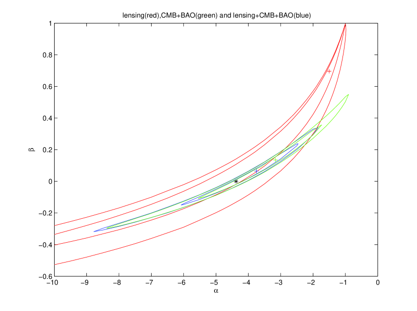
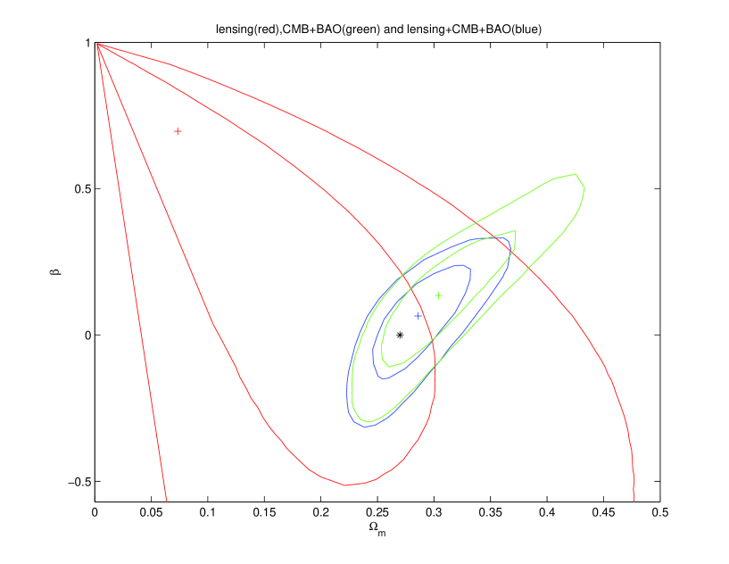
In the Friedmann equation [12], we can find the Ricci scalar R is always divided by , so we can choose units so that . For given , we can get the Ricci scalar today using the Friedmann equation. Then we can get through Eq. [10]. Now, we can get the relation between the Ricci scalar and the redshift through Eq. [10]. We use the 73 data to constrain f(R) gravity in Palatini approach. Fist, we show the parameter space in Figure 1. We can see the data is compatible with the H(z) data hz . The best-fit values are . Using the data only cannot give a stringent constraint. After adding the CMB and the BAO data, the parameters are tightly constrained. The best-fit values are . What we want to emphasis is the Hubble parameter should always be positive, which restricts the parameters further. We also exhibit the parameter space in Figure 2. The best-fit values are for data and for combination with CMB and BAO. Moreover, if we further fix , the best-fit value for is = for lensing data and = for combined data respectively. From the results above, we can see the CDM model which is corresponding to or is within range. In order to compare the data, we list some constraint results from other cosmological observations in Table 1.
| Test | Ref. | ||
|---|---|---|---|
| SNe Ia (SNLS) | constraintb | -12.5 | -0.6 |
| SNe Ia (SNLS) + BAO + CMB | constraintb | -4.63 | -0.027 |
| SNe Ia (Gold) | constrainta | -10 | -0.51 |
| SNe Ia (Gold) + BAO + CMB | constrainta | -3.6 | 0.09 |
| BAO | constrainta | -1.1 | 0.57 |
| CMB | constrainta | -8.4 | -0.27 |
| SNe Ia (Union) | constraintd | - | -0.99 |
| SNe Ia (Union) + BAO + CMB | constraintd | -3.45 | 0.12 |
| LSS | constraintc | - | -2.6 |
| H(z) | hz | -1.11 | 0.9 |
| H(z) + BAO + CMB | hz | -4.7 | -0.03 |
| Lensing() | This Letter | ||
| BAO+CMB | This Letter | ||
| Lensing() + BAO + CMB | This Letter |
5 Conclusion
In this Letter, we use data from lensing systems to constrain f(R) gravity in Palatini approach . Compared with references, we can see the constraint effects that data give can be compatible with other data (SNe Ia, H(z), BAO, CMB and so on). Moreover, we find although the best-fit values of the parameters are different from various observations, the directions of the contours in space are very similar, thus needing different observations to break the degeneracy. The data propose a new way to probe the cosmology dlds . As we expect, the lensing data alone cannot give a stringent constraint. There are at least three aspects that contribute to the error. First, the assumption that the lens galaxies satisfy SIS or SIE model may have some issues especially for four images. Second, the measurements of velocity dispersions have some uncertainties. Finally, the error exists due to the influence of line of sight mass contamination sight . Combining with CMB and BAO, it gives , which contains the CDM model. Until now, we cannot distinguish it from the standard cosmology, where . For future lensing study, in order to improve the constraint, we hope large survey projects can find more strong lensing systems. At the same time, a better understand about the lens model and more precise measurements can give us more stringent results and more information about f(R) gravity.
Acknowledgments This work was supported by the National Natural Science Foundation of China under the Distinguished Young Scholar Grant 10825313, the Ministry of Science and Technology national basic science Program (Project 973) under Grant No.2012CB821804, the Fundamental Research Funds for the Central Universities and Scientific Research Foundation of Beijing Normal University.
References
- (1) A. G. Riess, et al., ApJ, 501 (1998) 61; S. Perlmutter, et al., ApJ, 517 (1999) 565; A. C. Pope, et al., ApJ, 607 (2004) 655.
- (2) A. Cohen, D. Kaplan and A. Nelson, PRL, 82 (1999) 4971; M. Li, PLB, 603 (2004) 1.
- (3) P. J. E. Peebles and B. Ratra, ApJL, 325 (1988a) 17; P. J. E. Peebles and B. Ratra, PRD, 37 (1988b) 3406.
- (4) Z. K. Guo, Y. S. Piao and Y. Z. Zhang, PLB, 608 (2005) 177; B. Feng, X. wang and X. Zhang, PLB, 607 (2005) 35.
- (5) R. Caldwell, PLB, 545 (2002) 23.
- (6) M. C. Bento, O. Bertolami and A. A. Sen, PRD, 66 (2002) 043507; M. C. Bento, O. Bertolami and A. A. Sen, PRD, 70 (2002) 083519;
- (7) L. Randall and R. Sundrum, PRL, 83 (1999) 3370; J. S. Alcaniz, PRD, 65 (2002) 123514; C. Deffayet, et al., PRD, 65 (2002) 044023; V. Sahni and Y. Shtanov, JCAP, 0311 (2003) 014
- (8) R. Kerner, Gen. Rel. Gra., 14 (1982) 453; J. D. Barrow and S. Cotsakis, PLB, 214 (1988) 515; S. M. Carroll, et al., PRD, 70 (2004) 043528; S. Capozziello, et al., PRD, 71 (2005) 043503; S. Nojiri and S. D. Odintsov, Gen. Rel. Gra., 36 (2004) 1765.
- (9) S. Capozziello and M. Francaviglia, Gen. Rel. Gra., 40 (2008) 357; T. P. Sotiriou and V. Faraoni, Rev. Mod. Phys., 82 (2008)451.
- (10) T. P. Sotiriou, PRD, 73 (2006) 063515.
- (11) M. Amarzguioui, et al., A&A, 454 (2006) 707.
- (12) S. Fay, et al., PRD, 75 (2007) 063509.
- (13) T. Koivisto, PRD, 76 (2007) 043527.
- (14) J. Santos, et al., PLB, 669 (2008) 14.
- (15) T. P. Sotiriou, Gen. Rel. Gra., 23 (2006) 1253; A. Browne, et al., PRD, 74 (2006) 043502; X. J. Yang and D. M. Chen, MNRAS, 394 (2009) 1449.
- (16) T. Koivisto, PRD, 73 (2006) 083517.
- (17) B. Li and J. D. Barrow, PRD, 75 (2007) 084010.
- (18) K.-H. Chae, MNRAS, 346 (2003) 746; K.-H. Chae, et al., ApJ, 607 (2004) L71; Z.-H. Zhu, et al., A&A, 483 (2008) 15.
- (19) Z.-H. Zhu and X.-P. Wu, A&A, 324 (1997) 483; E. O. Ofek, et al., MNRAS, 343 (2003) 639.
- (20) T. Treu, et al., ApJ, 640 (2006) 662; M. Biesiada, et al., MNRAS, 406 (2010) 1055; E. Newton, et al., accepted by ApJ, 2011, arXiv:1104.2608; L. V. E. Koopmans and T. Treu, ApJ, 568 (2002) L5; L. V. E. Koopmans and T. Treu, ApJ, 583 (2003) 606; T. Treu and L. V. E. Koopmans, ApJ, 611 (2004) 739.
- (21) H. Yu and Z.-H. Zhu, submitted to RAA, arXiv:1011.6060; N. Ota and K. Mitsuda, A&A, 428 (2004) 757; Bonamente et al., ApJ, 647 (2006) 25; G. Covone, et al., submitted to A&A, 2005, arXiv:0511332; J. Richard, et al., ApJ, 662 (2007) 781.
- (22) J. R. Bond, et al., MNRAS, 291 (1997) L33.
- (23) E. Komatsu, et al., ApJS, 192 (2011) 18.
- (24) D. J. Eisenstein, et al., ApJ, 633 (2005) 560.
- (25) F. C. Carvalho, et al., JCAP, 0809 (2008) 008
- (26) S. Cao and Z.-H Zhu, 2011, arXiv:1105.6226, accepted by JCAP.
- (27) M. Biesiada, A. Piorkowska and B. Makec, MNRAS, 406 (2010) 1055.
- (28) N. Dalal, et al., ApJ, 622 (2005) 99; I. Momcheva, et al., ApJ, 641 (2006) 169.
| Cluster/galaxy | zs | zl | ||
|---|---|---|---|---|
| MS 0451.6-0305 | 2.91 | 0.550 | 0.785 | 0.087 |
| 3C220.1 | 1.49 | 0.61 | 0.611 | 0.530 |
| CL0024.0 | 1.675 | 0.391 | 0.919 | 0.430 |
| Abell 2390 | 4.05 | 0.228 | 0.737 | 0.053 |
| Abell 2667 | 1.034 | 0.226 | 0.837 | 0.124 |
| Abell 68 | 1.6 | 0.255 | 0.982 | 0.225 |
| MS 1512.4 | 2.72 | 0.372 | 0.734 | 0.330 |
| MS 2137.3-2353 | 1.501 | 0.313 | 0.778 | 0.105 |
| MS 2053.7 | 3.146 | 0.583 | 0.968 | 0.209 |
| PKS 0745-191 | 0.433 | 0.103 | 0.818 | 0.065 |
| SDSS J0037-0942 | 0.6322 | 0.1955 | 0.6418 | 0.0501 |
| SDSS J0216-0813 | 0.5235 | 0.3317 | 0.3278 | 0.0451 |
| SDSS J0737+3216 | 0.5812 | 0.3223 | 0.3365 | 0.033 |
| SDSS J0912+0029 | 0.324 | 0.1642 | 0.5293 | 0.0391 |
| SDSS J0956+5100 | 0.47 | 0.2405 | 0.4532 | 0.0485 |
| SDSS J0959+0410 | 0.5349 | 0.126 | 0.6621 | 0.0752 |
| SDSS J1250+0523 | 0.795 | 0.2318 | 0.5319 | 0.0582 |
| SDSS J1330-0148 | 0.7115 | 0.0808 | 0.7762 | 0.0796 |
| SDSS J1402+6321 | 0.4814 | 0.2046 | 0.5739 | 0.0633 |
| SDSS J1420+6019 | 0.5352 | 0.0629 | 0.851 | 0.0413 |
| SDSS J1627-0053 | 0.5241 | 0.2076 | 0.4828 | 0.0426 |
| SDSS J1630+4520 | 0.7933 | 0.2479 | 0.8074 | 0.0984 |
| SDSS J2300+0022 | 0.4635 | 0.2285 | 0.4666 | 0.0581 |
| SDSS J2303+1422 | 0.517 | 0.1553 | 0.7754 | 0.0916 |
| SDSS J2321-0939 | 0.5324 | 0.0819 | 0.9082 | 0.0519 |
| Q0047-2808 | 3.595 | 0.485 | 0.8872 | 0.1162 |
| CFRS03-1077 | 2.941 | 0.938 | 0.6834 | 0.1035 |
| HST 14176 | 3.399 | 0.81 | 0.9757 | 0.1307 |
| HST 15433 | 2.092 | 0.497 | 0.929 | 0.1602 |
| MG 2016 | 3.263 | 1.004 | 0.5035 | 0.0982 |
| SDSS J0029-0055 | 0.9313 | 0.227 | 0.6356 | 0.0999 |
| SDSS J0044+0113 | 0.1965 | 0.1196 | 0.3877 | 0.0379 |
| SDSS J0109+1500 | 0.5248 | 0.2939 | 0.3803 | 0.0576 |
| SDSS J0330-0020 | 1.0709 | 0.3507 | 0.8498 | 0.1684 |
| SDSS J0728+3835 | 0.6877 | 0.2058 | 0.9477 | 0.0974 |
| SDSS J0822+2652 | 0.5941 | 0.2414 | 0.6056 | 0.0701 |
| SDSS J0841+3824 | 0.6567 | 0.1159 | 0.9671 | 0.0946 |
| SDSS J0935-0003 | 0.467 | 0.3475 | 0.1926 | 0.0341 |
| SDSS J0936+0913 | 0.588 | 0.1897 | 0.6409 | 0.0633 |
| SDSS J0946+1006 | 0.6085 | 0.2219 | 0.6927 | 0.1106 |
| SDSS J0955+0101 | 0.3159 | 0.1109 | 0.8571 | 0.1161 |
| SDSS J0959+4416 | 0.5315 | 0.2369 | 0.5599 | 0.0872 |
| SDSS J1016+3859 | 0.4394 | 0.1679 | 0.6204 | 0.0653 |
| SDSS J1020+1122 | 0.553 | 0.2822 | 0.524 | 0.0669 |
| SDSS J1023+4230 | 0.696 | 0.1912 | 0.836 | 0.1036 |
| SDSS J1029+0420 | 0.6154 | 0.1045 | 0.7952 | 0.0833 |
| SDSS J1032+5322 | 0.329 | 0.1334 | 0.4082 | 0.0414 |
| SDSS J1103+5322 | 0.7353 | 0.1582 | 0.9219 | 0.1129 |
| SDSS J1106+5228 | 0.4069 | 0.0955 | 0.6222 | 0.0617 |
| SDSS J1112+0826 | 0.6295 | 0.273 | 0.5052 | 0.0632 |
| SDSS J1134+6027 | 0.4742 | 0.1528 | 0.6687 | 0.0671 |
| SDSS J1142+1001 | 0.5039 | 0.2218 | 0.6967 | 0.1387 |
| SDSS J1143-0144 | 0.4019 | 0.106 | 0.8061 | 0.0779 |
| SDSS J1153+4612 | 0.8751 | 0.1797 | 0.7138 | 0.0948 |
| SDSS J1204+0358 | 0.6307 | 0.1644 | 0.6381 | 0.0813 |
| SDSS J1205+4910 | 0.4808 | 0.215 | 0.5365 | 0.0535 |
| SDSS J1213+6708 | 0.6402 | 0.1229 | 0.5783 | 0.0594 |
| SDSS J1403+0006 | 0.473 | 0.1888 | 0.6352 | 0.1014 |
| SDSS J1416+5136 | 0.8111 | 0.2987 | 0.8259 | 0.1721 |
| SDSS J1430+4105 | 0.5753 | 0.285 | 0.509 | 0.1012 |
| SDSS J1436-0000 | 0.8049 | 0.2852 | 0.775 | 0.1176 |
| SDSS J1443+0304 | 0.4187 | 0.1338 | 0.6439 | 0.0678 |
| SDSS J1451-0239 | 0.5203 | 0.1254 | 0.7262 | 0.0912 |
| SDSS J1525+3327 | 0.7173 | 0.3583 | 0.6526 | 0.1285 |
| SDSS J1531-0105 | 0.7439 | 0.1596 | 0.7628 | 0.0766 |
| SDSS J1538+5817 | 0.5312 | 0.1428 | 0.972 | 0.1234 |
| SDSS J1621+3931 | 0.6021 | 0.2449 | 0.8042 | 0.1363 |
| SDSS J1636+4707 | 0.6745 | 0.2282 | 0.7093 | 0.0921 |
| PG1115+080 | 1.72 | 0.31 | 0.7036 | 0.1252 |
| MG1549+3047 | 1.17 | 0.11 | 0.5728 | 0.0908 |
| Q2237+030 | 1.169 | 0.04 | 0.6685 | 0.1866 |
| CY2201-3201 | 3.9 | 0.32 | 0.8526 | 0.2624 |
| B1608+656 | 1.39 | 0.63 | 0.646 | 0.1831 |