Gravitational waves and the breaking of parallelograms in space-time

We show that plane-fronted gravitational waves induce the breaking of parallelograms in space-time, in the context of the teleparallel equivalent of general relativity (TEGR). The breaking of parallelograms can be shown by considering a thought experiment that consists of a simple physical configuration, similar to the experimental setup that is expected to lead to the measurement of gravitational waves with the use of laser interferometers. An incident beam of light splits into two beams running along perpendicular arms, endowed with fixed mirrors at the extremes. The reflected light beams are detected at the same point of the splitting. Along each arm, the two light beams define two null vectors: the forward vector and the reflected vector. We show that the sum of these four vectors, the forward and reflected null vectors along the two arms, do form a parallelogram in flat space-time, but not in the presence of plane-fronted gravitational waves. The non-closure of the parallelogram is a manifestation of the torsion of the space-time, and in this context indicates the existence of gravitational waves.

PACS numbers: 04.20.-q, 04.20.Cv, 04.30.-w

(a) wadih@unb.br, jwmaluf@gmail.com

(b) sc.ulhoa@gmail.com

(c) rocha@fis.unb.br

1 Introduction

The dynamics of the gravitational field may be described either in terms of the metric and curvature tensors, or in terms of the tetrad fields and the torsion tensor. The latter approach is known as teleparallel gravity. The reformulation of Einstein’s theory in terms of tetrad fields and of the torsion tensor is the teleparallel equivalent of general relativity (TEGR) [1, 2, 3, 4, 5]. The field equations for the gravitational field in the standard metric formulation and in the TEGR are essentially the same. However, different geometrical frameworks naturally lead to different approaches and forms of investigation of the theory. In particular, in the TEGR there are definitions and physical results that are expressed in terms of the torsion tensor.

Gravitational waves are one of the most important consequences of general relativity. They are due to the dynamical nature of space-time, which we consider to be described by Einstein’s equations. It is natural to consider a gravitational wave as a kind of ripple in the background flat geometry. Gravitational waves may be classified either as non-linear waves, which are exact solutions of Einstein’s equations, or linearized waves, which are solutions of the linearized Einstein’s equations, presented in standard textbooks on general relativity. One of the simplest realizations of a non-linear gravitational wave is given by the solution known as plane-fronted gravitational wave, studied by Ehlers and Kundt [6].

The present attempts to observe gravitational waves are based on laser interferometers, constituted by two long and perpendicular arms that are able, in principle, to detect gravitational waves travelling in the direction normal the plane formed by the two arms (see, for instance, Refs. [7, 8]). The mirrors at the end of the long arms may be attached to test masses that are hung from wires, and are free to swing in the horizontal directions, or may be fixed at the end of the arms. In the present setup, the mirrors are fixed at the end of the arms.

In this article, we will consider a thought experiment that consists in laser beams travelling back and forth along perpendicular arms, in the presence of a plane-fronted gravitational wave travelling in the $z$ direction. Let us denote by $v^{\mu}$ and $w^{\mu}$ the null vectors that represent, respectively, (i) the laser beam trajectory from the splitting point $S$ to the fixed mirror $M_{1}$, and (ii) from $M_{1}$ back to $S$, along the $x$ direction. Along the $y$ direction, the vectors $a^{\mu}$ and $b^{\mu}$ travel (iii) from the splitting point $S$ to the fixed mirror $M_{2}$, and (iv) from $M_{2}$ back to $S$, respectively. In flat space-time, these four null vectors form a parallelogram in the sense that $v^{\mu}+w^{\mu}=a^{\mu}+b^{\mu}$. We will show in this analysis that in the presence of a plane-fronted gravitational wave, these null vectors no longer form a parallelogram, because $v^{\mu}+w^{\mu}\neq a^{\mu}+b^{\mu}$. This fact is an indication that the space-time has torsion. By establishing the tetrad frame adapted to stationary observers in the space-time of plane-fronted gravitational waves, we will obtain the torsion tensor that precisely explains the breaking of the parallelogram. The result described here is geometrically similar to the breaking of parallelograms in the Schwarzschild space-time, in the context of the Pound-Rebka experiment [9, 10]. The breaking of parallelograms shows that torsion is an intrinsic geometric property of space-time, and indicates the presence of gravitational waves. In the present approach, the existence of gravitational waves is verified by the lapse of time between the arrival of the two reflected (perpendicular) light beams, as we will see.

The article is organized as follows. In Section 2 we recall the interpretation of tetrad fields as frames adapted to arbitrary observers in space-time. In Section 3 the TEGR is briefly presented. The breaking of parallelograms in the space-time of plane-fronted gravitational waves is discussed in Sections 4 and 5. In Section 6 we present our conclusions.

Notation: space-time indices $\mu,\nu,...$ and SO(3,1) indices $a,b,...$ run from 0 to 3. Time and space indices are indicated according to $\mu=0,i,\;\;a=(0),(i)$. The tetrad fields are denoted $e^{a}\,_{\mu}$, and the torsion tensor reads $T_{a\mu\nu}=\partial_{\mu}e_{a\nu}-\partial_{\nu}e_{a\mu}$. The flat, Minkowski space-time metric tensor raises and lowers tetrad indices and is fixed by $\eta_{ab}=e_{a\mu}e_{b\nu}g^{\mu\nu}=diag(-1,1,1,1)$. The determinant of the tetrad fields is represented by $e=\det(e^{a}\,_{\mu})$.

The torsion tensor defined above is often related to the object of anholonomity $\Omega^{\lambda}\,_{\mu\nu}$ via $\Omega^{\lambda}\,_{\mu\nu}=e_{a}\,^{\lambda}T^{a}\,_{\mu\nu}$. However, we assume that the space-time geometry is defined by the tetrad fields only, and in this case the only possible non-trivial definition for the torsion tensor is given by $T^{a}\,_{\mu\nu}$. This torsion tensor is related to the antisymmetric part of the Weitzenböck connection $\Gamma^{\lambda}_{\mu\nu}=e^{a\lambda}\partial_{\mu}e_{a\nu}$, which establishes the Weitzenböck space-time. The curvature of the Weitzenböck connection vanishes. However, the tetrad fields also yield the metric tensor, which establishes the Riemannian geometry. Therefore in the framework of a geometrical theory based only on tetrad fields, one may use the concepts of both Riemannian and Weitzenböck geometries.

2 Tetrad fields as reference frames

We recall the discussion presented in Refs. [11, 12] regarding the characterization of tetrad fields as reference frames in space-time. A frame may be characterized in a coordinate invariant way by the inertial accelerations, represented by the acceleration tensor.

We denote by $x^{\mu}(s)$ the worldline $C$ of an observer in space-time, where $s$ is the proper time of the observer. The velocity of the observer on $C$ reads $u^{\mu}=dx^{\mu}/ds$. The observer’s velocity is identified with the $a=(0)$ component of $e_{a}\,^{\mu}$: $u^{\mu}(s)=e_{(0)}\,^{\mu}$ (we are assuming $c=1$ for the speed of light). The acceleration $a^{\mu}$ of the observer is given by the absolute derivative of $u^{\mu}$ along $C$ [13],

$$a^{\mu}={{Du^{\mu}}\over{ds}}={{De_{(0)}\,^{\mu}}\over{ds}}=u^{\alpha}\nabla_{\alpha}e_{(0)}\,^{\mu}\,,$$ (1)

where the covariant derivative is constructed out of the Christoffel symbols. Thus, $e_{a}\,^{\mu}$ and its derivatives determine the velocity and acceleration of an observer along the worldline. The set of tetrad fields for which $e_{(0)}\,^{\mu}$ describe a congruence of timelike curves is adapted to a class of observers characterized by the velocity field $u^{\mu}=e_{(0)}\,^{\mu}$ and by the acceleration $a^{\mu}$.

We may consider not only the acceleration of observers along trajectories whose tangent vectors are given by $e_{(0)}\,^{\mu}$, but the acceleration of the whole frame along $C$. The acceleration of the frame is determined by the absolute derivative of $e_{a}\,^{\mu}$ along the path $x^{\mu}(s)$. Thus, assuming that the observer carries an orthonormal tetrad frame $e_{a}\,^{\mu}$, the acceleration of the latter along the path is given by [14]

$${{De_{a}\,^{\mu}}\over{ds}}=\phi_{a}\,^{b}\,e_{b}\,^{\mu}\,,$$ (2)

where $\phi_{ab}$ is the antisymmetric acceleration tensor. According to Ref. [14], in analogy with the Faraday tensor we may identify $\phi_{ab}\rightarrow({\bf a},{\bf\Omega})$, where ${\bf a}$ is the translational acceleration ($\phi_{(0)(i)}=a_{(i)}$) and ${\bf\Omega}$ is the angular velocity of the local spatial frame with respect to a non-rotating (Fermi-Walker transported) frame. It follows that

$$\phi_{a}\,^{b}=e^{b}\,_{\mu}{{De_{a}\,^{\mu}}\over{ds}}=e^{b}\,_{\mu}\,u^{\lambda}\nabla_{\lambda}e_{a}\,^{\mu}\,.$$ (3)

Therefore, given any set of tetrad fields for an arbitrary gravitational field configuration, its geometrical interpretation may be obtained by interpreting $e_{(0)}\,^{\mu}=u^{\mu}$, where $u^{\mu}$ is the velocity of the observer, and by the values of the acceleration tensor $\phi_{ab}$.

The acceleration vector $a^{\mu}$ defined by Eq. (1) may be projected on a frame in order to yield

$$a^{b}=e^{b}\,_{\mu}a^{\mu}=e^{b}\,_{\mu}u^{\alpha}\nabla_{\alpha}e_{(0)}\,^{\mu}=\phi_{(0)}\,^{b}\,.$$ (4)

Thus, $a^{\mu}$ and $\phi_{(0)(i)}$ are not different accelerations of the frame. The acceleration $a^{\mu}$ may be rewritten as

$$a^{\mu} = u^{\alpha}\nabla_{\alpha}e_{(0)}\,^{\mu}=u^{\alpha}\nabla_{\alpha}u^{\mu}={{dx^{\alpha}}\over{ds}}\biggl{(}{{\partial u^{\mu}}\over{\partial x^{\alpha}}}+\,^{0}\Gamma^{\mu}_{\alpha\beta}u^{\beta}\biggr{)}$$ (5)

$$= {{d^{2}x^{\mu}}\over{ds^{2}}}+\,^{0}\Gamma^{\mu}_{\alpha\beta}{{dx^{\alpha}}\over{ds}}{{dx^{\beta}}\over{ds}}\,,$$

where ${}^{0}\Gamma^{\mu}_{\alpha\beta}$ are the Christoffel symbols. If $u^{\mu}=e_{(0)}\,^{\mu}$ represents a geodesic trajectory, then the frame is in free fall and $a^{\mu}=0=\phi_{(0)(i)}$. Therefore we conclude that nonvanishing values of $\phi_{(0)(i)}$ represent inertial accelerations of the frame.

Following Ref. [11], we take into account the orthogonality of the tetrads and write Eq. (3) as $\phi_{a}\,^{b}=-u^{\lambda}e_{a}\,^{\mu}\nabla_{\lambda}e^{b}\,_{\mu}$, where $\nabla_{\lambda}e^{b}\,_{\mu}=\partial_{\lambda}e^{b}\,_{\mu}-\,^{0}\Gamma^{\sigma}_{\lambda\mu}e^{b}\,_{\sigma}$. Next we consider the identity $\partial_{\lambda}e^{b}\,_{\mu}-\,^{0}\Gamma^{\sigma}_{\lambda\mu}e^{b}\,_{\sigma}+\,\,^{0}\omega_{\lambda}\,^{b}\,{}_{c}e^{c}\,_{\mu}=0$, where ${}^{0}\omega_{\lambda}\,^{b}\,{}_{c}$ is the metric compatible Levi-Civita connection given by

$${}^{o}\omega_{\mu ab}=-{1\over 2}e^{c}\,_{\mu}(\Omega_{abc}-\Omega_{bac}-\Omega_{cab})\;,$$

$$\Omega_{abc}=e_{a\nu}(e_{b}\,^{\mu}\partial_{\mu}e_{c}\,^{\nu}-e_{c}\,^{\mu}\partial_{\mu}e_{b}\,^{\nu})\;,$$

and express $\phi_{a}\,^{b}$ according to

$$\phi_{a}\,^{b}=e_{(0)}\,^{\mu}(\,\,^{0}\omega_{\mu}\,^{b}\,{}_{a})\,.$$ (6)

Finally we take into account the identity $\,\,{}^{0}\omega_{\mu}\,^{a}\,{}_{b}=-K_{\mu}\,^{a}\,{}_{b}$, where $K_{\mu}\,^{a}\,{}_{b}$ is the contorsion tensor defined by

$$K_{\mu ab}={1\over 2}e_{a}\,^{\lambda}e_{b}\,^{\nu}(T_{\lambda\mu\nu}+T_{\nu\lambda\mu}+T_{\mu\lambda\nu})\,,$$ (7)

and $T_{\lambda\mu\nu}=e^{a}\,_{\lambda}T_{a\mu\nu}$. After simple manipulations we arrive at

$$\phi_{ab}={1\over 2}[T_{(0)ab}+T_{a(0)b}-T_{b(0)a}]\,.$$ (8)

The expression above is not invariant under local SO(3,1) transformations, and for this reason the values of $\phi_{ab}$ may characterize the frame. However, Eq. (8) is invariant under coordinate transformations. We interpret $\phi_{ab}$ as the inertial accelerations of the frame. An alternative (kinematic) characterization of the frame consists in (i) identifying, as above, the timelike component $e_{(0)}\,^{\mu}$ of the tetrad field with the velocity $u^{\mu}$ of the observer, i.e., $e_{(0)}\,^{\mu}=u^{\mu}$, and (ii) specifying the orientation of the spacelike components $e_{(i)}\,^{\mu}$ (along the standard unit vectors of orientation at spatial infinity, for instance). In both forms of characterization, six components of the tetrad field are fixed.

In Ref. [11] we applied definition (8) to the analysis of two simple configurations of tetrad fields in the flat Minkowski spacetime. We considered the frame adapted to linearly accelerated observers, and to a stationary frame whose four-velocity is $e_{(0)}\,^{\mu}=(1,0,0,0)$ and which rotates around the $z$ axis. The components $\phi_{(0)(i)}$ and $\phi_{(i)(j)}$ yield the known and expected values of the translational acceleration and of the angular velocity of the frame, respectively.

3 The teleparallel equivalent of general relativity

We are assuming that the space-time geometry is defined by the tetrad fields only. In this case the only possible definition for the torsion tensor is given by $T_{a\mu\nu}=\partial_{\mu}e_{a\nu}-\partial_{\nu}e_{a\mu}$. The equivalence of the TEGR with Einstein’s general relativity may be understood by means of an identity between the scalar curvature $R(e)$ constructed out of the tetrad fields, and a combination of quadratic terms of the torsion tensor,

$$eR(e)\equiv-e({1\over 4}T^{abc}T_{abc}+{1\over 2}T^{abc}T_{bac}-T^{a}T_{a})+2\partial_{\mu}(eT^{\mu})\,.$$ (9)

The formulation of Einstein’s general relativity in the context of the teleparallel geometry is discussed in Refs. [2, 3, 4, 5, 15]. The Lagrangian density of the TEGR is given by the combination of the quadratic terms on the right hand side of eq. (9),

$$L = -ke({1\over 4}T^{abc}T_{abc}+{1\over 2}T^{abc}T_{bac}-T^{a}T_{a})-L_{M}$$ (10)

$$\equiv -ke\Sigma^{abc}T_{abc}-L_{M}\,,$$

where $k=c^{3}/16\pi G$, $T_{a}=T^{b}\,_{ba}$, $T_{abc}=e_{b}\,^{\mu}e_{c}\,^{\nu}T_{a\mu\nu}$ and

$$\Sigma^{abc}={1\over 4}(T^{abc}+T^{bac}-T^{cab})+{1\over 2}(\eta^{ac}T^{b}-\eta^{ab}T^{c})\;.$$ (11)

$L_{M}$ stands for the Lagrangian density of the matter fields. The field equations derived from (10) are equivalent to Einstein’s equations. They read

$$e_{a\lambda}e_{b\mu}\partial_{\nu}(e\Sigma^{b\lambda\nu})-e(\Sigma^{b\nu}\,_{a}T_{b\nu\mu}-{1\over 4}e_{a\mu}T_{bcd}\Sigma^{bcd})={1\over{4k}}eT_{a\mu}\,,$$ (12)

where $\delta L_{M}/\delta e^{a\mu}=eT_{a\mu}$. It is possible to show that the left hand side of the equation above may be rewritten as ${1\over 2}e\left[R_{a\mu}(e)-{1\over 2}e_{a\mu}R(e)\right]$, which proves the equivalence of the present formulation with Einstein’s theory.

Equation (12) may be simplified as

$$\partial_{\nu}(e\Sigma^{a\lambda\nu})={1\over{4k}}e\,e^{a}\,_{\mu}(t^{\lambda\mu}+T^{\lambda\mu})\;,$$ (13)

where $T^{\lambda\mu}=e_{a}\,^{\lambda}T^{a\mu}$ and $t^{\lambda\mu}$ is defined by

$$t^{\lambda\mu}=k(4\Sigma^{bc\lambda}T_{bc}\,^{\mu}-g^{\lambda\mu}\Sigma^{bcd}T_{bcd})\,.$$ (14)

In view of the antisymmetry property $\Sigma^{a\mu\nu}=-\Sigma^{a\nu\mu}$ it follows that

$$\partial_{\lambda}\left[e\,e^{a}\,_{\mu}(t^{\lambda\mu}+T^{\lambda\mu})\right]=0\,.$$ (15)

The equation above yields the continuity (or balance) equation,

$${d\over{dt}}\int_{V}d^{3}x\,e\,e^{a}\,_{\mu}(t^{0\mu}+T^{0\mu})=-\oint_{S}dS_{j}\,\left[e\,e^{a}\,_{\mu}(t^{j\mu}+T^{j\mu})\right]\,.$$ (16)

We identify $t^{\lambda\mu}$ as the gravitational energy-momentum tensor [4], and

$$P^{a}=\int_{V}d^{3}x\,e\,e^{a}\,_{\mu}(t^{0\mu}+T^{0\mu})\,,$$ (17)

as the total energy-momentum contained within a volume $V$ of the three-dimensional space. In view of (13), Eq. (17) may be written as

$$P^{a}=-\int_{V}d^{3}x\partial_{j}\Pi^{aj}\,,$$ (18)

where $\Pi^{aj}=-4ke\,\Sigma^{a0j}$, which is the momentum canonically conjugated to $e_{aj}$ [3, 4]. The expression above is the definition for the gravitational energy-momentum discussed in Refs. [17, 4], obtained in the framework of the Hamiltonian vacuum field equations. We note that (15) is a true energy-momentum conservation equation.

The emergence of a nontrivial total divergence is a feature of theories with torsion. The integration of this total divergence yields a surface integral. If we consider the $a=(0)$ component of Eq. (18) and adopt asymptotic boundary conditions for the tetrad fields, we find [17] that the resulting expression is precisely the surface integral at infinity that defines the ADM energy [16]. This fact is a strong indication that Eq. (10) does indeed represent the gravitational energy-momentum.

4 The breaking of parallelograms in space-time

We will consider the space-time of a plane-fronted gravitational wave. The space-time is described by a line element that is an exact solution of Einstein’s equations, and is given by [6, 18]

$$ds^{2}=dx^{2}+dy^{2}+2du\,dv+H(x,y,u)du^{2}\,.$$ (19)

As in Section 2, we assume $c=1$. The function $H(x,y,u)$ satisfies

$$\biggl{(}{\partial^{2}\over{\partial x^{2}}}+{\partial^{2}\over{\partial y^{2}}}\biggr{)}H(x,y,u)=0\,.$$ (20)

Transforming the $(u,v)$ to $(t,z)$ coordinates, where

$$u={1\over\sqrt{2}}(z-t)\,,\ \ \ \ v={1\over\sqrt{2}}(z+t)\,,$$

we find

$$ds^{2}=\biggl{(}{H\over 2}-1\biggr{)}dt^{2}+dx^{2}+dy^{2}+\biggl{(}{H\over 2}+1\biggr{)}dz^{2}-H\,dtdz\,.$$ (21)

The function $H$ is required to satisfy only Eq. (20). However, it would be interesting to specify $H$ such that it describes a wave-packet [18].

Before we investigate the action of a plane-fronted gravitational wave in the experimental setup, let us establish the physical configuration first in flat space-time, according to the discussion in Section 1. We will consider a laser beam in the $xy$ plane that splits into two beams: one beam along an arm of proper length $L$, in the $x$ direction, and another beam along a similar arm, also with length $L$, in the $y$ direction. The splitting point is denoted by $S$, and has coordinates $(x_{0},y_{0})$. At the ends of each arm there are fixed mirrors, $M_{1}$ and $M_{2}$, that reflect the light beams back to the splitting point $S$. The experimental setup is displayed in Fig. 1. It may be characterized as a parallelogram in the $(+x,+y)$ directions. In Section 5 we will also consider the $(+x,-x)$ and $(+x,-y)$ directions.

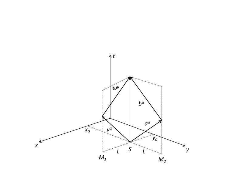
Figure 1: The parallelogram in the $(+x,+y)$ directions

The trajectory of a light ray in the $x$ direction is described by a null vector $v^{\mu}(t,x,y,z)=(v^{0},v^{1},0,0)$ that satisfies the condition $v^{\mu}v^{\nu}g_{\mu\nu}=0$. For a light ray travelling in the positive direction along the $x$ axis, the latter condition yields $v^{1}=(-g_{00}/g_{11})^{1/2}\,v_{0}=(1-H/2)^{1/2}\,v_{0}$. We will fix the value of $v^{1}$ by means of the following procedure. For a vector $v^{\mu}$ that represents a light ray between the point $S$ and the position $M_{1}$ of the mirror, we require $v^{1}$ to have length $L$, in the presence of a plane fronted gravitational wave. Thus we require

$$v^{1}=\int_{x_{0}}^{x_{0}+L}dx\,\sqrt{g_{11}}=L\,.$$ (22)

It follows that

$$v^{0}={L\over{(1-H/2)^{1/2}}}\,,\ \ \ \ \ H=H(x^{0}+L,y_{0},t_{0}+dt)\,,$$ (23)

where $t_{0}$ is the time coordinate of the emitted light ray at the point $S$, and $t_{0}+dt$ is the time coordinate when the light ray reaches $M_{1}$. In flat space-time, the reflected light ray returns to the point $S$ in the time coordinate $t_{0}+2dt$. The values $t_{0}$, $t_{0}+dt$ and $t_{0}+2dt$ parametrize the physical events also in the presence of a plane-fronted gravitational wave. Therefore the vector $v^{\mu}$ is defined by

$$v^{\mu}=\biggl{(}{L\over{(1-H/2)^{1/2}}},L,0,0\biggl{)}\,,\ \ \ \ \ H=H(x_{0}+L,y_{0},t_{0}+dt)\,.$$ (24)

We define the reflected vector $w^{\mu}$, that travels from $M_{1}$ back to $S$, according to

$$w^{\mu}=\biggl{(}{L\over{(1-H/2)^{1/2}}},-L,0,0\biggl{)}\,,\ \ \ \ \ H=H(x_{0},y_{0},t_{0}+2dt)\,.$$ (25)

Expression (22) for the component $v_{1}$ holds only for a plane-fronted gravitational wave. Note that in the context of a linearized wave, $v_{1}$ would not be given by Eq. (22); it would be time dependent.

Along the $y$ direction, the vectors $a^{\mu}$ and $b^{\mu}$ that travel from $S$ to the mirror $M_{2}$, and from $M_{2}$ back to $S$, are constructed in similarity to $v^{\mu}$ and $w^{\mu}$. They read

$$a^{\mu}=\biggl{(}{L\over{(1-H/2)^{1/2}}},0,L,0\biggl{)}\,,\ \ \ \ \ H=H(x_{0},y_{0}+L,t_{0}+dt)\,,$$ (26)

$$b^{\mu}=\biggl{(}{L\over{(1-H/2)^{1/2}}},0,-L,0\biggl{)}\,,\ \ \ \ \ H=H(x_{0},y_{0},t_{0}+2dt)\,.$$ (27)

The vectors $v^{\mu}$, $w^{\mu}$, $a^{\mu}$ and $b^{\mu}$ are defined for a fixed coordinate position $z_{0}$. They are located at $(x_{0}+L,y_{0},t_{0}+dt)$, $(x_{0},y_{0},t_{0}+2dt)$, $(x_{0},y_{0}+L,t_{0}+dt)$ and $(x_{0},y_{0},t_{0}+2dt)$, respectively. We find it suitable to depict them as in Fig. 1, since they do form a parallelogram in a flat geometry.

Let us define the breaking of the parallelogram in space-time by the vector

$$\Delta^{\mu}=(v^{\mu}+w^{\mu})-(a^{\mu}+b^{\mu})\,.$$ (28)

It is easy to see that for $i=1,2,3$ we have $\Delta^{i}=0$, and that for $\Delta^{0}$ we have

$$\Delta^{0} = L\biggl{\{}{1\over{[1-{1\over 2}H(x_{0}+L,y_{0},t_{0}+dt)]^{1/2}}}$$ (29)

$$+{1\over{[1-{1\over 2}H(x_{0},y_{0},t_{0}+2dt)]^{1/2}}}$$

$$-{1\over{[1-{1\over 2}H(x_{0},y_{0}+L,t_{0}+dt)]^{1/2}}}$$

$$-{1\over{[1-{1\over 2}H(x_{0},y_{0},t_{0}+2dt)]^{1/2}}}\biggl{\}}\,.$$

The second and fourth terms above cancel each other, and we are left with

$$\Delta^{0}=L{\{[1-{1\over 2}H(x_{0},y_{0}+L,t_{0}+dt)]^{1/2}-[1-{1\over 2}H(x_{0}+L,y_{0},t_{0}+dt)]^{1/2}\}\over[1-{1\over 2}H(x_{0}+L,y_{0},t_{0}+dt)]^{1/2}[1-{1\over 2}H(x_{0},y_{0}+L,t_{0}+dt)]^{1/2}}\,.$$ (30)

The only assumption we make in this analysis is that $L$ is sufficiently small, so that we can expand $H$ in terms of $L$ according to

$$H(x_{0}+L,y_{0},t_{0})\approx H(x_{0},y_{0},t_{0})+{{\partial H(x_{0},y_{0},t_{0})}\over{\partial x}}L\equiv H+{{\partial H}\over{\partial x}}L\,.$$ (31)

Likewise,

$$H(x_{0},y_{0}+L,t_{0})\approx H(x_{0},y_{0},t_{0})+{{\partial H(x_{0},y_{0},t_{0})}\over{\partial y}}L\equiv H+{{\partial H}\over{\partial y}}L\,.$$ (32)

We may consider the function $H$ to represent a wave packet in the form of a Gaussian function, that travels in the $z$ direction. The approximation above holds if $L$ is much smaller compared to the width of the Gaussian (or if $H$ varies very weakly over the space region of Fig. 1). In view of the approximation above, Eq. (30) is finally simplified to

$$\Delta^{0}={L^{2}\over 4}\biggl{[}{{({{\partial H}\over{\partial x}})-({{\partial H}\over{\partial y}})}\over{(1-{1\over 2}H)^{3/2}}}\biggr{]}\,.$$ (33)

The equation above expresses the non-closure in space-time of the parallelogram displayed in Fig. 1, and thus indicates the presence of torsion in the space-time geometry.

We will present here the torsion tensor that precisely explains the breaking of the parallelogram of Fig. 1. For this purpose, we need to establish the reference frame for the measurement of $\Delta^{0}$. This reference frame is the same one adopted in Ref. [19], in the analysis of the energy-momentum of plane-fronted gravitational waves. As in Section 2, we denote by $x^{\mu}(s)$ the worldline $C$ of an arbitrary observer in space-time, and by $u^{\mu}=dx^{\mu}/ds$ its velocity along $C$. We identify the timelike component $e_{(0)}\,^{\mu}$ of the inverse tetrad field with the velocity of the observer, i.e., $e_{(0)}\,^{\mu}=u^{\mu}$. The components $e_{(i)}\,^{\mu}$, for $i=1,2,3$ may be specified by requiring these spacelike vectors to be oriented asymptotically along the three Cartesian axes $x,y,z$. The tetrad frame established in Ref. [19] is well suited for our purposes.

We will consider the stationary observer determined by the worldline of the splitting point $S$, which is characterized by the condition $e_{(0)}\,^{i}=0$. A suitable construction of a tetrad frame, adapted to the stationary character of the observer, is [19]

$$e_{a\mu}=\pmatrix{-A&0&0&-B\cr 0&1&0&0\cr 0&0&1&0\cr 0&0&0&C}\,,$$ (34)

where

$$A=\biggl{(}1-{H\over 2}\biggr{)}^{1/2}\,,\ \ \ \ AB={H\over 2}\,,\ \ \ \ \ AC=1\,.$$ (35)

In (34), $a$ and $\mu$ label rows and columns, respectively. It is not difficult to verify that Eq. (34) yields [19]

$$e_{(0)}\,^{\mu}=(1/A,0,0,0)\,,$$ (36)

and

$$e_{(1)}\,^{\mu} = (0,1,0,0)\,,$$

$$e_{(2)}\,^{\mu} = (0,0,1,0)\,,$$

$$e_{(3)}\,^{\mu} = (\,-H/(2A)\,,0,0,A).$$ (37)

Note that if $H\ll 1$ we have $A\cong 1-H/4$ and therefore $e_{(3)}\,^{i}=(0,0,A)\cong(0,0,1-H/4)$.

The frame is determined by fixing six conditions on $e_{a\mu}$. Equation (36) fixes the kinematic state of the frame, since the three velocity conditions $e_{(0)}\,^{i}=0$ ensure that the frame is stationary. Three other conditions fix the spatial orientation of the frame. According to Eq. (37), $e_{(1)}\,^{\mu}$, $e_{(2)}\,^{\mu}$ and $e_{(3)}\,^{\mu}$ are unit vectors along the $x$, $y$ and $z$ axis, respectively. Note that by requiring $H=0$ we obtain $e_{a}\,^{\mu}=\delta_{a}^{\mu}$, and consequently $T_{a\mu\nu}=0$. The nonvanishing components of $T_{\mu\nu\lambda}$ are given in Ref. [19]. They read

$$T_{001} = {1\over 2}\partial_{1}A^{2}\,,\ \ \ \ \ \ \ \ T_{002}={1\over 2}\partial_{2}A^{2}\,,$$

$$T_{003} = {1\over 2}\partial_{3}A^{2}-A\partial_{0}B\,,\ \ \ \ T_{013}=-A\partial_{1}B\,,$$

$$T_{023} = -A\partial_{2}B\,,\ \ \ \ T_{301}=B\partial_{1}A\,,\ \ \ \ \ T_{302}=B\partial_{2}A\,,$$

$$T_{303} = B\partial_{3}A+{1\over 2}\partial_{0}(-B^{2}+C^{2})\,,$$

$$T_{313} = {1\over 2}\partial_{1}(-B^{2}+C^{2})\,,\ \ \ \ \ \ T_{323}={1\over 2}\partial_{2}(-B^{2}+C^{2})\,.$$ (38)

In the expressions above we have $(-B^{2}+C^{2})=g_{33}$.

The standard analysis of the breaking of parallelograms in a space-time with torsion is carried out by considering two vectors, $A^{\mu}=dx^{\mu}$ and $B^{\mu}=\delta x^{\mu}$. The parallel transport of $A^{\mu}$ along $\delta x^{\mu}$, and of $B^{\mu}$ along $dx^{\mu}$ are given by, respectively,

$$\delta A^{\mu}=-\Gamma^{\mu}_{\alpha\beta}A^{\alpha}\delta x^{\beta}\,,\ \ \ \ \ \delta B^{\mu}=-\Gamma^{\mu}_{\alpha\beta}B^{\alpha}dx^{\beta}\,,$$ (39)

where $\Gamma^{\mu}_{\alpha\beta}$ is an arbitrary space-time connection, with no a priori symmetry. The vectors $[A^{\mu}+(B^{\mu}+\delta B^{\mu})]$ and $[B^{\mu}+(A^{\mu}+\delta A^{\mu})]$ do not form a closed parallelogram if the space-time is endowed with torsion (see Fig.2). The breaking of a parallelogram was considered in Ref. [10], in the analysis of the Pound-Rebka experiment in the Schwarzschild space-time. In Fig. 2, the non-closure of the parallelogram is described by

$$[A^{\mu}+(B^{\mu}+\delta B^{\mu})]-[B^{\mu}+(A^{\mu}+\delta A^{\mu})] = (\Gamma^{\mu}_{\alpha\beta}-\Gamma^{\mu}_{\beta\alpha})dx^{\alpha}\delta x^{\beta}$$ (40)

$$= T^{\mu}\,_{\alpha\beta}dx^{\alpha}\delta x^{\beta}\,.$$

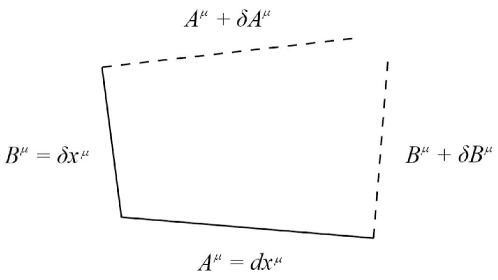
Figure 2: The breaking of the parallelogram

We considered above the arm length $L$ to be small compared to the width of the wave packet that describes the function $H$. This property was taken into account in Eqs. (31) and (32). By comparing Figs. 1 and 2 we are led to identify $a^{\mu}=dx^{\mu}$ and $v^{\mu}=\delta x^{\mu}$. Therefore,

$$T^{0}\,_{\alpha\beta}\,dx^{\alpha}\delta x^{\beta}=T^{0}\,_{\alpha\beta}\,a^{\alpha}v^{\beta}\,.$$ (41)

A straightforward calculation leads to

$$T^{0}\,_{\alpha\beta}\,a^{\alpha}v^{\beta}=T^{0}\,_{01}a^{0}v^{1}-T^{0}\,_{02}a^{2}v^{0}-T^{0}\,_{12}a^{2}v^{1}\,.$$ (42)

Taking into account the expressions of the torsion tensor components given by Eq. (38), and using $g^{00}=(-1-{1\over 2}H)$ and $g^{03}=-{1\over 2}H$, we obtain

$$T^{0}\,_{\alpha\beta}\,a^{\alpha}v^{\beta}={L^{2}\over 4}\biggl{[}{{({{\partial H}\over{\partial x}})-({{\partial H}\over{\partial y}})}\over{(1-{1\over 2}H)^{3/2}}}\biggr{]}\,,$$ (43)

and also $T^{i}\,_{\alpha\beta}\,a^{\alpha}v^{\beta}=0$, for $i=1,2,3$. Equation (43) represents precisely the breaking of the parallelogram given by Eq. (33). Note that Eq. (43) cannot be explained in terms of the curvature tensor, which depends on second order derivatives of the metric tensor.

5 The breaking of parallelograms in the $(+x,-x)$ and $(+x,-y)$ directions

In this section we will consider two types of parallelograms, geometrically distinct from the one depicted in Fig. 1, in the presence of the gravitational wave described by Eqs. (19-21). The parallelogram of Fig. 1 is characterized as a $(+x,+y)$ parallelogram. In the geometrical constructions below, the vectors $v^{\mu}$ and $w^{\mu}$ are given as in Section 2, by Eqs. (24-25). Only the vectors $a^{\mu}$ and $b^{\mu}$ will be modified. The two new parallelograms are the following.

5.1 Parallelogram in the $(+x,-x)$ directions

The light beams travel back and forth in the positive $x$ direction ($v^{\mu}$, $w^{\mu}$), and in the negative $x$ direction ($a^{\mu}$, $b^{\mu}$), along arms of equal length $L$. Thus, the vectors $a^{\mu}$ and $b^{\mu}$ are defined by

$$a^{\mu}=\biggl{(}{L\over{(1-H/2)^{1/2}}},-L,0,0\biggl{)}\,,\ \ \ \ \ H=H(x_{0}-L,y_{0},t_{0}+dt)\,,$$ (44)

$$b^{\mu}=\biggl{(}{L\over{(1-H/2)^{1/2}}},L,0,0\biggl{)}\,,\ \ \ \ \ H=H(x_{0},y_{0},t_{0}+2dt)\,.$$ (45)

The breaking of the parallelogram is given as before by $\Delta^{\mu}=(v^{\mu}+w^{\mu})-(a^{\mu}+b^{\mu})=(\Delta^{0},0,0,0)$. After a simple algebra we find

$$\Delta^{0}={L^{2}\over 2}\biggl{[}{{{{\partial H}\over{\partial x}}}\over{(1-{1\over 2}H)^{3/2}}}\biggr{]}\,.$$ (46)

The expression above is also obtained from the torsion tensor components according to

$$T^{0}\,_{\alpha\beta}a^{\alpha}b^{\beta}=T^{0}\,_{01}a^{0}v^{1}+T^{0}\,_{10}a^{1}v^{0}=\Delta^{0}\,,$$ (47)

where all quantities are given by eqs. (24), (38) and (44).

5.2 Parallelogram in the $(+x,-y)$ directions

Here we consider that the light beams travel in the positive $x$ direction ($v^{\mu}$) and in the negative $y$ direction ($a^{\mu}$), along arms of equal length $L$. The vectors $a^{\mu}$ and $b^{\mu}$ in this case are defined by

$$a^{\mu}=\biggl{(}{L\over{(1-H/2)^{1/2}}},0,-L,0\biggl{)}\,,\ \ \ \ \ H=H(x_{0},y_{0}-L,t_{0}+dt)\,,$$ (48)

$$b^{\mu}=\biggl{(}{L\over{(1-H/2)^{1/2}}},0,L,0\biggl{)}\,,\ \ \ \ \ H=H(x_{0},y_{0},t_{0}+2dt)\,.$$ (49)

Once again the breaking of the parallelogram is given by $\Delta^{\mu}=(v^{\mu}+w^{\mu})-(a^{\mu}+b^{\mu})=(\Delta^{0},0,0,0)$. After some simple calculations we find

$$\Delta^{0}={L^{2}\over 4}\biggl{[}{{({{\partial H}\over{\partial x}})+({{\partial H}\over{\partial y}})}\over{(1-{1\over 2}H)^{3/2}}}\biggr{]}\,.$$ (50)

As in the previous case, the expression above is exactly obtained from the torsion tensor components according to

$$T^{0}\,_{\alpha\beta}a^{\alpha}b^{\beta}=T^{0}\,_{01}a^{0}v^{1}+T^{0}\,_{20}a^{2}v^{0}=\Delta^{0}\,.$$ (51)

Expressions (43), (47) and (51) are in agreement with the geometrical interpretation of the torsion tensor. The latter explains the geometrical breaking of parallelograms in space-time, and is fundamental in the description of the gravitational phenomena considered in the present framework. As we mentioned earlier, the breaking of the three parallelograms cannot be explained with the help of the curvature tensor of the space-time.

6 Conclusions

The breaking of the parallelogram depicted in Fig. 1 was obtained by considering first the physical vectors $v^{\mu}$, $w^{\mu}$, $a^{\mu}$ and $b^{\mu}$, and then by analysing the parallel transport of vectors in a space-time endowed with torsion. The tetrad frame (34) and the torsion tensor components explain the breaking of the parallelogram. Therefore the measurement of the breaking of the parallelogram of Fig. 1 is, at the same time, a direct manifestation of gravitational waves and of the space-time torsion. This effect cannot be explained directly by the metric tensor, and neither as a manifestation of the curvature of the space-time.

As a consequence of Eq. (46), we observe that two events that are simultaneous in the flat space-time, may not be simultaneous in the presence of a plane-fronted gravitational wave. Two events are simultaneous in space-time if the relevant parallelogram is not broken.

The quantity $\Delta^{0}$ given by Eq. (33) has dimension of length, and is measured on the worldline of the splitting point $S$. The interval of time elapsed between the arrival at the point $S$ of the two light rays, described by $w^{\mu}$ and $b^{\mu}$, is given by $\Delta\tau=\Delta^{0}/c$,

$$\Delta\tau={L^{2}\over 4c}\biggl{[}{{({{\partial H}\over{\partial x}})-({{\partial H}\over{\partial y}})}\over{(1-{1\over 2}H)^{3/2}}}\biggr{]}\,,$$ (52)

where $c$ is the speed of light.

We emphasize that we are considering a strictly thought experiment. However, in the context of the LIGO experiment, we may obtain an expression for $\Delta\tau$. The length $L$ of one arm of the LIGO detector is $4\,km$. Assuming that the light rays perform 200 round trips along each arm (after the splitting at the point $S$ and before the detection), and also assuming the amplitude of the gravitational wave to be small, we find

$$\Delta\tau\approx(533\,m\cdot s)\biggl{(}{{\partial H}\over{\partial x}}-{{\partial H}\over{\partial y}}\biggr{)}\,.$$ (53)

Note that since $H$ is a function of $x,y$ and $u=(z-t)/\sqrt{2}$, the partial derivatives are not linearly dependent on the frequency of the incident gravitational wave.

In view of (i) the lack of sufficient knowledge about the astrophysical source of gravitational perturbations, (ii) of the small intensity of the expected gravitational waves, and (iii) of the arbitrariness of the function $H(x,y,u)$, in practice it will be difficult to distinguish the detection of a gravitational wave signal from the background noise, at least in the context of the LIGO experiment. The background noise is characterized by a pattern of random oscillations that will be the subject of precise measurements of the Fermilab Holometer experiment [20]. The latter is an experiment designed to study the properties of space-time at the smallest scales, by probing the nature of noise in the very structure of the space-time. The Fermilab Holometer is constituted by two similar interferometers, placed parallel and very close to each other, so that the measurements in both interferometers may be correlated. Although the function $H$ is not a priori known, we assume that it is given in the form of a wave packet in the direction of propagation, and believe that its presence will momentarily alter the pattern of the background noise. Therefore, sudden and unexpected changes in the background noise may indicate the passage of a gravitational wave. The Fermilab Holometer experiment might provide strong indications of the presence of non-linear waves.

References

- [1] K. Hayashi, Phys. Lett 69B, 441 (1977); K. Hayashi and T.Shirafuji, Phys. Rev. D 19, 3524 (1979); 24, 3312 (1981).
- [2] F. W. Hehl, in “Proceedings of the 6th School of Cosmology and Gravitation on Spin, Torsion, Rotation and Supergravity”, Erice, 1979, edited by P. Bergmann and V. de Sabbata (Plenum, New York, 1980).
- [3] J. W. Maluf, J. Math. Phys. 35, 335 (1994).
- [4] J. W. Maluf, Ann. Phys. (Berlin) 14, 723 (2005).
- [5] F. Gronwald, Int. J. Mod. Phys. D 6 (1997) 263.
- [6] J. Ehlers and W. Kundt, in “Gravitation: an Introduction to Current Research”, edited by L. Witten (Wiley, New York, 1962).
- [7] M. Pitkin, S. Reid, S. Rowan and J. Hough, Living Rev. Relativity 14, (2011), 5.
- [8] S. L. Danilishin and F. Y. Khalili, Living Rev. Relativity 15, (2012), 5.
- [9] E. Schucking, “Gravitation is Torsion” [arXiv:0803.4128].
- [10] J. W. Maluf and S. C. Ulhoa, Phys. Rev. D 80, 044036 (2009).
- [11] J. W. Maluf, F. F. Faria and S. C. Ulhoa, Class. Quantum Grav. 24, 2743 (2007).
- [12] J. W. Maluf and F. F. Faria, Ann. Phys. (Berlin) 17 (2008) 326.
- [13] F. H. Hehl, J. Lemke and E. W. Mielke, “Two Lectures on Fermions and Gravity”, in Geometry and Theoretical Physics, edited by J. Debrus and A. C. Hirshfeld (Springer, Berlin Heidelberg, 1991).
- [14] B. Mashhoon and U. Muench, Ann. Phys. (Berlin) 11 (2002) 532.
- [15] F. W. Hehl, J. D. McCrea, E. W. Mielke and Y. Ne’eman, Phys. Rep. 258, 1 (1995).
- [16] R. Arnowitt, S. Deser and C. W. Misner, in Gravitation: an Introduction to Current Research, edited by L. Witten (Wiley, New York, 1962).
- [17] J. W. Maluf, J. F. da Rocha-Neto, T. M. L. Toríbio and K. H. Castello-Branco, Phys. Rev. D 65, 124001 (2002).
- [18] H. Stephani, “Relativity: an Introduction to Special and General Relativity”, third edition (Cambridge Univ. Press, Cambridge, 2004).
- [19] J. W. Maluf and S. C. Ulhoa, Phys. Rev. D 78, 047502 (2008).
- [20] C. R. Hogan, “Interferometers as probes of Planckian quantum geometry”, arXiv:1002.4880 (2012) (see also astro.fnal.gov/projects/OtherInitiatives/holometer-project.html).