Numerical Studies of Particle Laden Flow in Dispersed Phase

Proceedings of Summer Program 2010

I abstract

To better understand the hydrodynamic flow behavior in turbulence, Particle-Fluid flow have been studied using our Direct Numerical(DNS) based software DSM on MUSCL-QUICK and finite volume algorithm. The particle flow was studied using Eulerian-Eulerian Quasi Brownian Motion(QBM) based approach. The dynamics is shown for various particle sizes which are very relevant to spray mechanism for Industrial applications and Bio medical applications.

II Introduction and Motivation

Particle laden flows are of great interest in Chemical, Spray Industrial applications or Biomedical applications. Knowledge of particle transport and concentration properties are crucial for experimental design of such applications. Numerical simulation coupling Lagrangian tracking in discrete carrier phase of turbulence with Direct Numerical Simulation(DNS) simulation phase provides a robust tool to investigate such flows. Many applications of this type of flow are aerosol[Nitrogen and other post combustion particles] particle flow studies in post combustion chamber for the design and performance optimization of aviation engine and also for spray mechanism in nano particle spray Industries. In studies of arterial blood flow, these simulations help to visualize the blood flow in cardio-vascular region. Numerical Simulation coupling Lagrangian approach of particle tracking along with DNS(Direct Numerical Simulation) phase of simulation provides a powerful tool for such flow such in any geometry.
In all Industrial applications of the boundary wall problem, boundaries are not smooth in true sense and the presence of roughness cause additional energy dissipation enhancing mixing in the particle-fluid mixture. Most commercial software like Fluent and CFX are unable to incorporate such physics. There are two commonly used methods to simulate fluid-particle flows:Eulerian-Lagrangian and Eulerian-Eulerian, and both of these have been used to model the settling of particles in an in compressible fluids. The Eulerian-Lagrangian technique treats the fluid as a continuous medium described by Navier-Stokes equation modified to account for the fluid-particle interaction where particles are considered as point in fluid such that Newton’s second law can be applied separately to each particle to track its motion in a Lagrangian frame of reference. Particle-particle interaction and particle-fluid interactions are modeled for each particle. When particle numbers become large, particle particle interaction and turbulence modifications become expensive to study such kind of flows. This even sometimes becomes computationally challenging to retrieve data [11]. These effects become important in the calculation which makes DNS simulation approach to become numerically Numerical computation based on separate Eulerian balance can provide very good alternative approach to such problems which are numerically not so expensive in comparison to grid size. Eulerian approach is based on separate balance equation for both phases through inter phase coupling terms. Such Eulerian-Eulerian DNS approach have been validated for the case of particles with low inertia which follow their carrier fluid almost instantaneously due to their small response time compared to integral time scale of turbulence[Druzini et al] [5]. In case of inertial particles, where particle response time scale is comparable to integral time scale, additional effects have to be taken into account. As pointed out by Fevrier et al [7] [8] calculations, particle phase transport equations must take account all dispersion effects due to local random motion which is induced by particle-particle interaction and particle-turbulence interaction. In fact, complex nonlinear particle-particle interaction exists in the vicinity of wall.
Following Fevrier et al [7], a conditional average of all dispersed phases with respect to the carrier phase flow allows the derivation of instantaneous mesoscopic particle fields and instantaneous Eulerian balance equation which can be calculated by taking into account for the effect of random motion. The detail calculation of energy dissipation parameter also takes into account of random motion of the dispersed phase.
Using forced isotropic turbulence simulations, Fevrier et al [8] showed that uncorrelated quasi Brownian motion of the particles increases with inertia(Stokes Number).
In cases where particle relaxation time is comparable to Lagrangian integral time scale, kinetic energy of the quasi Brownian motion is about 30% of total kinetic energy of the dispersed phase.
The importance of Quasi Brownian Motion(QBM) is illustrated in a preliminary test in case of decaying homogeneous isotropic turbulence. The Eulerian model is then applied to the experimental case of Snyder & Lumley [16] which has been previously simulated using Lagrangian tracking approach by Elghobashi & Trusdel [6]. This allows us to compare results of simulation with Lagrangian approach and also with the experimental data. The next section will illstrate the Eulerian model and related calculation.

III The Eulerian Model

Eulerian equations for the dispersed phase may be derived using the methods which consists of volume filtering of the separate, local instantaneous equations accounting for the inter facial jump conditions [Druzini et al[5]]. Such an averaging approach is very restrictive because particle size and inter particle distance have to be smaller than the smallest turbulence scale.
A different approach in the framework of kinetic theory is the statistical approach. In analogy to the derivation of Navier Stokes equation by non equilibrium statistics by Chapman & Cowling [2], a point probability density function(pdf) ${f_{\rm p}}{\rm{(1)}}(c_{\rm p};x_{\rm p},t)$ defining the local instantaneous probable number of particle centers with the given translation velocity $u_{\rm p}=c_{\rm p}$, is defined. This function obeys Boltzmann type of kinetic equation which accounts for the momentum exchange with carrier fluid and other inter particle forces and external nonlinear force field.
Reynold-averaged Transport equations for the first moment such as particle concentration, mean velocity and particle kinetic stress can be derived directly from this probability density function of Kinetic equation [Simonin et. al.[18]].
To derive local instantaneous Eulerian Equation in dilute flows(without turbulence modifications of the particles), Fevrier et al [8] proposed an approach that uses averaging over all dispersed phases over single carrier phase condition. Such an averaging leads to conditional particle dispersion function(pdf) for the dispersed phase defined by,

$$\check{{f_{\rm p}}^{\rm{(1)}}}(c_{\rm p};{\bf x},t,{\it H_{\rm f}})=\langle{W_{\rm p}}^{\rm 1}(c_{\rm p};x,t|H_{\rm f}\rangle$$ (1)

The $W_{\rm p}$ ’s are the position and velocities of corresponding particle with time. With this definition, one may define local instantaneous particulate velocity field defined as ”Mesoscopic Eulerian Particle Velocity Field”. This field is obtained by averaging discrete particle velocities measured at a particular position and time for all particle-flow realizations and at given carrier-phase realization.
Such an averaging leads to a conditional ”pdf” for the dispersed phase,

$$\check{u_{\rm p}}({\bf u},t,{\it H_{\rm f}})=\cfrac{1}{{\check{n_{\rm p}}}^{\rm{(1)}}}\int c_{\rm p}\check{f_{\rm p}}^{\rm{(1)}}(c_{\rm p};{\bf x},t,{\it H_{\rm f}})dc_{\rm p}$$ (2)

Here

$$\check{n_{\rm p}}^{\rm{(1)}}=\int\check{f_{\rm p}}^{\rm{(1)}}(c_{\rm p};{\bf x},t,{\it H_{\rm f}})dc_{\rm p}$$ (3)

is the mesoscopic particle number density. Application to the conditional averaging procedure to the kinetic equation governing the particle pdf directly leads to the transport equation for the first moments of number density and mesoscopic Eulerian velocity.

$$\cfrac{\partial}{\partial t}\check{n_{\rm p}}+\cfrac{\partial}{\partial x_{\rm i}}\check{n_{\rm p}}\check{u_{\rm{p,i}}}=0$$ (4)

$$\check{n_{\rm p}}\cfrac{\partial}{\partial t}\check{u_{\rm{p,i}}}+\check{n_{\rm p}}\check{u_{\rm{p,j}}}\cfrac{\partial}{\partial x_{\rm j}}\check{u_{\rm{p,i}}}=-\cfrac{\check{n_{\rm p}}}{\check{\tau_{\rm p}}^{\rm F}}[\check{u_{\rm{p,i}}}-u_{\rm{f,i}}]-\cfrac{\partial}{\partial x_{\rm j}}\check{n_{\rm p}}{\delta}\check{\sigma_{\rm{p,i,j}}}+\check{n_{\rm p}}g_{\rm i}$$ (5)

Here $\delta\check{\sigma_{\rm{p,i,j}}}$ is the mesoscopic kinetic stress tensor of the particle Quasi Brownian velocity distribution. Our calculation showed that this term is non negligible for inertial particles in turbulent flow.

III.1 The Stress Tensor of Quasi Brownian Motion(QBM)

The stress term in eqn(5) arises from the ensemble average of the non linear term in the transport equation for particle momentum,

$$\begin{split}n_{\rm p}{\partial}\check{\sigma_{\rm{p,ij}}}=\int(c_{\rm p}-\check{u_{\rm{p,i}}})(c_{\rm{p,j}}-\check{u_{\rm{p,j}}})\check{f_{\rm p}}^{\rm{(1)}}(c_{\rm p};{\bf x},t,{\it H_{\rm f}})dc_{\rm p}\\ =\check{n_{\rm p}}{\delta}u_{\rm{p,i}}\widehat{\delta u_{\rm{p,i}}}\end{split}$$ (6)

When Euler or Navier Stokes equation is derived from kinetic gas theory, the trace of ${\delta}u_{\rm p}\widehat{\delta}u_{\rm{p,j}}$ is interpreted as temperature(ignoring Boltzman constant and molecular mass) and related to pressure by equation of state.
In Euler or Navier Stokes equation, temperature is defined as the uncorrelated part of kinetic energy. And uncorrelated part of kinetic energy is defined as,

$${\partial}{q_{\rm p}}^{\rm 2}=\cfrac{1}{2}{\delta}u_{\rm{p,i}}\widehat{\delta u_{\rm{p,i}}}$$ (7)

In analogy to Euler or Navier Stokes equation, product of uncorrelated kinetic energy and particle number density is defined as uncorrelated Quasi Brownian Pressure(QBP) as,

$$\check{P_{\rm p}}=\check{n_{\rm p}}\cfrac{2}{3}{\delta}{q_{\rm p}}^{\rm 2}$$ (8)

When particle number density becomes non uniform, as in the case of compressible gas, the pressure tends to homogenize particle number density.
The non diagonal part of stress tensor can be identified in analogy to Navier Stokes Equation as viscous term($\Theta_{\rm{ij}}$). The momentum transport equation (5) becomes,

$$\check{n_{\rm p}}\cfrac{\partial}{\partial t}\check{u_{\rm{p,i}}}+\check{n_{\rm p}}\check{u_{\rm{p,j}}}\cfrac{\partial}{\partial x_{\rm j}}\check{u_{\rm{p,i}}}=-\cfrac{\check{n_{\rm p}}}{\check{\tau_{\rm p}}^{\rm F}}[\check{u_{\rm{p,i}}}-\check{u_{\rm{f,i}}}]-\cfrac{\partial}{\partial x_{\rm i}}\check{P_{\rm p}}+\cfrac{\partial}{\partial x_{\rm j}}{\theta}_{\rm{i,j,p}}+n_{\rm{p}}g_{\rm i}$$ (9)

Moreover, it can be shown mathematically that equation (9) without pressure like term leads to nonphysical solution.

III.2 Simulation with and without QBM

Preliminary simulations were performed without any stress term related to QBM. Particles tend to accumulate rapidly in smaller region causing unnecessary high particle number density. This causes numerical simulation to fail. In order to ensure that failure is not caused by numerical problem, different simulations with different Reynold Number was carried out showing same result.
Simulations with quasi Broqnian pressure(QBP) and without quasi Brownian viscous stress were done on the above test cases. Fevrier et al [8] measured in forced homogeneous isotropic turbulence, a mean quasi Brownian kinetic energy $\partial q^{\rm 2}$ proportional to the mean mesoscopic kinetic energy ${\check{q_{\rm p}}}^{\rm 2}=\cfrac{1}{2}\langle\check{u_{\rm{p,i}}}{\check{u_{\rm{p,i}}}}\rangle$ with a proportionality coefficient depending on the Stokes number.
The relation between the quasi Brownian kinetic energy and mean resolved kinetic energy is used,

$${\delta}{q_{\rm p}}^{\rm 2}=5{\check{q_{\rm p}}}^{\rm 2}$$ (10)

Such a QBP model allows all the test cases that failed without quasi Brownian stress term to simulate. Compared to the value obtained by Fevrier et al [8], relation (10) overestimates the quasi Brownian kinetic energy. When viscous stress term is incorporated in the calculation, it reduces the pressure.
In order to quantify the effect of particle confinement, the normalized variance of particle number density is introduced,

$$g(r,t)=\cfrac{\langle n(x,t)n(x+r,t)\rangle}{{\langle(n(x,t)\rangle}^{\rm 2}}$$ (11)

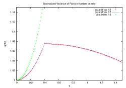
Figure 1: Fig 1. Normalized variance distribution of particle number density without QBP(green color) and with QBP(red color)

Figure 1 compares time evolution of $g(0,t)$ from simulations with and without QBP. The quasi Brownian pressure is found to affect the particle conglomeration or segregation significantly.
Figure 2 shows kinetic energy spectra of the carrier phase and the dispersed phase with and without QBP. Our simulations show same behavior of simulations that without QBP case, particle kinetic energy of small scale turbulence becomes larger than the carrier phase in contrast to the results of Fevrier et al [8]. This is probably due to nonphysically large particle accumulation in the carrier phase of turbulent flow which is the region of high shear strain and low vorticity. The vorticity development can be another useful tool to study such flows. Figure 5 shows the vorticity development for the carrier phase as well as dispersed phase. In presence of QBP contribution limiting particle segregation, particle enstrophy behavior shows similar effect. Figure 3 shows particle enstrophy distribution with and without QBP. The quasi Brownian viscous term plays a major role by inducing a strong small scale strong dissipation effect in addition to drag force. Figure 3 shows the effect by characterizing the temporal increase of enstrophy function.

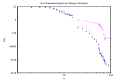
(a) Fig 2. non dimensional energy spectra of $\dotplus(red)$ carrier phase $\diamond(pink)$ without QBM and $\times(blue)$ with QBM

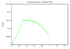
(b) Fig 3. Enstrophy distribution in dispersed phase—-with $\times(green)$ and without $\dotplus$ QBP

IV Particle dynamics and dispersion

Particle dispersion in Lagrangian simulations is usually measured by tracking individual particle path and calculating the variance of the relative displacement. In our simulation, Eulerian-Eulerian simulation was performed with one way coupling. We also studied particle dynamics in simulations with gravity and without gravity to study the gravitational effect on dynamics with nonlinear force. The Eulerian-Eulerian simulation was carried out in a coupled way so that carrier phase turbulence affects the dispersed phase through particle dynamics. The interaction in the momentum equation is drag force and nonlinear Basset force in the limit of large density ratio $\rho_{\rm p}/\rho_{\rm f}$.
The characteristic relaxation time is computed by formulation,

$$\langle{X_{\rm p}}^{\rm 2}(t)\rangle=\cfrac{1}{N}{\sum_{\rm{j=1}}}^{\rm N}{\{x_{\rm{p,j}}(t)-x_{\rm{p,j}}(t_{\rm 0})\}}^{\rm 2}$$ (12)

The characteristic polynomial of the Jacobian Matrix is given by,

$$(u-\lambda)\left((u-\lambda)(u-\lambda)-\cfrac{\gamma P}{\rho}\right)(\check{u_{\rm p}}-\lambda)\left((\check{u_{\rm p}}-\lambda)(\check{u_{\rm p}}-\lambda)-\cfrac{\cfrac{5}{3}P_{\rm{QB}}}{\check{n_{\rm p}}}\right)=0$$ (13)

Particle dispersion can then be related to the time derivative of the quantity [13]

$${D_{\rm{p}}}^{\rm L}(t)=\cfrac{1}{2}\cfrac{d}{dt}\langle{X_{\rm p}}^{\rm 2}(t)\rangle$$ (14)

Eulerian simulation can not track individual particle path. Particle dispersion is measured by semi-empirical method [13] If the simulation is being carried out with colored particles and transport equation is written in terms of ratio of colored particles to total particles $(\check{c}=\cfrac{\check{n_{\rm c}}}{\check{n_{\rm p}}})$. Then we can write transport equation as,

$$\cfrac{\partial}{\partial t}\check{c}\check{n_{\rm p}}+\cfrac{\partial}{\partial x_{\rm i}}\check{c}\check{n_{\rm p}}\check{u_{\rm{p,i}}}=\cfrac{\partial}{\partial x_{\rm i}}$$ (15)

Here ${\check{u_{\rm{p,i}}}}^{\rm c}$ is the mesoscopic velocity of colored particles. Since only the velocity of total particle is resolved, the right hand side term takes into account of the slip velocity between colored and mesoscopic velocity of the particle ensemble. Comparing to Navier-Stokes equation, this term is equivalent to molecular diffusion. Since slip velocity arises only from uncorrelated movement of particles, this term can be modeled as diffusion term related to quasi brownian motion. If the ensemble averaged mean number density fraction of colored particles $\langle\check{n_{\rm p}}\rangle C=\langle\check{n_{\rm p}}\check{c}\rangle$ is uniformly stratified in the $\it k$ direction[here in $-k$ direction] $\check{c}=C+\acute{c}$ and fluctuations are assumed periodic with respect to the computer domain, then fluctuation number density of colored particles $\acute{c}\tilde{n_{\rm p}}$ can be calculated from the total colored particle density function. One obtains a transport equation for the fluctuation of colored particle concentration as,

$$\cfrac{\partial}{\partial t}\acute{c}\check{n_{\rm p}}+\cfrac{\partial}{\partial x_{\rm i}}\acute{c}\check{n_{\rm p}}\check{u_{\rm{p,i}}}=-\check{n_{\rm p}}\check{u_{\rm{p,k}}}\cfrac{\partial}{\partial x_{\rm k}}C+\cfrac{\partial}{\partial x_{\rm i}}\check{c}\check{n_{\rm p}}(\check{u_{\rm{p,i}}}-{\check{u_{\rm{p,i}}}}^{\rm c})$$ (16)

Averaging the colored number density equation (15), one obtains Reynold averaged type transport equation,

$$\cfrac{\partial}{\partial t}\langle\check{n_{\rm p}}\rangle C+\cfrac{\partial}{\partial x_{\rm i}}\langle\check{n_{\rm p}}\rangle C\langle\check{u_{\rm{p,i}}}\rangle_{\rm p}=-\cfrac{\partial}{\partial x_{\rm i}}\langle\check{n_{\rm p}}\acute{c}u_{\rm{p,i}}\rangle+\cfrac{\partial}{\partial x_{\rm i}}\langle\check{c}\check{n_{\rm p}}(\check{u_{\rm{p,i}}}-{\check{u_{\rm{p,i}}}}^{\rm c})\rangle$$ (17)

Particle dispersion term can be derived by making gradient assumption,

$$(\langle\acute{c}\check{n_{\rm p}}\check{u_{\rm{p,k}}}\rangle=\langle\check{n_{\rm p}}{D_{\rm{p,k}}}^{\rm t}\cfrac{\partial}{\partial x_{\rm k}}C\rangle$$ (18)

A semi empirical diffusion coefficient can be defined as,

$${D_{\rm{p,k}}}^{\rm t}=\cfrac{\langle\check{n_{\rm p}}\acute{c}u_{\rm{p,k}}\rangle}{\langle\check{n_{\rm p}}\rangle\cfrac{\partial}{\partial x_{\rm k}}C}$$ (19)

This dispersion coefficient is comparable to the Lagrangian Dispersion coefficient(13) in the long time limit of stationary turbulence. Simulations without QBP likely underestimates Lagrangian dispersion. The characteristic particle relaxation time is computed by the formulation given by,

$$\tau_{\rm p}=\cfrac{\rho_{\rm p}d^{\rm 2}}{18f(Re_{\rm p}){\mu}}$$ (20)

Particle Reynold number for the drag force correction $f(Re_{\rm p})$ is based

$$f(Re_{\rm p})=1+0.15{Re_{\rm p}}^{\rm{0.687d0}}$$ (21)

V Numerical Simulations and results

Particle dynamics and particle dispersion have been studied by experiments and Lagrangian computations. Experimental results of Snyder & Lumley [16](referred as SL) is very robust test case for numerical simulation. They inserted particles with different inertial properties into grid generated spatially decreasing turbulence and measured particle dynamics as well as particle dispersion. The test case has been computed with Lagrangian approach by Elghobashi & Truesdell(ET) [6] . The carrier phase was taken as a temporarily decreasing homogeneous isotropic turbulence corresponding to the grid generated turbulence of SL. After an initial calculations for two turnover time $(t=\cfrac{l_{\rm{ii}}}{\acute{u_{\rm f}}})$, particles were inserted into the flow. Particle dynamics and dispersion were analyzed by ET [6] on particles similar to the experiments of Snyder & Lumley [16] for direct comparison with lagrangian simulation. We carried out particle simulation with Eulerian-Eulerian approach and comparison with the experimental results and Lagrangian simulation results were attempted. The simulations were performed on $100^{\rm 3}$ grid.
The carrier phase velocity is initialized at dimensionless time T=0 with a divergence velocity field(continuum condition) such that the kinetic energy satisfies the spectrum [6]

$$E(k,0)=\cfrac{3}{2}{\acute{u_{\rm{f,0}}}^{\rm 2}}\cfrac{k}{k_{\rm p}}\exp((-k/k_{\rm p})$$ (22)

where $\acute{u_{\rm f}}$ is the dimensionless rms velocity, k is the wave number and $k_{\rm p}$ is wavenuber of peak energy. All wave number were normalized with $k_{\rm{min}}$. In the present simulation, properties of carrier phase was validated against the properties of carrier phase turbulence of SL and ET. The spatial evolution of the flow in the experiment of SL is converted to a temporal evolution of the flow by $t=\cfrac{x}{\check{U}}$ . here $\check{U}$ is the mean convection velocity in the experiment.
Figure 4 shows dimensionless velocity square in the carrier phase in comparison with Lagrangian simulation(ET) and experiment(SL) results.

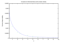
(c) Fig 4. Squared dimensionless velocity Distribution–Lagrangian ($\times$) and present(—) simulation

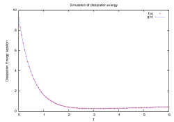
(d) Fig 5. Comparison of dissipation energy in carrier phase with Lagrangian simulation

To verify numerical simulation resolution, dissipation energy $\epsilon$ is also compared to the temporal change of kinetic energy $\cfrac{d}{dt}{q_{\rm f}}^{\rm 2}$ in Figure 5. Our result shows excellent agreement between dissipation and kinetic energy decrease. So it can be assumed that numerical dissipation is negligible compared to viscous dissipation.
In Figure 6, Reynold number from our simulation with Lagrangian simulation. The present simulation more rapid decay of turbulent Reynold number compared to the Lagrangian simulation(ET).

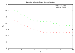
(e) Fig 6. Evolution of Reynold Number in carrier phase $\times(green)$ Lagrangian and $\dotplus(red)$ present simulation

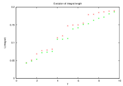
(f) Fig 7. Evolution of integral length scale $\times(pink)$..Lagrangian and $\dotplus(green)$ ..present simulation

This is because the integral length scale increase slowly in our simulation(Figure 7). The temporal evolution of integral time length scale shows similar qualitative behavior in eulerian simulation. Particles were inserted as in the Lagrangian simulation ${{u_{\rm f}}^{\rm\prime}}^{\rm 2}$ (ET) at nondimensional time $T=2.0$ with same velocity as carrier phase when inserted into the turbulent flow. Particle properties were analyzed in turbulence with and without gravity. When particles are inserted into gravity, they establish a mean terminal velocity vertically downward direction. The gravity constant was calculated as in the experiment. For all types of particle sizes, relative square velocity in the present simulation shows same qualitative behavior as in the Lagrangian simulation. Figure 8 and 9 shows the squared relative velocity distribution of the carrier phase without and with the presence of gravity. The gravity constant is measured such that same ratio of $\cfrac{v_{\rm{t,0}}}{u_{\rm 0}}$. In all cases, present simulation shows same behavior as Lagrangian simulation. We have chosen temporarily decaying turbulence condition in our simulation as initial parameter. In Eulerian simulations, one does not have access to individual particle paths. Particle dispersion can still be measured by a semi-empirical method [13]. Since only the velocity of the total droplet number is resolved which brings another extra term on right hand side of the above equation. This term takes into account the slip velocity between colored particle and the mesoscopic velocity of particle ensemble.

dispersed phase in excellent agreement. It is observed in the present simulation that when gravity is taken into account, particle dynamics was modified. The observed crossing trajectory effect is due to mean settling velocity of the particle and leads to decrease in integral time scale of fluid turbulence. Such an effect leads to an increase of effective particle stokes number. This also increases the relative squared velocity value with respect to the non settling value. Particle dispersion is also calculated for the dispersed phase. In order to compare with the carrier phase, equation (16) is solved for carrier phase without molecular diffusion. In the Eulerian simulation with gravity taking into account, particle dispersion is significantly lower than the simulation without gravity consistent with Csanady analysis [3]. Calculation for all particles show that Eulerian simulation shows similar qualitative behavior as Lagrangian simulation and dispersion calculation is quantitatively lower than Lagrangian simulation.

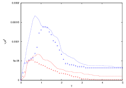
(g) Fig 8. Evolution relative velocity(dimensionless) with gravity

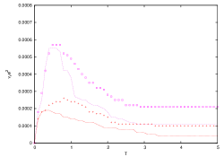
(h) Fig 9. Evolution of relative velocity(dimensionless) without gravity

The Eulerian equations for the dispersed phase have been implemented on the slip velocity

$$Re_{\rm p}=\cfrac{|{\vec{u_{\rm p}}-\vec{u_{\rm f}}|}d}{\nu_{\rm f}}$$ (23)

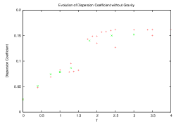
(i) Fig 10. Evolution of dispersion coefficient without gravity

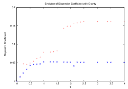
(j) Fig 11. Evolution of dispersion coefficient with gravity

The Eulerian mean square relative velocity differs from the Lagrangian mean square velocity by the quantity $\delta{u_{\rm p}}^{\rm 2}$ from QBM. Figure 12 shows the temporal development of the carrier phase ${u_{\rm f}}^{\rm 2}$. Balakin et al [1] also studied uniformly sized sediment particle movements in viscous fluids using Eulerian-Eulerian simulation and compared with experimental results of Nicolai et. al [14] for sedimenting particles. They corresponding governing equation is given by,

$$\cfrac{\partial(\alpha_{\rm m}\rho_{\rm m})}{\partial t}+\bigtriangledown(\alpha_{\rm m}\rho_{\rm m}\vec{u_{\rm m}})=0$$ (24)

Index ${\it m}$ assigns the phase(liquid or solid), $\alpha$ is the volume fraction, $\rho$ is the density and $\vec{u}$ is mean phase velocity. The momentum equation is given by,

$$\cfrac{\partial(\alpha_{\rm m}\rho_{\rm m}\vec{u_{\rm m}})}{\partial t}+\bigtriangledown(\alpha_{\rm m}\rho_{\rm m}\vec{u_{\rm m}}\vec{u_{\rm m}})=-\alpha_{\rm m}\vec{\bigtriangledown}p+\alpha_{\rm m}\rho_{\rm m}\vec{g}+\bigtriangledown(\alpha_{\rm m}\tau_{\rm m})+\vec{M_{\rm m}}+\vec{F_{\rm A}}$$ (25)

In further to investigate our simulation approach, we carried out simulation for sedimenting particle flow simulation similar to the experiment done by Nicolai et al. [14] Figure 11 shows the comparison between our simulation with Experimental results of Nicolai etl al. [14] and also Balakin et al [1] simulation results. The dispersed phase velocity is plotted against volume fraction of carrier phase to dispersed phase. Our simulation strongly agree with experimental data.

(k) Fig 12: Time average settling velocity plotted as a function of solid volume fraction, red $\times\cdots$ (Nicolai et al), blue $\times\cdots$ balakin et al and green $\circ\cdots$ (our simulation)

.

VI Conclusion

Particle dispersion is measured for the dispersed phase. In order to compare with the carrier phase, the equivalent of equation(16) is solved for carrier phase without molecular diffusion. A preliminary model of Quasi Brownian Motion was used to study unresolved kinetic particle energy. This model allowed simulations to compare with the experimental results of Snyder & Lumley [16]. We also have done for sedimenting particles similar to experiment done by Nicolai et. al [14] and compared with Balakin simulation results. [1] which strongly shows that Quasi Brownian ensemble approach is very strong alternative tool for two phase flow modeling.

References

- [1] Balakin B.V, Hoffman A.C, Kosinski P.J & Rhyne L.D; Eulerian-Eulerian CFD model for the sedimentation of spherical particles in suspension with high particle concentration, Engineering Applications of Computational Fluid mechanics,4(1), 2010,116-126.
- [2] Chapman S. & Cowling T.G, The Mathematical Theory of Non-Uniform Gases, Cambridge University Press.
- [3] Csanady G.T; Turbulent Diffusion of Heavy Particles in Atmosphere, J. Atmos. Science 20 1963, 201-208.
- [4] Drew O.A & Passman S.L; Theory of Multicomponent Fluids, Springer Series in Applied Mathematical Sciences 135, 1998.
- [5] Druzhini O.A & Passman S.L; On the decay Rate of Isotropic Turbulence with Micro-Particles, Phys Fluids 11,1999, 602-610.
- [6] Elgobashi S. & Truesdell G.C; Direct Simulation of Particle Dispersion in a Decaying Isotropic Turbulence, J. Fluid Mech 242, 1992,655-700.
- [7] Fevrier P. & Simonin O.; Statistical and Continuum Modeling of Turbulence Reactive Particulate Flows, Part 2, In Theoretical and Experimental Modeling of Particulate Flows, Lecture Series, 2000-06, von Karman Institute for Fluid Dynamics.
- [8] Fevrier P., Simonin O. & Squires K.D; Partioning of particle velocities in gas-solid flows into a continuous field and a spatially-uncorrelated random distribution: theoretical formalism and numerical study, J. Fluid Mech.,533, 2005,1-46.
- [9] Fuchs N.A. (1964); The mechanics of Aerosol, Dover, Mineola, NY.
- [10] Hogan R.C & Cuzzi J.N; A Cascade Model for Particle Concentration and Enstrophy in Fully developed Turbulence with Mass Loading Feedback, axXiv:0704.1910v2 [astro-ph] 13 Apr,2007.
- [11] Kosinski D.M & Matsuoka A.; Modelling of dust lifting using the Lagrangian approach International Journal of Multiphase Flow,31,2005,1097-1115.
- [12] Le Veque R.J. ; Numerical Methods for Conservation Laws, Birkhaser, Boston,1996.
- [13] Monin A.S & Yaglom A.M.; Statistical Fluid Mechanics,Vol 1, MIT Press, Cambridge,MA, 1987.
- [14] Nicolai H., Herzhaft B., Hinch E.J, Oger L., Guazelli E. & Guazelli G.; Particle Velocity Fluctuations and Hydrodynamic Self-Diffusion of Sedimenting non-Brownian Spheres, it Phys. Fluids 7(1),1995, 12-33.
- [15] Reeks M.W.; On a Kinetic Equation for the Transport of Particles in Turbulent Flows, Phys Fluids A 3, 1991, 446-456.
- [16] Snyder W.H & Lumley J.L.; Some Measurements of Particle Velocity Correlation Functions in an Turbulent Flow, J. Fluid Mech. 48,1971, 41-71.
- [17] Schnfeld T. & Rudyard M.; Steady and Unsteady Flow Simulations using the Hybrid Flow Solver AVBP, AIAA J. 37,1999, 1378-1385.
- [18] Simonin O.; Combustion and Turbulence in Two Phase Flows, VKI Lecture Series 1996-02,1996.