Supplemental Material for “High Contrast X-ray Speckle from Atomic-Scale Order in Liquids and Glasses”

Abstract

This supplemental material gives additional detail on Experimental Methods and Hard X-ray FEL Source Characteristics, Calculation of Maximum Speckle Contrast, Extracting Contrast of Weak Speckle Patterns, Estimated Temperature Increase from X-ray Absorption, Split-Pulse XPCS Feasibility, and Sample Disturbance During Single Pulses.

I Experimental Methods and Hard X-ray FEL Source Characteristics

All data presented are from experiment L264, which was one of the first hard x-ray experiments at LCLS, and used the first available hard x-ray instrument (XPP). Improvements can thus be expected in future experiments due to accumulating experience in operating the LCLS to produce hard x-rays, and use of the new XCS instrument designed for XPCS measurements.

A double-crystal Si (111) monochromator was used to select a photon energy of 7.99 keV. Incident x-ray pulse energies (photons per pulse) were determined from the IPM2 monitor downstream of the monochromator but upstream of the attenuators, calibrated against an x-ray pulse power meter placed at the sample position. When attenuators were used, the calculated attenuation factors were applied to determine the pulse energy $\langle I_{0}\rangle$ incident on the sample. Beryllium compound refractive lenses with a focal length of 4 m were used to focus the beam to a $1.6\times 1.7~{}\mu$m H$\times$V FWHM spot at the sample position. The focal spot size was measured by scanning slit edges across the attenuated beam. The stability of the focal spot position was $0.25\times 0.37~{}\mu$m H$\times$V FWHM based on an analysis of the downstream signal fluctuations observed with the slit edges cutting half of the beam.

The sample was mounted in a helium-filled chamber. For the liquid Ga, a 2.8-mm diameter hemispherical droplet was mounted on a heated substrate, with the beam impinging upstream of and below its apex to produce an approximately symmetric reflection scattering geometry. For the Ni₂Pd₂P glass, a sample with a polished surface inclined at 15 degrees was used to give an approximately symmetric reflection scattering geometry. For the B₂O₃ glass, a fiber of diameter $18~{}\mu$m was suspended across an aperture and positioned in transmission geometry. On each sample, several locations were investigated, and data from different locations were typically combined in the analysis. For the unattenuated single-pulse Ni₂Pd₂P data, where intense pulses would permanently damage the surface (see the final section below), the sample was displaced by 40 $\mu$m every 1 or 5 pulses so as to scatter from a new sample region. A long-focal-length microscope fitted with a video camera allowed real-time observation of sample damage by the focused x-ray beam. Scattering experiments were carried out with a CCD detector having a direct-x-ray-detection deep-depletion silicon sensor with $1340\times 1300$ pixels $20~{}\mu$m square, mounted so that it could be positioned in a vertical scattering plane at various distances $L$ from the sample. Helium flight paths were used for longer detector distances.

The free electron laser parameters used were 250 pC bunch charge, a 70 fs electron beam integral pulse width, and a 60 Hz repetition rate. The machine monitors typically reported $2\pm 1$ mJ nominal pulse energy integrated over the full x-ray photon energy spectrum. A taper was introduced into the final segments of the undulator which was observed to optimize the monochromatic x-ray pulse energy. To accommodate the $\sim 2$ second readout time of the CCD without the availability of a detector shutter, we operated the LCLS in “burst mode”, where a burst containing a specified number of electron pulses (at a 60 Hz repetition rate) could be delivered to the undulator, with timing coordinated so that the CCD image could be recorded between bursts. Including the overhead associated with handshaking between various components of the x-ray source and data acquisition system, the maximum rate at which CCD patterns from a sequence of bursts could be recorded (even with single pulses) was one per six seconds.

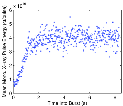
Figure 1: (Supplemental) Mean monochromatic x-ray pulse energy (photons per pulse) averaged over 50 bursts, as a function of time into each 500-pulse burst. The initial pulses in a burst were typically much weaker than later pulses.

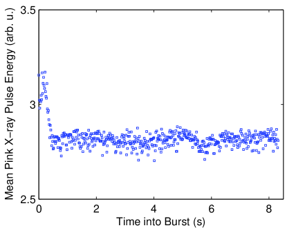
Figure 2: (Supplemental) Mean pink (un-monochromated) x-ray pulse energy averaged over 50 bursts, as a function of time into each 500-pulse bust. In contrast to the monochromatic results, the initial pink x-ray pulses in a burst have about 10% more pulse energy.

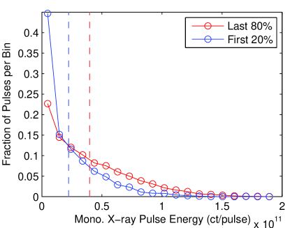
Figure 3: (Supplemental) Histogram of monochromatic x-ray pulse energies in last 80% and first 20% of burst, for fifty 500-pulse bursts. Both show distributions peaked at zero. Maximum pulse energies were about 5 times larger than the mean pulse energies (given by vertical dashed lines).

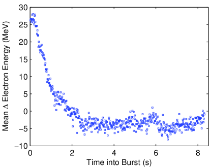
Figure 4: (Supplemental) Mean deviation (in MeV) of nominal electron beam energy in undulator from its global average of 13,426 MeV, as determined by the electron beam L3 monitor, averaged over 50 bursts, as a function of time into each 500-pulse burst. The nominal electron energy of the initial pulses in a burst deviated by about 30 MeV from its eventual value.

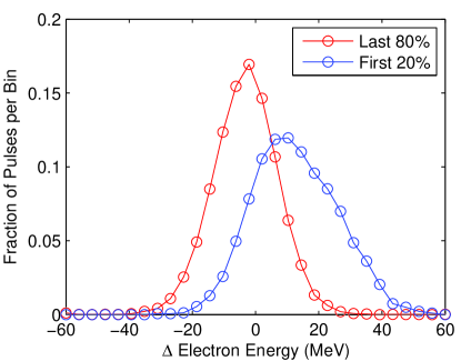
Figure 5: (Supplemental) Histogram of electron beam energy deviation of each pulse in last 80% and first 20% of burst, for fifty 500-pulse bursts. The width of the former distribution is 22 MeV FWHM.

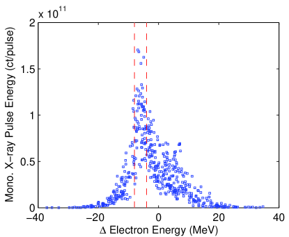
Figure 6: (Supplemental) Monochromatic x-ray pulse energy plotted vs. electron beam energy deviation for pulses in a single 500-pulse burst. Vertical dashed lines show the electron energy range used to select the pulses histogrammed in Fig. 8 (Suppl.).

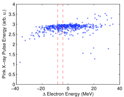
Figure 7: (Supplemental) Pink (un-monochromated) x-ray pulse energy plotted vs. electron beam energy deviation for pulses in a single 500-pulse burst. Vertical dashed lines show the same electron energy range as in Figure 6 (Suppl.).

Non-optimal machine tuning of burst mode during this experiment resulted in lower average monochromatic x-ray pulse energy for bursts of fewer than about 100 pulses than for longer bursts. The average energy of the LCLS electron beam is stabilized by a feedback loop, and different signals are used depending on whether or not x-rays are being produced during a burst. During this experiment, these signals were not properly calibrated against each other, resulting in a transient change in the average electron beam energy at the beginning of bursts. While this problem was later diagnosed and a method of calibrating the signals to eliminate the transient and obtain high x-ray pulse energy in short bursts was implemented for later experiments, we describe the problem here to explain why our single-pulse results have lower than optimal incident intensity.

Figure 1 (Supplemental) shows the mean monochromatic x-ray pulse energy as a function of time during 500-pulse bursts, averaged over 50 bursts. (Data shown in this section are from run 206, and are typical of all runs in this experiment.) On average, the initial pulses in a burst were significantly less intense than later pulses despite the fact that the un-monochromated (pink) x-ray pulse energies were initially higher than average, as shown in Fig. 2 (Suppl.). This indicates that the initial pulses had a different average photon energy than later pulses. Figure 3 (Suppl.) shows the distribution of the monochromatic x-ray pulse energies, for both the initial 100 and final 400 pulses of 500-pulse bursts. Both show distributions peaked at zero; the mean shown by the vertical dashed line was higher for the later pulses.

The transient in the monochromatic x-ray pulse energy at the beginning of a burst is related to the energy of the electron beam in the undulator. Figure 4 (Suppl.) shows the nominal electron beam energy as a function of time during the bursts, averaged as in Fig. 1 (Suppl.), while Fig. 5 (Suppl.) shows the distribution of nominal electron beam energies in each pulse for the initial 100 and final 400 pulses in a burst, corresponding to Fig. 3 (Suppl.). The mean electron beam energy changed by about 30 MeV, or 0.22%, at the beginning of each burst. The width of the nominal electron energy distribution given by the last 80% of the burst is 22 MeV FWHM, or 0.16%. Because the first harmonic photon energy emitted by the undulator scales as the square of the electron beam energy, the 0.22% change in mean electron beam energy would produce a 0.44% change in the mean x-ray photon energy, which is large compared to the 0.1% bandwidth of the first harmonic. This produced a significant change in the x-ray pulse energy at the photon energy selected by the monochromator; the net effect on this experiment was that the average available pulse energy was about $1\times 10^{10}$ photons per pulse in our single pulse data, and about $4\times 10^{10}$ photons per pulse in our 500-pulse data.

The wide variation in monochromatic x-ray pulse energy evident in Fig. 3 (Suppl.) is also due to variations in the electron beam energy, because the 0.16% FWHM pulse-to-pulse fluctuations in the nominal electron beam energy observed after the transient will produce a 0.32% fluctuation in the x-ray photon energy that is larger than the 0.1% photon energy bandwidth of each x-ray pulse. Figure 6 (Suppl.) shows the monochromatic x-ray pulse energy plotted against the nominal electron beam energy deviation from 13.426 GeV, for each pulse in a 500-pulse burst. There is a strong correlation, with a peak at about -6 MeV and a shoulder at about +6 MeV. Figure 7 (Suppl.) shows the corresponding pink x-ray pulse energies plotted in the same way; the lack of correlation indicates that it is not the number of x-ray photons, but the mean photon energy in a pulse that varies to produce the peak in Fig. 6 (Suppl.). Since the overall width of this peak is broader than the 6.7 MeV (0.05%) FWHM expected if all electrons in a pulse had the same energy, it primarily reflects the distribution of electron energies within each pulse. The distribution is inverted; e.g. the shoulder at higher nominal electron beam energy arises from electrons with lower-than-nominal energy.

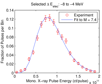
Figure 8: (Supplemental) Histogram of monochromatic x-ray pulse energy of pulses selected to have a nominal electron beam energy deviation in the range -8 to -4 MeV, for 50 bursts. Curve shows fit to Gamma distribution with mode number $M=7.4$.

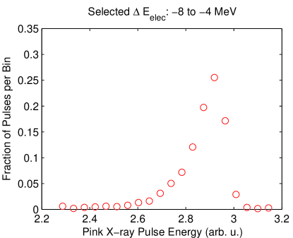
Figure 9: (Supplemental) Histogram of pink (un-monochromated) x-ray pulse energies from the electron beam energy range indicated in Fig. 7 (Suppl.).

If we select pulses having a nominal electron beam energy within a narrow range, the distribution of monochromatic x-ray pulse energies reflects the distribution expected from the SASE FEL process, where the x-ray photon energy spectrum contains many “spikes” that vary from pulse to pulse. Figure 8 (Suppl.) shows such a distribution, for nominal electron beam energies between -8 and -4 MeV (covering the peak in Fig. 6 (Suppl.)). The x-ray pulse energy distribution is no longer maximum at zero, as in Fig. 3 (Suppl.), and can be fit by a Gamma distribution NB

$$P_{\Gamma}(I)=\frac{M^{M}I^{M-1}}{\Gamma(M)\bar{I}^{M}}\exp(-MI/\bar{I})$$ (1)

with a temporal mode number of $M=7.4$. This can be compared with the simple calculation of 18.5 modes for a Si (111) bandwidth ($1.4\times 10^{-4}$ FWHM or 1.1 eV at 7.99 keV) compared to a spike width of $\Delta E=h/\Delta\tau=5.9\times 10^{-2}$ eV using $\Delta\tau=70$ fs from the electron pulse integral width. While this is consistent with an effective x-ray pulse width that is about 40% of the 70 fs electron pulse width, in rough agreement with other results GuttPRL2011 ; YoungNat2010 ; DuestererNJP2011 , the fit value of $M$ is a lower limit to the number of temporal modes in the x-ray beam (and thus the inferred x-ray pulse width is a lower limit) because of other potential contributions to the width of the x-ray pulse energy distribution. The pink x-ray pulse energies corresponding to the same -8 to -4 MeV electron beam energy range are histogrammed in Figure 9 (Suppl.) and show a much more narrowly peaked distribution.

II Calculation of Maximum Speckle Contrast

To perform XPCS on femtosecond time scales, which are much faster than the time resolution of imaging detectors, a pulse split-and-delay technique has been proposed First_Experiments ; GruebelNIM2007 ; GuttOE2009 in which the correlation time of the sample structure is determined from the change in contrast of the sum of two speckle patterns, as a function of the delay time between the patterns. This is based on a property of speckle patterns – the number of modes in a sum of equal photon density speckle patterns is given by the sum of the number of modes in all the patterns if they are uncorrelated, while it is equal to that of an individual pattern if they are fully correlated NB . Since the contrast factor $\beta$ is the inverse of the number of modes, if we record the sum of two speckle patterns of contrast factor $M_{0}^{-1}$ from two equal-energy x-ray pulses separated by a time $\tau$, the contrast factor of the sum will drop from $M_{0}^{-1}$ to $(2M_{0})^{-1}$ as $\tau$ is varied from much less than to much more than the correlation time of the sample dynamics GruebelNIM2007 .

Since measuring speckle contrast is critical to ultrafast XPCS, our experimental conditions were chosen to give high contrast from the atomic-scale order in the samples. This places conditions on the transverse and longitudinal coherence of the incident beam and the angular resolution of the detector PuseyReview ; SuttonReview . Here we describe calculations of the maximum contrast factor $\beta_{calc}$ we would expect to observe from a static sample under our experimental conditions. We can obtain an analytical formula for $\beta_{calc}$ in terms of experimental parameters such as x-ray bandwidth, beam size and detector geometry by considering the ratios between the experimental resolutions in reciprocal space and those required to fully resolve the speckle structure.

Since the transverse coherence length of the incident x-ray beam from LCLS is expected to be the full size of the beam, we simply assumed that the transverse coherence requirements are fully met and do not contribute to decreasing $\beta_{calc}$ (increasing $M$). This neglects any potential effects of aberrations in the beamline optics. (Our observation of contrast factors approaching 90% of the calculated $\beta_{calc}$ values indicates that such effects are indeed small.)

The shape of a “speckle” (i.e. signal correlation volume) in reciprocal space can be calculated from the shape of the scattering volume in real space. This can be described by $t$, the effective length of the scattering volume along the beam direction, and $s_{v}$ and $s_{h}$, the transverse beam sizes (FWHM) in and out of the scattering plane, respectively. The non-zero photon energy bandwidth of the incident beam $\Delta E/E$ gives an experimental resolution in the radial direction of $\delta Q_{r}^{exp}=(\Delta E/E)Q$. For transmission geometry, the speckle correlation volume in reciprocal space is an ellipsoid with diameters $2\pi/t$, $2\pi/s_{v}$, and $2\pi/s_{h}$, tilted at the Bragg angle $\theta=\sin^{-1}(Q\lambda/4\pi)$ with respect to the radial direction, so its radial width is $\delta Q_{r}^{sp}=2\pi/(s_{v}^{2}\cos^{2}\theta+t^{2}\sin^{2}\theta)^{1/2}$. For symmetric reflection geometry, this expression simplifies to $\delta Q_{r}^{sp}=2\pi/(t\sin\theta)$. The factor by which $M$ is increased due to the non-zero radial resolution can be expressed as $M_{rad}=[1+(\delta Q_{r}^{exp}/\delta Q_{r}^{sp})^{2}]^{1/2}$, which for transmission geometry gives

$$M_{rad}^{tr}=\left[1+\frac{Q^{2}(\Delta E/E)^{2}(s_{v}^{2}\cos^{2}\theta+t^{2}\sin^{2}\theta)}{4\pi^{2}}\right]^{1/2}$$ (2)

and for symmetric reflection geometry gives

$$M_{rad}^{refl}=\left[1+\frac{Q^{2}(\Delta E/E)^{2}t^{2}\sin^{2}\theta}{4\pi^{2}}\right]^{1/2}.$$ (3)

The detector pixel size $p$ at a distance $L$ from the sample gives a resolution of $\delta Q_{d}^{exp}=2\pi p/\lambda L$, while the widths of the speckle ellipsoid in the detector plane are $\delta Q_{h}^{sp}=2\pi/s_{h}$ and $\delta Q_{v}^{sp}=2\pi M_{rad}/(s_{v}^{2}\cos^{2}2\theta+t^{2}\sin^{2}2\theta)^{1/2}$, where here the effect of photon energy bandwidth on the speckle ellipsoid is included in the latter expression. The factor by which $M$ is increased by the non-zero detector resolution is given by

$$M_{det} = \left[1+\left(\frac{\delta Q_{d}^{exp}}{\delta Q_{h}^{sp}}\frac{\delta Q_{d}^{exp}}{\delta Q_{v}^{sp}}\right)^{2}\right]^{1/2}$$

$$= \left[1+\frac{p^{4}s_{h}^{2}(s_{v}^{2}\cos^{2}2\theta+t^{2}\sin^{2}2\theta)}{\lambda^{4}L^{4}M_{rad}^{2}}\right]^{1/2}.$$

The values of $M_{rad}$ and $M_{det}$ calculated for each of the samples and $L$ values, and the net calculated contrast factor for a static sample, $\beta_{calc}=(M_{rad}M_{det})^{-1}$, are given in Table I (Suppl.), using the symmetric reflection geometry expression for the Ga and Ni₂Pd₂P samples, and the transmission geometry expression for the B₂O₃ sample. The calculated values of $\beta_{calc}$ are compared with the measured values of $\langle\beta\rangle$ in Table I and Fig. 3 of the main paper.

Table 1: (Supplemental) Calculated $M_{rad}$, $M_{det}$, and maximum contrast factor $\beta_{calc}$ for Ga liquid, Ni₂Pd₂P glass, and B₂O₃ glass at various detector distances $L$, with $p=20~{}\mu$m, $s_{h}=1.6~{}\mu$m, $s_{v}=1.7~{}\mu$m, $\lambda=1.552$ Å, $\Delta E/E=1.4\times 10^{-4}$. The effective sample length $t$ is taken to be half of the absorption length for the reflection geometry samples (Ga and Ni₂Pd₂P), and the sample thickness for B₂O₃ in transmission geometry.

Sample	$Q$	$t$	$L$	$M_{rad}$	$M_{det}$	$\beta_{calc}$
	(Å-1)	($\mu$m)	(cm)
Ga	2.60	14	37	2.79	1.17	0.307
Ni2Pd2P	2.95	4.1	18	1.40	2.05	0.349
Ni2Pd2P	2.95	4.1	35	1.40	1.11	0.645
Ni2Pd2P	2.95	4.1	142	1.40	1.00	0.713
B2O3	1.62	18	37	1.75	1.28	0.446

III Extracting Contrast of Weak Speckle Patterns

III.1 Negative Binomial Distribution

The signal distribution in a continuous speckle pattern with $M$ modes is described by the Gamma distribution, given in Eq. (1) above. The normalized variance of this distribution ${\rm Var}_{\Gamma}/\bar{I}^{2}=M^{-1}$ is equal to the contrast factor $\beta\equiv M^{-1}$ of the speckle pattern. Thus the contrast factor can be extracted from intense speckle patterns by evaluating the normalized variance in the signal distribution on the detector GuttOE2009 ; GuttPRL2011 ; LudwigJSR2011 . For weak speckle patterns, the fluctuations due to photon counting statistics must be considered NB ; GuttOE2009 ; LivetAC2007 . The probability distribution for the number of photons per pixel $k$ in a discrete speckle pattern is described by the negative binomial distribution NB , which is the convolution of the Gamma and Poisson distributions,

$$P_{NB}(k)=\frac{\Gamma(k+M)}{\Gamma(M)\Gamma(k+1)}\left(1+\frac{M}{\bar{k}}\right)^{-k}\left(1+\frac{\bar{k}}{M}\right)^{-M}.$$ (5)

The normalized variance of the negative binomial distribution is the sum of those for the Gamma and the Poisson, ${\rm Var}_{NB}/\bar{k}^{2}=M^{-1}+\bar{k}^{-1}$, where $\bar{k}$ is the mean number of photons per pixel in the discrete speckle pattern. For weak speckle patterns, e.g. $\bar{k}<1$, the extra term $\bar{k}^{-1}$ from photon counting statistics is larger than the contrast factor $M^{-1}$, so that extracting the contrast factor from the normalized variance can be inaccurate. We instead can extract $\beta$ directly from the observed $P(k)$ values using the negative binomial distribution. In particular, for small $\bar{k}$, the probabilities for $k=1$ and 2 photons per pixels can be approximated by the leading terms in their series expansion in $\bar{k}$,

$$P(1) \approx \bar{k}-(1+\beta)\bar{k}^{2}$$ (6)

$$P(2) \approx (1+\beta)\bar{k}^{2}/2-(1+\beta)(1+2\beta)\bar{k}^{3}/2.$$ (7)

In this case the quantity $R\equiv 2P(2)[1-P(1)]/P(1)^{2}$ is a good estimator of $1+\beta$.

The statistical error in using this estimate to extract $\beta$ from weak speckle patterns is dominated by the error in the experimental determination of $P(2)$, owing to the relatively small number of pixels with two photons. For small $\bar{k}$, the number of two-photon events is given by $P(2)n_{pix}n_{patt}\approx(1+\beta)\bar{k}^{2}n_{pix}n_{patt}/2$, where $n_{pix}$ is the number of pixels in a pattern and $n_{patt}$ is the number of speckle patterns. The relative error in this quantity due to counting statistics is the inverse of its square root, which gives the relative error in $R$ as $\sigma_{R}/R=[(1+\beta)\bar{k}^{2}n_{pix}n_{patt}/2]^{-1/2}$ and the relative error in $\beta$ as

$$\frac{\sigma_{\beta}}{\beta}=\frac{1}{\beta\bar{k}}\left(\frac{2(1+\beta)}{n_{pix}n_{patt}}\right)^{1/2},$$ (8)

which is the inverse of the signal-to-noise ratio for $\beta$ used in the main paper.

III.2 Droplet Algorithm

To obtain experimental values for $P(k)$, we first use a “droplet” algorithm similar to that described previously Livet:2000p4334 to locate the positions of each photon detected by the CCD camera. This is necessary because the signal for photons striking the detector close to the boundary between pixels will have their signal spilt between pixels. Each detector image was processed in the following way:

1) An averaged dark image was subtracted.

2) All pixels containing a signal less than a noise threshold of 5 ADU (analog to digital units) were set to zero.

3) Each connected region of pixels with non-zero signal was identified as a “droplet.” Connectivity was defined as adjacency within a row or column (not diagonally).

4) The signal within each droplet (ADU) was obtained by summing over the pixels in the droplet.

Figure 10 (Suppl.) shows a typical histogram of the signal in droplets. There are sharp peaks at multiples of 764 ADU, corresponding to integer numbers of 7.99 keV photons in each droplet. This establishes the energy calibration of the detector and its electronics. The width of the first peak (15 ADU FWHM) indicates an energy resolution of 160 eV. We also see “escape peaks” about 165 ADU below each of the lowest peaks, corresponding to the loss of the energy of a Si K$\alpha$ fluorescence photon (1.74 keV).

5) Each droplet was assigned an integer number of photons, based on its total signal and the location of the peaks in the histogram. We set the boundary lines, shown in Fig. 7 (Suppl.), to be half way between the peaks. The number of photons could thus be obtained by dividing the total signal by 764 ADU and rounding to the nearest integer. In particular droplets with signal below 372 ADU were taken to be noise and assigned zero photons. The choice of the signal values for the boundary lines for assignment of photon numbers was varied by $\pm 200$ ADU and found to have minimal effect on the results.

6) To determine the location of the photons in each droplet we first separately consider the droplets falling into the following two simple cases:

- Case 1: If the droplet consists of only one pixel, then the center of that pixel gives the position of all photons in the droplet.

- Case 2: If the droplet contains only one photon, then the position of that photon is given by the $x$ and $y$ centroid positions of the signal in that droplet.

7) Each of the remaining multi-pixel, multi-photon droplets is analyzed using the following procedure:

a) First a simple procedure is used to assign pixels to each photon, to create initial guesses for a least-squares fitting routine. The pixel with the highest signal is assigned a photon, and 764 ADU is subtracted from that pixel. This procedure is repeated until all photons have been assigned to pixels in the droplet.

b) Each droplet is considered in turn. The droplet is copied into a rectangular array that extends it by zero-signal pixels, so that all sides are buffered by a border of zero-signal pixels.

c) A function containing $x$ and $y$ positions for each photon as parameters is fit to the data in the array using a least-squares fitting routine. The function is built by assuming each photon produces uniform signal in a square footprint the size of one detector pixel. Its 764 ADU signal is split between four pixels based on the photon position and the overlap of the area of this square with the underlying pixel array.

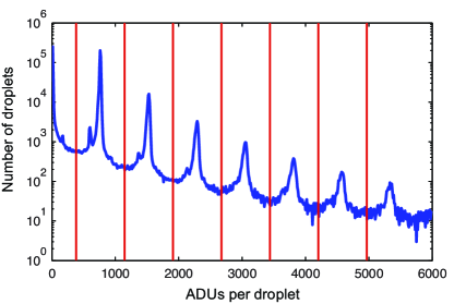
Figure 10: (Supplemental) Histogram of analog-to-digital units (ADU) per droplet, for all of the 309 images reported for liquid Ga. Integer photon peaks occur at multiples of 764 ADU, and Si K$\alpha$ escape peaks can be seen below the primary peaks. Vertical lines show boundaries used to separate droplets into integer numbers of photons.

d) The initial guess for photon positions in a droplet comes from the centers of the pixels assigned in step a), randomized by $\pm 0.5$ pixel in $x$ and $y$.

d) A weighted chi square representing the square of the deviation of the fit function from the data is calculated for each step in the fitting process, and the position parameters are varied until a minimum chi square is found.

e) The fitting procedure is run 4 times for each droplet, starting with a new randomization of the initial guess. The positions from the fit with the minimum final chi square are chosen.

f) These photon positions relative to the droplet are reintegrated onto the full CCD array based on the droplet position. Photon positions from the special cases in step 6) are included. The photon positions shown in Fig. 1(c) of the main paper were obtained in this way.

We found that this droplet algorithm worked efficiently for images with $\bar{k}$ up to about 0.2. Above this value of $\bar{k}$, the droplets began to grow much larger and contain many photons as the percolation limit was approached, greatly slowing the fitting process.

III.3 Calculation of $\langle\beta\rangle$

Because both the incident pulse energy and effective photon energy bandwidth of each LCLS pulse can be different GuttPRL2011 , we expect each speckle pattern to have different values of $\bar{k}$ and $\beta$. Our strategy for extracting accurate contrast values using many weak speckle patterns is thus to obtain relatively inaccurate $\beta$ values from each pattern and to average them to obtain a more accurate overall $\langle\beta\rangle$.

To obtain $\beta$ for a given pattern from the photon positions, we first chose a region of pixels with nearly constant $\bar{k}$ (e.g. along the top of the main amorphous scattering ring, as shown in Fig. 1(a) of the main paper). We used 300-, 600-, or 1100-pixel-wide regions for the $L=18,35~{}{\rm to}~{}37,~{}{\rm or}~{}142$ cm sample-to-detector distances, respectively. The length of the region was 1200 pixels in all cases, so that the total numbers of pixels in the regions were $n_{pix}=3.6,7.2,~{}{\rm or}~{}13.2\times 10^{5}$, respectively. These regions gave a variation of $\bar{k}$ of less than 5%.

To calculate $P(k)$, each pixel within the chosen region was assigned the number of photons that had positions anywhere within its borders. The experimental $P(k)$ for that image are given by the number of pixels with $k$ photons divided by $n_{pix}$. The experimental value of $\bar{k}$ for that image was obtained from the total number of photons divided by $n_{pix}$.

The method we used to obtain $\langle\beta\rangle$ from the $P(k)$ for a sequence of speckle patterns was to calculate the quantity $R\equiv 2P(2)[1-P(1)]/P(1)^{2}$ for each pattern and perform a weighted average to obtain a value of $\langle R\rangle$ for the set of patterns. The weighting was based on the experimental uncertainties in $R$ which are dominated by the relatively small number of $k=2$ pixels, as described above. Patterns with $\bar{k}>0.2$ were not included, because of errors introduced by the droplet algorithm. Patterns with $\bar{k}<(2/n_{pix})^{1/2}$ were not included, because below this limit the expected number of pixels with $k=2$ becomes less than one for $\beta=0$. The value of $\langle\beta\rangle$ was calculated from $\langle R\rangle$ by numerically inverting the exact negative binomial expression for $2P(2)[1-P(1)]/P(1)^{2}$ using the average value $\langle\bar{k}\rangle$ for the set of patterns. This corrects for the small deviation of $R$ from $1+\beta$ at higher $\bar{k}$ values. The RMS uncertainties in $\langle\beta\rangle$ reported in Table I of the main paper were obtained by carrying the experimental uncertainties through the weighted averaging procedure.

As can be seen from Fig. 2 in the main paper, this method for obtaining $\langle\beta\rangle$ from the values of $P(2)$ and $P(1)$ gives good agreement with the observed values of $P(3)$ and $P(4)$ for single-pulse measurements. Fitting of a single value of $\beta$ to all of the $P(k)$ values as a function of $\bar{k}$ gave an equivalent result for the single-pulse measurements.

However, we found that for the speckle patterns recorded using multiple LCLS pulses, the observed values of $P(k)$ for $k>2$ were typically higher than predicted by the $\langle\beta\rangle$ extracted from $P(2)$ and $P(1)$. This effect is consistent with the $P(k)$ predicted for the summation of speckle from individual pulses with varying values of $\beta$ because of variations in the effective x-ray photon energy bandwidth. Since the summation of patterns of different $\beta$ gives values of $P(1)$ and $P(2)$ that agree with the average $\langle\beta\rangle$ to first order, we chose to use the procedure outlined above to extract the contrast factors for all of the data.

IV Estimated Temperature Increase from X-ray Absorption

Because the sub-picosecond x-ray pulse width is much smaller than the time constant for thermal diffusion into the bulk from micron-scale volumes, the energy deposited by x-ray absorption can significantly heat the probed region of the sample when focused LCLS beams are used. This is a particular concern for XPCS measurements where we wish to study the equilibrium dynamics of the sample without perturbation by the x-ray probe.

For the Si (111) bandwidth monochromatic x-ray beam used here, we find that typical unattenuated single pulses focused to a $1.6\times 1.7~{}\mu$m FWHM spot melted or vaporized the illuminated region of Ga and Ni₂Pd₂P samples. Figures 11-12 (Suppl.) show scanning electron microscope (SEM) images of damage pits left in Ni₂Pd₂P glass by single LCLS pulses of different pulse energy. Major vaporization occurs for $I_{0}=2.4\times 10^{10}$ photons while only melting appears to have occurred for $3.3\times 10^{9}$ photons. Pulse energies of $2.1\times 10^{9}$ photons and below left no mark visible in SEM.

One can calculate the absorbed energy per atom in the illuminated volume as $4I_{0}E_{phot}/(\rho_{at}\ell_{abs}\pi s_{h}s_{v})$, where $E_{phot}$ is the photon energy, $\rho_{at}$ is the atomic density, $\ell_{abs}$ is the incident x-ray absorption length, and $s_{h}$ and $s_{v}$ are the transverse beam sizes. The observed maximum pulse energy $I_{0}=2.1\times 10^{9}$ that leaves no mark on the Ni₂Pd₂P sample corresponds to 13 eV per illuminated atom absorbed energy. Assuming a typical heat capacity of $3k_{B}=2.6\times 10^{-4}$ eV/K per atom one can estimate the adiabatic temperature rise that would occur if all of the absorbed energy remained in the illuminated volume. This simple calculation gives an adiabatic temperature rise of $5\times 10^{4}$ K.

The thermal energy density needed to leave a damage mark can be estimated by considering the time constant for viscous flow $\tau_{vf}$ relative to that for thermal diffusion $\tau_{th}$ calculated the measured properties of Ni₂Pd₂P. Using a thermal diffusivity $D_{th}=2.2\times 10^{-6}$ m²/s NPPdiffth , the thermal time constant for dissipation of the heat from the x-ray pulse into the bulk is $\tau_{th}=r^{2}/4D_{th}\approx 1~{}\mu$s for a length scale $r$ of a few microns. The time constant for viscous flow is Stephenson88 $\tau_{vf}=6\eta(1-\nu)/E$, where $\eta$ is the viscosity, $\nu$ is Poisson’s ratio, and $E$ is Young’s modulus, all of which have been measured for Ni₂Pd₂P glass NPPvisc ; NPPPois ; NPPYoung . For a damage mark to occur, $\tau_{vf}$ must be much less than $\tau_{th}$, which requires a temperature approaching 900 K to get into the low-viscosity liquid $\eta<10^{4}$ Pa-s NPPvisc . Taking into account the doubling of the heat capacity at temperatures above the glass transition at $\sim$550 K NPPheatcap , we estimate that a damage mark will occur at deposited thermal energy densities above about 0.26 eV per atom. Comparing this to the observed damage threshold fluence of 13 eV per illuminated atom, this indicates that the absorbed energy is thermalized in a volume about 50 times as large as the illuminated volume for these micron-scale incident beams.

Because the x-ray absorption process involves a cascade of photoelectrons, secondary electrons, fluorescent photons, and optical phonons that can propagate a significant distance before the absorbed energy is transferred to a thermal population of lattice vibrations Cargill , for small incident beams one indeed expects that the volume of material that is initially heated to be larger than the illuminated volume. The maximum temperature rise $\Delta T$ can be estimated as

$$\Delta T=\frac{I_{0}E_{phot}}{3k_{B}\rho_{at}\ell_{abs}\pi(s_{h}^{2}/4+r_{d}^{2})^{1/2}(s_{v}^{2}/4+r_{d}^{2})^{1/2}},$$ (9)

where $r_{d}$ is the effective diffusion length of the non-thermal electron-phonon cascade. For the beam size used here ($s_{h}=1.6~{}\mu$m, $s_{v}=1.7~{}\mu$m), a cascade diffusion length of $r_{d}\approx 6~{}\mu$m would agree with the observed factor of 50 larger volume in which the absorbed energy is thermalized. This is in rough agreement with the smallest melted regions observed, e.g. Fig. 12 (Suppl.), and with theoretical expectations, since typical values for photoelectron propagation Cargill and electron excitation depths Potts are in the few-micron range.

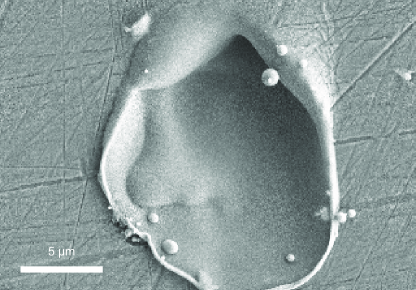
Figure 11: (Supplemental) Scanning electron micrograph of damage pit left by single pulse of monochromatic 7.99 keV x-rays from LCLS containing $2.4\times 10^{10}$ photons (31 $\mu$J) focused to a $1.6\times 1.7~{}\mu$m FWHM spot, incident at 15 degrees onto the surface of Ni₂Pd₂P metallic glass (scan 133 pulse 24). The fluence of 1100 J/cm² and absorption length of $8.2~{}\mu$m correspond to an average energy deposition of 150 eV per atom in the illuminated volume.

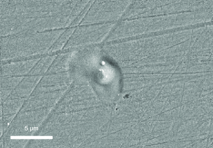
Figure 12: (Supplemental) Scanning electron micrograph of damage pit left by single pulse of monochromatic 7.99 keV x-rays from LCLS containing $3.3\times 10^{9}$ photons (4.2 $\mu$J) focused to a $1.6\times 1.7~{}\mu$m FWHM spot, incident at 15 degrees onto the surface of Ni₂Pd₂P metallic glass (scan 133 pulse 23). The fluence of 155 J/cm² and absorption length of $8.2~{}\mu$m correspond to an average energy deposition of 21 eV per atom in the illuminated volume.

For the liquid Ga sample, the vaporizations of the illuminated volume by intense single pulses were observed to cause recoils that changed the shape of the droplet, which then slowly returned to its original spherical shape. We did not observe any visible change in the B₂O₃ fibers even by the most intense pulses.

V Split-Pulse XPCS Feasibility

One measure of the x-ray fluence that can be tolerated can be obtained from our current measurements of the threshold of pulse energy that reduced the speckle contrast in multiple-pulse patterns from the glass samples. We estimate that the threshold to permanently perturb the sample structure corresponds to x-ray pulses of $I_{0}=1.6\times 10^{8}$ or $1.4\times 10^{10}$ photons of $E_{phot}=7.99$ keV for Ni₂Pd₂P or B₂O₃, respectively. These perturbation thresholds both correspond to an absorbed energy per illuminated atom of about 1 eV, or a maximum temperature rise of about 80 K from Eq. (9), owing to the different x-ray absorption lengths of Ni₂Pd₂P and B₂O₃. Pulses of this fluence caused no significant permanent rearrangement of the atomic-scale structure e.g. through atomic diffusion. However, when studying samples with more temperature-sensitive diffusion dynamics, or more sensitive processes such as phonon dynamics, an 80 K temperature rise may disturb the dynamics. Here we will estimate the minimum x-ray fluence and temperature rise needed to obtain sufficient signal-to-noise to perform XPCS measurements.

The figure of merit for split-pulse XPCS measurements developed above, $\beta/\sigma_{\beta}$, is the same as that previously developed for standard “sequential” XPCS measurements FalusJSR2006 ; LudwigJSR2011 , and the expression in terms of experimental parameters $\beta/\sigma_{\beta}=\beta\bar{k}[n_{pix}n_{patt}/2(1+\beta)]^{1/2}$ is very similar. Both have the same linear dependence on $\beta\bar{k}$ and square root dependence on $n_{pix}n_{patt}$. If sample perturbation by the x-ray beam is not an issue, then a strategy to maximize the figure of merit is to increase the mean photon density $\bar{k}$ at fixed $\beta$ by decreasing the focal spot size and increasing the angle $p/L$ subtended by each pixel, even if the available solid angle is limited and the number of pixels $n_{pix}$ must thus decrease.

The mean photon density on the detector for a single pulse can be extrapolated from our measured values using the expression

$$\bar{k}=\Sigma_{v}I_{0}t\left(\frac{p}{L}\right)^{2},$$ (10)

where $\Sigma_{v}$ is a sample-dependent cross section per unit volume. By averaging the $\Sigma_{v}$ values obtained from our measured values of $\bar{k}$ per pulse for each type of sample, we obtain $\Sigma_{v}\approx 42$, 100, and 1.3 m^-1 rad^-2 for Ga, Ni₂Pd₂P and B₂O₃, respectively.

In the limit of large detector pixel subtended angle $p/L$, the expressions given above for $\beta_{calc}$ reduce to $\beta=\lambda^{2}(p/L)^{-2}s_{h}^{-1}(s_{v}^{2}\cos^{2}2\theta+t^{2}\sin^{2}2\theta)^{-1/2}$, where $\beta$ is much smaller than unity. Thus $\beta\bar{k}$ becomes independent of $p/L$, and is given by

$$\beta\bar{k}=\frac{\lambda^{2}\Sigma_{v}I_{0}t}{s_{h}(s_{v}^{2}\cos^{2}2\theta+t^{2}\sin^{2}2\theta)^{1/2}}.$$ (11)

In this limit the signal to noise ratio $\beta/\sigma_{\beta}=\beta\bar{k}[n_{pix}n_{patt}/2(1+\beta)]^{1/2}$ is given by

$$\frac{\beta}{\sigma_{\beta}}=\frac{\lambda^{2}\Sigma_{v}I_{0}t}{s_{h}}\left(\frac{n_{pix}n_{patt}}{2s_{v}^{2}\cos^{2}2\theta+2t^{2}\sin^{2}2\theta}\right)^{1/2}.$$ (12)

To estimate the signal-to-noise ratio for an optimized XPCS experiment at LCLS, we choose an incident x-ray pulse energy $I_{0}$ to produce a given temperature rise $\Delta T$ for a given beam size $s=s_{v}=s_{h}$ and sample according to Eq. (9), giving

$$\frac{\beta}{\sigma_{\beta}}=\frac{3k_{B}\Delta T\lambda^{2}\Sigma_{v}t\rho_{at}\ell_{abs}\pi(n_{pix}n_{patt})^{1/2}(s^{2}/4+r_{d}^{2})}{E_{phot}s(2s^{2}\cos^{2}2\theta+2t^{2}\sin^{2}2\theta)^{1/2}}.$$ (13)

Values of $Q\equiv 4\pi\sin\theta/\lambda$ and $t$ from Table I (Suppl.) are used, except $t=200~{}\mu$m for B₂O₃. We assume a detector capable of recording $n_{pix}=10^{6}$ pixels at the full LCLS repetition rate of 120 Hz, to give $n_{patt}=4\times 10^{4}$ in six minutes per delay time. Figure 13 (Suppl.) shows the signal-to-noise ratio as a function of beam size $s$ for a fixed $\Delta T=10$ K, for each of the three samples. The solid curves correspond to the expected cascade diffusion length of $r_{d}\approx 6~{}\mu$m, and show that the best signal to noise is obtained with small beam sizes. This suggests that adequate signal-to-noise values (above the value of 5 shown by the dashed black line) can be obtained for all samples in this regime. At beam sizes smaller than $r_{d}$, the $I_{0}$ to give $\Delta T=10$ K from Eq. (9) becomes independent of beam size and is given by $I_{0}=18,0.5,~{}{\rm or}~{}0.2\times 10^{8}$ photons per pulse for B₂O₃, Ga, or Ni₂Pd₂P, respectively. Such pulse energies are expected to be available even when using the narrow energy bandwidth of $\Delta E/E=10^{-5}$ from the pulse split-and-delay RosOE2009 ; RosJSR2011 .

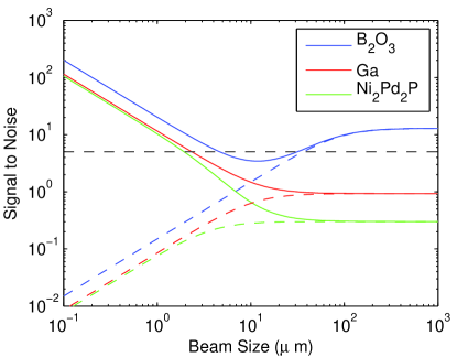
Figure 13: (Supplemental) Estimated optimized signal-to-noise ratio as a function of beam size for the three samples (Ga, Ni₂Pd₂P, and B₂O₃), with pulse energy $I_{0}$ set to give a temperature rise of $\Delta T=10$ K. Solid curves are for a cascade diffusion length of $r_{d}=6~{}\mu$m, while dashed curves show the behavior for $r_{d}=0$. Black dashed line shows minimum required signal-to-noise ratio of 5.

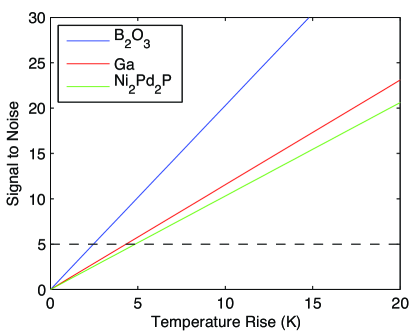
Figure 14: (Supplemental) Estimated optimized signal-to-noise ratio as a function of temperature rise for the three samples (Ga, Ni₂Pd₂P, and B₂O₃), using a beam size $s=1~{}\mu$m, for $r_{d}=6~{}\mu$m. Black dashed line shows minimum required signal-to-noise ratio of 5.

The dashed curves on Fig. 13 (Suppl.) show the estimated behavior expected for the case of $r_{d}=0$, where all absorbed energy is thermalized within the illuminated volume. In this limit, the best signal to noise is obtained for large beam sizes. Adequate signal-to-noise values are still expected for samples with low absorption such as B₂O₃.

Figure 14 (Suppl.) shows the signal-to-noise ratios as a function of temperature rise for a fixed beam size of $s=1~{}\mu$m, for $r_{d}=6~{}\mu$m. The signal-to-noise ratio and temperature rise both scale linearly with $I_{0}$. The estimated temperature rise needed to give a signal-to-noise ratio of 5 is $\Delta T=3.3,6.0,~{}{\rm or}~{}6.5$ K, and the pulse energy is estimated to be $I_{0}=6,0.3,~{}{\rm or}~{}0.13\times 10^{8}$ photons per pulse, for B₂O₃, Ga, or Ni₂Pd₂P, respectively. These temperature rises are significantly below the 80 K threshold for permanent structural disturbance that we observed for the glass samples, indicating that even more sensitive samples and processes can be studied. By using beam sizes smaller than $1~{}\mu$m, it may be possible to reduce $\Delta T$ even further. However, ultrafast processes that disturb the sample structure on time scales shorter than that for thermalization of the absorbed energy may become the limiting factor for very small beam sizes, as described below.

VI Sample Disturbance During Single Pulses

We observed that the average contrast factor $\langle\beta\rangle$ for single pulses was typically somewhat smaller than that calculated for a static sample, $\beta_{calc}$, indicating that there could be some motion of the atoms on the time scale of the x-ray pulse. The ratio $\langle\beta\rangle/\beta_{calc}$ was smaller for Ni₂Pd₂P than for Ga, and the average energy deposited per atom per pulse was larger, consistent with motion driven by the energy of the x-ray pulse. To evaluate the threshold above which the atomic structure could be disturbed during the time scale of the pulse, in Fig. 15 (Suppl.) we have plotted the ratio $\beta/\beta_{calc}$ vs. energy density deposited in the illuminated volume for each individual pulse in the sequences for Ni₂Pd₂P and Ga taken with $L=35$ cm. While the uncertainties of the individual points are relatively large, there is a clear trend toward lower contrast for higher deposited energy densities. Energy densities above about 50 eV per atom reduce the single-pulse speckle contrast. This illustrates the ability of speckle contrast to reflect atomic-scale, sub-picosecond dynamics, and indicates that x-ray fluences corresponding to absorbed energy densities above 50 eV per atom are likely to affect experiments in which single-pulse speckle patterns are analyzed to obtain atomic-scale structural information, for x-ray pulses corresponding to 70 fs electron pulse widths.

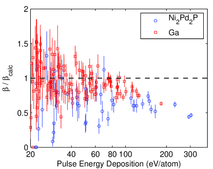
Figure 15: (Supplemental) Ratio of extracted contrast factor $\beta$ to the calculated value $\beta_{calc}$ for single-pulse speckle patterns as a function of the x-ray pulse energy expressed as energy deposited per atom in the illuminated volume. Data shown are from the sequences of single-pulse speckle patterns taken with L = 35 and 37 cm for Ga and Ni₂Pd₂P, respectively.

While the damage-mark threshold measurements described and modeled above indicate that the energy absorbed in the illuminated volume can be thermalized in a much larger volume for micron-scale beams, thus reducing the sample disturbance, ultrafast processes occurring prior to thermalization can lead to a more restrictive intensity threshold for sample disturbance for very small beams. For example, for the $I_{0}$ values used in Fig. 13 (Suppl.) which produce $\Delta T=10$ K according to Eq. (9), the threshold of 50 eV per illuminated atom which we observe to disturb the structure during the x-ray pulse will be exceeded for beam sizes smaller than $s=0.08~{}\mu$m.

VII Acknowledgement

Special thanks go to T. Hufnagel for the use of his metallic glass laboratory and to A. Zholents for insightful comments. X-ray experiments were carried out at LCLS at SLAC National Accelerator Laboratory, an Office of Science User Facility operated for the U.S. Department of Energy (DOE) Office of Science by Stanford University. Work at Argonne National Laboratory supported by the DOE Office of Basic Energy Sciences under contract DE-AC02-06CH11357. Electron microscopy was accomplished at the Electron Microscopy Center for Materials Research at Argonne, a DOE Office of Science User Facility.

References

- (1) J. W. Goodman, Speckle Phenomena in Optics : Theory and Applications (Roberts & Co., Englewood, Colo., 2007).
- (2) C. Gutt et al., Phys. Rev. Lett. 108, 024801 (2012).
- (3) L. Young et al., Nature 466, 56 (2010).
- (4) S. Duesterer et al., New Journal of Physics 13, 093024 (2011).
- (5) G. B. Stephenson et al. in LCLS: The First Experiments (2000), www-ssrl.slac.stanford.edu/lcls/papers/lcls_experiments_2.pdf.
- (6) G. Grübel, G. B. Stephenson, C. Gutt, H. Sinn, and T. Tschentscher, Nucl. Instrum. Meth. B 262, 357 (2007).
- (7) C. Gutt et al., Optics Express 17, 55 (2009).
- (8) P. N. Pusey, Statistical properties of scattered radiation, in Photon Correlation Spectroscopy and Velocimetry, edited by H. Z. Cummings and E. R. Pike, pages 45–141, Plenum, New York, 1974.
- (9) M. Sutton, Coherent x-ray diffraction, in Third-Generation Hard X-ray Synchrotron Radiation Sources: Source Properties, Optics, and Experimental Techniques, edited by D. M. Mills, John Wiley and Sons Inc., New York, 2002.
- (10) K. Ludwig, J. Synchr. Rad. 19, 66 (2012).
- (11) F. Livet, Acta Cryst. A 63, 87 (2007).
- (12) F. Livet et al., Nucl. Instrum. Meth. A 451, 596 (2000).
- (13) P. Falus, L. Lurio, and S. Mochrie, J. Synchr. Rad. 13, 253 (2006).
- (14) U. Harms, T.D. Shen, R.B. Schwarz, Scripta Mater. 47, 411 (2007).
- (15) G. B. Stephenson, Acta Metall. 36, 2663 (1988).
- (16) K. H. Tsang, S. K. Lee, and H. W. Kui, J. Appl. Phys. 70, 4837 (1991).
- (17) V. N. Novikov and A. P. Sokolov, Phys. Rev. B 74, 064203 (2006).
- (18) W. J. Wright, R. B. Schwarz, and W. D. Nix, Mater. Sci. Eng. A319-321, 229 (2001).
- (19) G. Wilde, G. P. G rler, R. Willnecker, and G. Dietz, Appl. Phys. Lett. 65, 397 (1994)
- (20) A. Erbil, G. S. Cargill, R. Frahm, and R. F. Boehme, Phys. Rev. B 37, 2450 (1988).
- (21) P. J. Potts, Handbook of Silicate Rock Analysis, (Blackie, London, 1987), p. 336.
- (22) W. Roseker et al., Optics Lett. 34, 1768 (2009).
- (23) W. Roseker et al., J. Synchr. Rad. 18, 481 (2011).