NLTE line formation of Fe for late-type stars. I. Standard stars with 1D and $\langle 3\rm{D}\rangle$ model atmospheres

Abstract

We investigate departures from LTE in the line formation of Fe for a number of well-studied late-type stars in different evolutionary stages. A new model of Fe atom was constructed from the most up-to-date theoretical and experimental atomic data available so far. Non-local thermodynamic equilibrium (NLTE) line formation calculations for Fe were performed using 1D hydrostatic MARCS and MAFAGS-OS model atmospheres, as well as the spatial and temporal average stratifications from full 3D hydrodynamical simulations of stellar convection computed using the Stagger code. It is shown that the Fe I/Fe II ionization balance can be well established with the 1D and mean 3D models under NLTE including calibrated inelastic collisions with H I calculated from the Drawin’s (1969) formulae. Strong low-excitation Fe I lines are very sensitive to the atmospheric structure; classical 1D models fail to provide consistent excitation balance, particularly so for cool metal-poor stars. A better agreement between Fe I lines spanning a range of excitation potentials is obtained with the mean 3D models. Mean NLTE metallicities determined for the standard stars using the 1D and mean 3D models are fully consistent. Also, the NLTE spectroscopic effective temperatures and gravities from ionization balance agree with that determined by other methods, e.g., infrared flux method and parallaxes, if one of the stellar parameters is constrained independently.

1 Introduction

Accurate determination of basic stellar parameters is fundamental for calculations of chemical composition, ages, and evolutionary stages of stars. One of the most commonly used methods to determine effective temperature $T_{\mathrm{eff}}$, surface gravity $\log g$ and metallicity [Fe/H], is to exploit excitation-ionization equilibria of various chemical elements in stellar atmospheres. Iron, with its partly filled $3d$ subshell, has, by far, the largest number of lines all over the spectrum of a typical late-type star. This atomic property coupled to a relatively large abundance makes it a reference element for spectroscopic estimates of stellar parameters.

The goal of this work is to study systematic uncertainties in this method, which are related to 1) the assumption of local thermodynamic equilibrium (LTE) in spectral line formation calculations, and 2) the use of theoretical 1D hydrostatic model atmospheres. These two approximations are inherent in most of the line formation codes utilized in spectroscopic studies, since they strongly reduce the complexity of the problem permitting the analysis of very large stellar samples in short timescales. Yet, in conditions when the breakdown of LTE/1D modelling occurs the inferred stellar parameters may suffer from large systematic biases (e.g., Asplund 2005). To assess the extent of the latter, more physically realistic modeling is necessary.

Non-local thermodynamic equilibrium (NLTE) effects on the Fe i/Fe ii level populations for FGK stars have been extensively discussed in the literature (Athay & Lites 1972; Cram, Lites & Rutten 1980; Bikmaev, Bobritskii & Sakhibullin 1990; Thévenin & Idiart 1999; Gehren et al. 2001; Gehren, Korn & Shi 2001; Collet et al. 2005; Mashonkina et al. 2011). These and other studies showed that NLTE effects in the ionization balance of Fe i/Fe ii are large for giants and metal-poor stars. The effect on solar-metallicity stars is smaller, but it is must be taken into account if one aims at the accuracy of few percent, as is the case for the Sun. Despite major efforts aimed at understanding how non-equilibrium thermodynamics affects the line formation of Fe, there have been only few attempts to quantify these deviations in a systematic manner across the Hertzsprung-Russell diagram. Mashonkina (2011) provided a small grid of NLTE corrections to five Fe i lines for the solar-metallicity stars with $T_{\mathrm{eff}}>6500$ K and $\log g>3$. Thévenin & Idiart (1999) explored a larger range of stellar parameters including FGK stars down to [Fe/H] $\approx-3$, however, they did not present a regular grid of NLTE corrections.

Furthermore, it has only recently become possible to perform full time-dependent, 3D, hydrodynamical simulations of radiative and convective energy transport in stellar atmospheres. Such simulations (Nordlund & Drawins 1990, Asplund et al. 1999, Collet et al. 2006, Ludwig et al. 2006, Nordlund, Stein & Asplund 2009, Freytag et al. 2010) have evidenced important shortcomings of 1D, stationary, hydrostatic models. Especially at low metallicity, it has been realized that 1D models, by necessarily enforcing radiative equilibrium, overestimate the average temperatures of shallow atmospheric layers, with profound implications for the spectral line formation (Collet, Asplund & Trampedach 2007, e.g., ).

In this work, we perform NLTE line formation calculations for Fe i and Fe ii using 1D hydrostatic and mean 3D model atmospheres obtained from temporal and spatial averaging of 3D hydrodynamical simulations (hereafter, $\langle 3\rm{D}\rangle$). A new model of Fe atom is constructed from the most up-to-date theoretical and experimental atomic data available so far. Non-local thermodynamic equilibrium Fe abundances, effective temperatures, and surface gravities are derived for the Sun, Procyon, and four metal-poor stars. The efficiency of thermalization caused by inelastic H i collisions is calibrated as to satisfy ionization equilibrium by scaling the classical Drawin (1968, 1969) formulae. In the next paper in the series (Lind, Bergemann & Asplund, 2012, hereafter Paper II), we discuss NLTE effects on Fe i and Fe ii over a wide range of stellar parameters. That paper also presents a large grid of 1D NLTE abundance corrections for a wealth of lines in metal-rich and metal-poor dwarf and giant spectra.

Before proceeding with the description of the methods, we shall point out a few important aspects of our study. First, due to a comparative nature of the analysis (1D LTE vs. 1D NLTE and $\langle 3\rm{D}\rangle$ NLTE) no attempt is made to fine-tune various parameters in order to achieve full agreement with other results in the literature. Second, although by the use of the averaged 3D models we roughly account for hydrodynamic cooling associated with convective overshoot in the simulations, the effect of horizontal inhomogeneities is not addressed because such calculations with our new realistic extensive model atom are beyond current computational capabilities. We note, however, that our results are expected to closely resemble any future full 3D NLTE calculations once these become feasible. The reason is that in NLTE the Fe i line formation is largely dictated by the radiation field (as explained in detail below) originating in deep atmospheric layers, where the significance of the atmospheric inhomogeneities is greatly reduced. Detailed tests of the $\langle 3\rm{D}\rangle$ models, which involve comparison with other observable quantities, will be presented elsewhere (Collet et al., in prep.). Full 3D NLTE calculations with a simpler model atom of Fe will be a subject of a forthcoming publication.

The paper is structured as follows. Section 2 gives a brief description of the input model atmospheres, model atom, and programs used to compute NLTE populations and line formation. The results of statistical equilibrium calculations are presented in Sec. 3. The analysis of the solar spectrum along with the re-determination of the Fe abundances for the Sun and Procyon is described in detail in Sec. 4. Section 4.5 presents and discusses metallicities, temperatures, and gravities obtained for the metal-poor stars. Finally, a comparison with stellar evolution calculations is given in Sec. 4.6. A short summary of the work and conclusions are given in Sec. 5.

2 Methods

Figure 1: Comparison of the temperature and gas pressure structures in the marcs and $\langle 3\rm{D}\rangle$ model atmospheres. Arrows indicate the optical depths, above which the marcs models were extrapolated.

2.1 Model atmospheres

In the present study, we employ both mafags-os (Grupp 2004a, Grupp 2004b, Grupp, Kurucz & Tan 2009) and marcs (Gustafsson, Edvardsson, Eriksson, Jørgensen, Nordlund & Plez, 2008) 1D LTE hydrostatic model atmospheres, as well as 3D hydrodynamical models computed with the Stagger code (Galsgaard & Nordlund 1995, Collet et al. 2011).

The mafags-os models for all investigated stars were kindly provided by F. Grupp. The models are plane-parallel with convective energy transport based on the turbulent convection model of Canuto & Mazzitelli (1991). Compressible turbulence is accounted for using a mixing length, $\alpha_{\rm cm}=l/\rm{H_{p}}$$=0.82$. The reasons for this choice are discussed in Bernkopf (1998). We note that this $\alpha_{\rm cm}$ is also consistent with the results of Freytag, Ludwig & Steffen (1999), who attempted to calibrate the mixing length parameter using the 2D radiation hydrodynamics simulations of stellar convection. Line absorption is computed by the method of opacity sampling including $\sim 86\,000$ wavelength points from extreme UV to far IR. Extensive line lists were extracted from Kurucz and VALD databases. The reference solar abundances were compiled from various literature sources, giving preference to NLTE determinations by the Munich group (e.g., Gehren et al., 2001). In particular, the solar Fe abundance is set to $\log\varepsilon_{\odot}=7.50$.

The marcs models are based on opacity sampling with $\sim 10^{4}-10^{5}$ wavelength points using Kurucz and VALD linelists. Convection is included in the Henyey, Vardya & Bodenheimer (1965) version of the mixing length theory with the mixing length parameter set to $\alpha_{\rm MLT}=1.5$. A detailed description of the models can be found on the MARCS web-site. For the majority of the elements, the reference solar abundances are that of Asplund et al. (2005).

Three-dimensional radiation-hydrodynamic simulations of convection at the surface of the Sun and reference stars were computed using the Copenhagen Stagger code (Nordlund & Galsgaard 1995). The physical domains of the simulations cover a representative portion of the stellar surface. They include the whole photosphere as well as the upper part of the convective layers, typically encompassing $12$ to $15$ pressure scale heights vertically. Horizontally, they extend over an area sufficiently large to host about ten granules at the surface. The simulations use realistic input physics, including state-of-the-art equation-of-state, opacities, and treatment of non-grey radiative transfer. The adopted reference solar chemical composition for the simulations is that of Asplund, Grevesse, Sauval & Scott (2009). For a more detailed description of the simulations’ setup, we refer to Collet, Magic & Asplund (2011).

For the purpose of the current study, we computed spatial and temporal averages of these simulations over surfaces of equal optical depth $\log\tau_{\rm 5000}$ at the chosen reference wavelength at $5000$ Å. The independent thermodynamic variables, gas density $\rho$ and internal energy per unit mass $\varepsilon$, as well as the temperature $T$ are first interpolated with cubic splines for all columns in the full 3D structure to the reference optical depth scale. The reference scale was constructed to cover the relevant range for line-formation calculations (${-5}{\la}~{}{\log\tau_{\rm 5000}}~{}{\la}{2}$) evenly in $\log\tau_{\rm 5000}$. For density and internal energy, a logarithmic interpolation is used. Other physical quantities, namely gas pressure $P_{\rm gas}$ and electron number density $n_{\rm el}$, are looked up from the simulations’ equation-of-state tables as a function of density and internal energy. Finally, mean $\langle 3\rm{D}\rangle$ stratifications are constructed by averaging the various physical quantities pertinent to line-formation calculations, $\ln{\rho}$, $T$, $\ln{P_{\rm gas}}$, and $\ln{n_{\rm el}}$, on surfaces of equal optical depth $\log\tau_{\rm 5000}$ and over time (i.e., over all simulation snapshots). We emphasize that no hydrostatic equilibrium was enforced after the averaging process. In the present application of mean $\langle 3\rm{D}\rangle$ stratifications to line-formation calculations, averages of velocity fields were not considered, and line broadening associated with bulk gas flows and turbulence was accounted for by means of a classical, depth-independent micro-turbulence parameter (Sect. 2) as in 1D models.

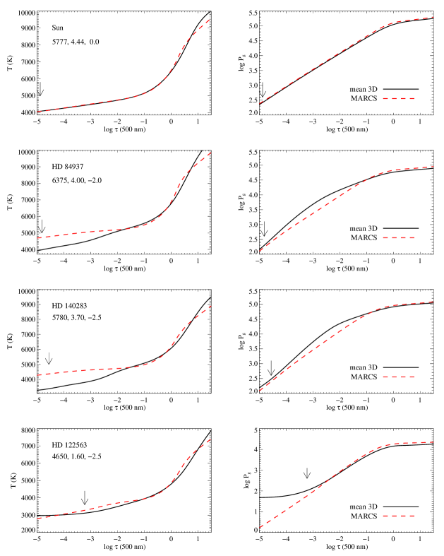
The temperature and pressure stratifications from the 1D marcs model atmospheres and the mean $\langle 3\rm{D}\rangle$ hydrodynamical models of the Sun and three metal-poor standard stars are shown in Fig. 1 as a function of continuum optical depth at $5000$ Å.The input parameters are the ones listed in Table 1. The mafags-os models are not included in the plots, because they adopt slightly different stellar parameters. Due to the similar equation-of-state, marcs and mafags-os model atmospheres are essentially identical in the outer layers. The differences between 1D and $\langle 3\rm{D}\rangle$ models are more pronounced, especially in the case of metal-poor stellar atmospheres. At low metallicities, 3D stellar surface convection simulations predict cooler upper photospheric stratifications (Asplund, Nordlund, Trampedach & Stein 1999, Collet, Asplund & Trampedach 2007), than corresponding classical, hydrostatic, stationary 1D model atmospheres generated for the same stellar parameters. The temperature in the outer layers of time-dependent, 3D, hydrodynamical simulations is mainly regulated by two mechanisms: radiative heating due to reabsorption of continuum radiation by spectral lines and adiabatic cooling associated with expanding gas above granules. At low metallicities, the coupling between radiation and matter is weakened with respect to the solar-metallicity case because of the decreased line opacities; the adiabatic cooling term therefore prevails, causing the thermal balance to shift toward on average lower temperatures. Stationary, 1D, hydrostatic models do not account for this cooling term associated with diverging gas flows, and the thermal balance in the upper photosphere is controlled by radiative heating and cooling only, ultimately leading, at low metallicities, to higher equilibrium temperatures than predicted by 3D models (Fig. 1, left panels). The lower average temperatures in the outer layers of metal-poor 3D models also imply smaller values of the pressure scale height and, consequently, steeper pressure stratifications on a geometrical scale with respect to corresponding 1D models. However, the lower temperatures also result in lower opacities; therefore, on an optical depth scale, the average gas pressure in the optically thin layers of the metal-poor 3D models appears typically higher at a given optical depth than in 1D models (Fig. 1, right panels).

2.2 Statistical equilibrium codes

The NLTE level populations of Fe i and Fe ii were computed with an updated version of the detail code (Butler & Giddings, 1985) and multi (Carlsson, 1986, 1992). In both codes, the solution of the coupled statistical equilibrium and radiative transfer equations is obtained using an approximate lambda iteration method. In detail, the latter is implemented following a $\Psi$-operator approach of the kind described by Rybicki & Hummer (1991, 1992), which allows for self-consistent treatment of overlapping transitions and continua. multi is based on the method described by Scharmer & Carlsson (1985) with the local operator by Olson, Auer & Buchler (1986). Scattering in the bound-bound (hereafter, b-b) transitions included in the model atom follows complete frequency redistribution. Upper boundary conditions differ in that detail assumes no incoming radiation at the top, whereas multi estimates the minor contribution from the optically thin gas and uses a second order Taylor expansion of the Feautrier variables. Ng convergence acceleration (Ng, 1974; Auer, 1987) is implemented in both codes.

In both codes, the background line opacity is computed with a Planckian source function. However, there is one difference. In detail, line opacity is consistently added at the frequencies of all b-b and b-f transitions in the NLTE atom. In multi, metal line opacities were added to the continuous opacities for the calculation of photoionization rates only, as described by Collet et al. (2005), while blends were neglected in the calculation of the bound-bound radiative rates. This approximation is well justified and saves computational time. Firstly, Fe itself dominates line opacity in the UV. Secondly, according to our tests, the upper limit to the differences in the NLTE equivalent widths computed with and without blends is $\sim 0.2$ percent for the Sun and $5$ percent for HD 122563.

When solving for statistical equilibrium, Fe line profiles were computed with a Gaussian in detail and with Voigt profiles in multi. Although the latter is also possible with detail, it is un-necessary. Our tests showed that NLTE effects in Fe i are insensitive to the adopted profile functions. Once the level populations were converged with detail, the synthetic line profiles were computed with SIU (Reetz, 1999).

Finally, we remark on the handling of the equation-of-state in the NLTE codes. Whereas multi includes a subroutine to compute ionization fractions and molecular equilibria internally, detail and siu require partial pressures of all atoms and important molecules to be supplied with a model atmosphere. These are included in the mafags-os models. For the marcs and $\langle 3\rm{D}\rangle$ models, we computed the atomic partial pressures using the equation-of-state package built in multi.

2.3 Model atom of Fe

2.3.1 Levels and radiative transitions

Figure 2: Grotrian diagram of the Fe ii (top) and Fe i atoms (bottom). Predicted levels are shown in red. Only lines selected for the abundances analysis are shown.

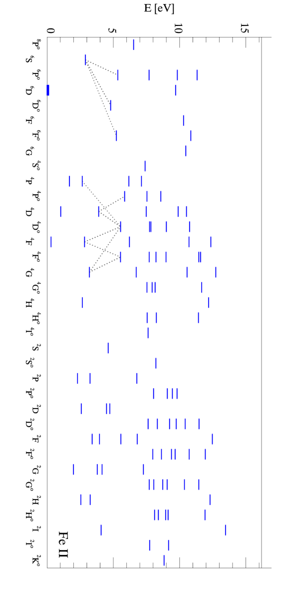
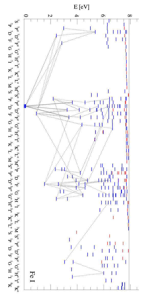
The number of levels and discrete radiative transitions in Fe is enormous. Recent calculations of Kurucz predict $\sim 37\,000$ theoretical energy levels below and above the first ionization threshold of Fe i, as well as $6\,025\,000$ radiatively-permitted transitions between them. Such atomic models are not tractable with our NLTE codes; thus, we combined atomic levels and transitions into super-levels and super-lines (see below). In our final model, which also includes all experimental data from the NIST atomic database (Ralchenko et al., 2012), the number of energy levels is $296$ for Fe i and $112$ for Fe ii, with uppermost excited levels located at $0.03$ eV and $2.72$ eV below the respective ionization limits, $7.9$ eV and $16.19$ eV. The model is closed by the Fe iii ground state. The total number of radiatively-allowed transitions is $16\,207$ ($13\,888$ Fe i and $2\,316$ Fe ii). Fine structure was neglected for all levels, but the ground states of Fe i $a\,^{5}{\rm D}$ (configuration $1s^{2}2s^{2}2p^{6}3s^{2}3p^{6}3d^{6}4s^{2}$) and Fe ii $a\,^{6}{\rm D}$. Excitation energy of each LS term is a weighted mean of statistical weights and excitation energies of fine structure levels. The mean wavelength for a multiplet is computed from the weighted energy levels.

All predicted energy levels of Fe i with the same parity above $E_{\rm low}\geq 5.1$ eV were grouped into superlevels. For the upper levels above $54000$ cm${}^{-}1$ ($6.7$ eV), we combined all levels within $1000$ cm^-1 ($0.12$ eV), whereas below this energy limit only levels deviating by less than $10$ cm^-1 ($0.001$ eV) were combined. Thus, not only predicted, but also some experimental levels above $5.1$ eV were combined to superlevels. None of the Fe lines selected for the subsequent abundance analysis has either the lower or the upper level combined.

Transitions between the components of the superlevels were also grouped preserving the parity and angular momentum conservation rules. The total transition probability of a superline is a weighted average of $\log gf$’s of individual transitions, and is computed in analogy to a $gf$-value for a multiplet (Martin, Fuhr & Wiese, 1988):

$$f_{\rm mean}=\frac{1}{\bar{\lambda}_{\rm mean}\sum_{l}g_{l}}\sum_{l,u}g_{l}\times\lambda_{\rm lu}\times f_{\rm lu}$$ (1)

where $l$ and $u$ are indices of lower and upper levels of the un-grouped transition, $\bar{\lambda}_{\rm mean}$ is the mean Ritz wavelength of a superline. Grotrian diagram of the Fe model atom is shown in Fig. 2. Although the accuracy of individual $gf$-values for the multitude of theoretically-computed transitions is hard to quantify, we expect our model to be a good representation of the global atomic properties of the Fe i/Fe ii and provide physically valid description of statistical equilibrium of the atom in the atmospheres of late-type stars.

Accurate radiative bound-free cross-sections for Fe i computed using the close-coupling method were kindly provided by M. Bautista (private communication 2011, Bautista 1997, see also). These data are computed on a more accurate energy mesh and provide better resolution of photoionization resonances compared to the older data, e.g. provided in the TOPbase. Thus, $136$ levels of Fe i, including different multiplet systems, from singlets to septets, are represented by quantum-mechanical data. Hydrogenic approximation was used for the other levels.

2.3.2 Collisional transitions

The rates of transitions induced by inelastic collisions with free electrons (e^-) and H i atoms were computed using different recipes. For states coupled by allowed b-b and b-f transitions, we used the formulas of van Regemorter (1962) and Seaton (1962), respectively, in the case of e^- collisions and that of Steenbock & Holweger (1984), in the case of H i collisions. Also, all states are coupled by forbidden transitions induced by $e^{-}$ collisions using the formula of Allen (1973) and by H i collisions with the formula of Takeda (1994).

We constrain the efficiency of collisions with H i empirically (Sect. 4, 4.5). We apply a scaling factor $S\!_{\rm H}$ to the cross-sections, which is iteratively derived from the constraint of Fe i/Fe ii ionization equilibrium for the standard stars with independently-fixed stellar parameters. As pointed out by Barklem et al. (2011), such approach is an over-simplification of the problem. However, at present there are no useful alternatives to this classical recipe. Evidence for the necessity of including inelastic collisions with H i in statistical equilibrium calculations for Fe and other elements has been demonstrated in many studies (e.g., Mashonkina et al., 2011), which is also confirmed by us (Sect. 4, 4.5).

3 Statistical equilibrium of Fe

In the following section, we present the results of statistical equilibrium calculations for Fe obtained with detail and multi. We briefly describe the physical processes responsible for deviations from LTE level populations in the Fe i and Fe ii atoms for atmospheric conditions typical of FGK stars. A comprehensive description of NLTE effects as a function of stellar parameters is deferred to the second paper of this series (Lind et al., 2012). The main aim here is to understand the differences in terms of NLTE Fe i line formation with 1D and $\langle 3\rm{D}\rangle$ model atmospheres, which is necessary in order to explain the large differences between the spectroscopic values of $T_{\mathrm{eff}}$, $\log g$, and [Fe/H] obtained for the reference stars in the two cases (Sect. 4.5).

Fe i is a minority ion in the atmospheres of late-type stars, which increases its sensitivity to NLTE over-ionization. The overall effect is that, compared to LTE, the statistical equilibrium of Fe favors lower number densities of the neutral ion, Fe i, although the number densities of relevant Fe ii levels remain nearly thermalized. In general, this leads to a weakening of Fe i lines compared to LTE that, in turn, requires larger Fe abundance to fit a given observed spectral line. The actual magnitude of departures and NLTE abundance corrections depends on stellar parameters (Sect. 4.5).

Figure 3: Departure coefficients for the four reference stars computed with the 1D marcs (left panel) and $\langle 3\rm{D}\rangle$ (right panel) model atmospheres.

Figure 3 presents the departure coefficients of selected Fe i and Fe ii levels computed for the marcs and $\langle 3\rm{D}\rangle$ model atmospheres with multi. The results are shown for the Sun, the metal-poor subdwarf HD 84937, the metal-poor sub-giant HD 140283 and the metal-poor giant HD 122563. Only a few, selected levels, typical for the dependence of their associated departure coefficients with depth, are included in the plot: $a\,^{5}{\rm D}_{\rm 4}$ (ground state of Fe i), $z\,^{7}{\rm D}^{{\rm\circ}}$ ($2.4$ eV), $e\,^{5}{\rm D}$ ($5.4$ eV), $t\,^{3}{\rm H}_{\rm\circ}$, and two levels, which belong to the Fe ii ion: $a\,^{6}{\rm D}_{\rm 9/2}$ (ground state) and $z\,^{4}{\rm D}^{{\rm\circ}}$ ($5.5$ eV). In the optically thin atmospheric layers these and majority of other Fe i levels are underpopulated compared to LTE, $b_{i}<1$. For all stars, but HD 122563, the Fe ii number densities remain close to LTE values throughout the atmosphere, $b_{i}\approx 1$, and a minor overpopulation of the Fe ii ground state develops only close to the outer atmospheric boundary.

Figure 4: Net bound-free radiative brackets computed for the solar marcs model atmosphere (top and middle panel). Optical depth is indicated in each panel. Red and blue dots indicate over-ionization and over-recombination, respectively.

Deviations from LTE in the distribution of atomic level populations arise because the mean radiation field, $J_{\nu}$, at different depths and frequencies is not equal to the Planck function, $B_{\nu}[T_{\rm e}(\tau)]$. For Fe i, excess of the mean intensity over Planck function in the UV continua leads to over-ionization, which sets in at $\log\tau_{\rm 5000}\approx 0.2$, i.e., as soon as the optical depth in the photoionization continuum of low-excitation Fe i levels with $E\approx 2$ eV falls below unity (Fig. 3a).

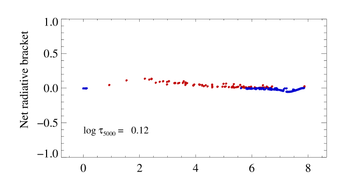
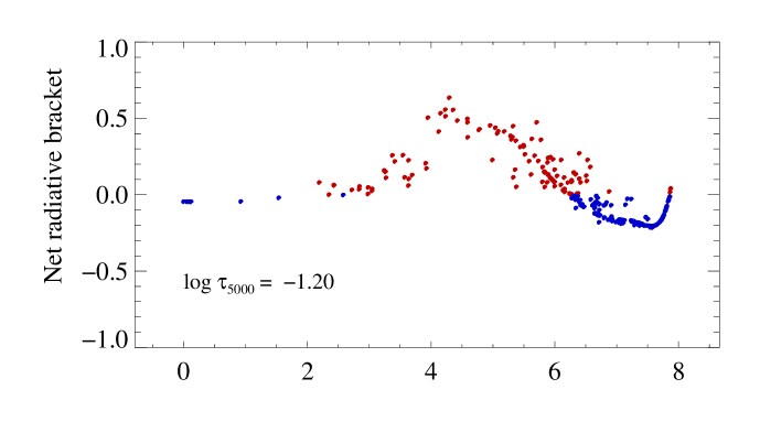
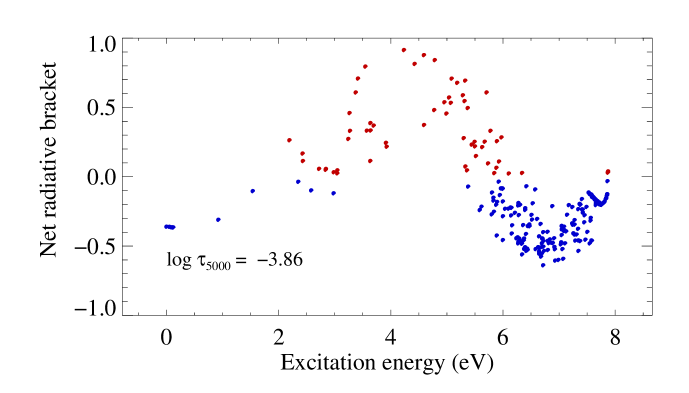
In the layers with $\log\tau_{\rm 5000}<-1$, the dominant mechanism is over-ionization from the Fe i levels with excitation energies at $2-5$ eV. The lower-lying levels, including the ground state of Fe i, maintain underpopulation due to radiative and collisional coupling with the former. Excitation balance of Fe i is also mildly affected by radiative imbalances in line transitions. These include radiative pumping by the non-local UV radiative field, as well as photon suction driven by photon losses in large-probability Fe i transitions between highly-excited levels. These processes leave a characteristic imprint on the behavior of $b_{i}$-factors in the outer atmospheric layers, $\log\tau_{\rm 5000}<-2$. In the infrared continuum, $J_{\nu}<B_{\nu}$ leads to over-recombination, which is very efficient for our atomic model with only $0.03$ eV energy gap of the upper Fe i levels from the Fe ii ground state. This is illustrated in Fig. 4, which shows net radiative brackets for all Fe i levels in the model atom at the depths $\log\tau_{\rm 5000}=0.12$, $-1.2$, and $-3.86$. All Fe i levels with excitation energy between $2$ and $6$ eV experience net over-ionization, and the loop is closed by net over-recombination to the upper levels. Note that only radiative rates are plotted. We also compared absolute radiative rates from multi and detail and found that they agree very well with each other.

Figure 5: Total number densities of Fe i/Fe ii for the Sun, HD 140283, HD 84937, and HD 122563.

Figure 6: Mean radiation field compared to the local Planck function in the UV continuum computed with the 1D and $\langle 3\rm{D}\rangle$ model atmospheres of the metal-poor sub-giant HD 140283.

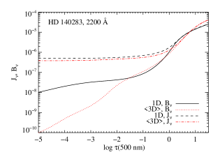
A comparison of the departure coefficients computed with 1D and $\langle 3\rm{D}\rangle$ model atmospheres reveals important differences (Fig. 3), which depend on stellar parameters, although their qualitative behavior is the same. Generally, metal-poor $\langle 3\rm{D}\rangle$ models show more thermalization close to continuum-forming layers, while in the outer layers Fe i atoms experience a larger degree of over-ionization. This can be primarily understood based on the temperature gradients, which in the $\langle 3\rm{D}\rangle$ stratifications are shallower in the inner layers but steeper in the outer layers compared to 1D models. We briefly consider the case of the metal-poor subgiant HD 140283, for which the 1D and $\langle 3\rm{D}\rangle$ model atmospheres are compared in Fig. 1. The $\langle 3\rm{D}\rangle$ model leads to smaller deviations from LTE at $-2\lesssim\log\tau_{\rm 5000}\lesssim 0$. That is, for the majority of the underpopulated Fe i levels, $b_{i}$(1D) $<$ $b_{i}$($\langle 3\rm{D}\rangle$). Inspection of the respective T$(\tau)$ relations in Fig. 1 shows that the $\langle 3\rm{D}\rangle$ model is cooler than the marcs model at $0\lesssim\log\tau_{\rm 5000}\lesssim 1$, where the UV continua form, but it is $\sim 100$ K hotter higher up. Figure 6 illustrates mean angle-averaged intensities at $2200$ Å, i.e., at the wavelength sampled by the ionization edges of the important Fe i levels. These are shown for the 1D and $\langle 3\rm{D}\rangle$ models, and are compared with the local Planck functions $B_{\nu}$ at each optical depth. At $-1.5\lesssim\log\tau_{\rm 5000}\lesssim 0$, the $J_{\nu}-B_{\nu}$ imbalance is smaller in the $\langle 3\rm{D}\rangle$ model compared to the 1D model, and, thus, over-ionization is less efficient. In this range of optical depths, densities in the $\langle 3\rm{D}\rangle$ stratification are also slightly larger than in the 1D model (Fig. 1). At $\log\tau_{\rm 5000}\lesssim-2$, the situation is reverse. The $\langle 3\rm{D}\rangle$ model is nearly $1000$ K cooler and less dense than the 1D model. The $J_{\nu}-B_{\nu}$ imbalance becomes very large causing significant underpopulation of the lower Fe i levels, while uppermost Fe i levels and the Fe ii ground state and excited levels develop appreciable overpopulation compared to their LTE occupation numbers. In contrast, 1D models predict nearly thermalized Fe ii level populations, over the whole optical depth scale.

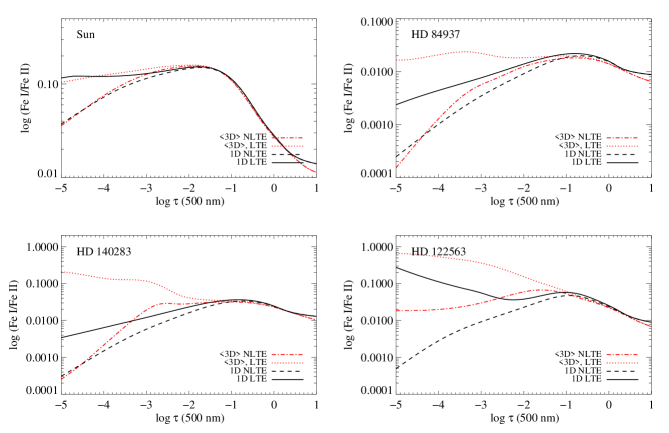
Figure 5 shows the ratios of Fe i/Fe ii number densities for the four cases: marcs and $\langle 3\rm{D}\rangle$ model atmospheres, NLTE and LTE. In the LTE case, about $\sim 5-10$ percent of the element is in the form of Fe i above $\log\tau_{\rm 5000}\sim 0$. In the $\langle 3\rm{D}\rangle$ models, due to their steeper T($\tau$) relation, LTE recombination of Fe ii to Fe i is even more efficient, raising Fe i/Fe ii to $20-50$ percent. Under NLTE, this effect is suppressed since ionization balance is primarily set by radiative ionization and recombination. For the metal-poor stars, Fe i occupies less then $1$ percent of the total element abundance at $\log\tau_{\rm 5000}<-2$ notwithstanding much cooler outer layers of the $\langle 3\rm{D}\rangle$ models. We note, however, that the huge differences in the ionization balance of Fe i/Fe ii in the outer layers of the models are not important for our NLTE abundance determinations. Most of the Fe i lines observed in spectra of the selected metal-poor stars form close to the continuum forming regions, $-2<\log\tau_{\rm 5000}<0$.

Extensive tests demonstrated that the behavior of departure coefficients is robust against the differences in terms of model atmospheres and NLTE codes used for the statistical equilibrium calculations. Perhaps, the only systematic effect is that multi predicts slightly stronger NLTE effects than detail mainly due to the differences in the background opacity. Also, the comparison of the LTE and NLTE equivalent widths obtained with multi and detail/siu show agreement to within $1-5$ percent for the lines with $W_{\lambda}>10~{}{\rm m\AA}$; NLTE $W_{\lambda}$’s are somewhat divergent for the weakest lines, with the relative $(\textsc{multi}-\textsc{detail})$ differences being about $10$ percent. These differences shall be taken as a formal error, which arises as a consequence of different implementations of the same basic physics in the various codes. Still, this is not of a big concern in our work because the calibration of the models and grid calculations are consistently performed with same code (multi). Furthermore, the magnitude of the NLTE effects is initially effectively controlled by a free parameter, the scaling factor $S\!_{\rm H}$ for the efficiency of the H i collisions.

4 Spectroscopic stellar parameters

4.1 Method

Spectroscopic stellar parameters, including metallicity, effective temperature, gravity, and microturbulence, were determined for each model atmosphere (marcs, mafags, $\langle 3\rm{D}\rangle$) in LTE and NLTE using the following approach.

In a first step, we performed full spectrum synthesis for the reference stars with the siu line formation code using the 1D mafags-os model atmospheres computed with parameters described in Sect. 4.2. The mafags-os models were used at this stage because they include partial pressures for molecules, which are important contributors to the background opacity of cooler stars. The profiles of all diagnostic Fe lines computed in LTE and NLTE were visually fitted to the observed spectra. The lines were computed with depth-dependent Voigt profiles taking into account various external broadening mechanisms. The equivalent widths of the Fe lines were then obtained from the best-fitting NLTE profiles, excluding contribution of blends. The $W_{\lambda}$’s are given in Tables 8 and 9 of the Appendix and are accurate to within $1-2$ percent.

In a second step, the equivalent widths $W_{\lambda}$’s were applied to determine spectroscopic parameters using the grids of LTE and NLTE equivalent widths computed with multi for marcs and $\langle 3\rm{D}\rangle$ model atmospheres. For each star, we constructed a local model atmosphere grid with two effective temperature points (the IRFM value and a value $200$ K lower), two values of microturbulence ($1$ and $2$ km s^-1), and a range of plausible metallicities ($\Delta$[Fe/H] up to $\pm 1.5$ dex) with a step-size of $0.25$ dex. Equivalent widths were computed for the grid models in LTE as well as in NLTE for two values of the H i collision efficiency parameter, $S\!_{\rm H}=0.1$ and $S\!_{\rm H}=1$. In order to save computational time in the construction of the local model grids in the $\langle 3\rm{D}\rangle$ case, the $\langle 3\rm{D}\rangle$ models were simply adjusted by multiplying the temperature and electron pressure at a given optical depth with the ratios of those quantities obtained from corresponding 1D models. Based on our experience with scaling 1D and 3D model stellar atmospheres to different stellar parameters, this procedure appears accurate to first-order level. The grid was thus constructed for marcs and $\langle 3\rm{D}\rangle$ models.

mafags-os model parameters were adjusted by assuming the equivalent widths to have the same sensitivity to stellar parameters as for marcs model, which is reasonable considering the similarity between the two codes.

An iterative procedure was then applied to determine spectroscopic parameters from Fe i and Fe i lines. First of all the microturbulent velocity was determined by flattening the slope of Fe ii line abundances with reduced equivalent width, thereby circumventing differential NLTE effects with line strength of Fe i lines. Only for the most metal-poor star G 64-12, the microturbulence is poorly defined due to the lack of strong Fe ii lines. We then followed two different approaches, keeping either $\log g$ or $T_{\mathrm{eff}}$ fixed, and optimizing the other parameter to establish ionization balance between the Fe i and Fe ii lines. In order to avoid biased results, we have not attempted to adjust the oscillator strengths of the Fe lines, giving preference to the experimental data from the laboratory measurements, or their weighted means if few measurements were available (Sect. 4.3). Hence, all abundance results are absolute values. Furthermore, we did not perform a differential stellar abundance analysis with respect to the Sun. First, that would conflict with the use of the reference stars as a calibration sample. Second, a differential approach would introduce yet an another source of error related to the usual problems of fitting the strong Fe lines in the solar spectrum, in particular the ambiguity between the effect of van der Waals damping and abundance on a line profile.

The standard technique to infer effective temperatures by flattening the slope of Fe i line abundances with excitation potential is particularly sensitive to the choice of transition probabilities. We found, however, that it is only weakly sensitive to $S\!_{\rm H}$, which is the main parameter we seek to constrain. Initial attempts to vary all parameters simultaneously, i.e. microturbulence from line strengths, effective temperature by excitation balance and surface gravity by ionization balance, did not give a conclusive answer in terms of the best choice of $S\!_{\rm H}$. This apparent weakness is likely related to the problem of multidimensionality in the parameter space, and, as such, shall be inherent to the method itself. In addition, we do not exclude remaining systematic uncertainties in the atomic and atmospheric models. It is possible that a differential approach between similar stars would be more successful in establishing temperatures based on excitation balance. We therefore reduced the dimensionality of the problem by not enforcing strict excitation equilibrium and focusing only on the ionization balance, as described above. As the results will show, an adequately flat trend with excitation potential is anyway naturally achieved for the majority of stars, HD 122563 being a notable exception.

The analysis described above was applied to each star in the sample using the marcs, mafags, and $\langle 3\rm{D}\rangle$ model atmospheres, thus yielding four desired quantities: $T_{\mathrm{eff}}$, $\log g$, [Fe/H], and $\xi_{\rm{t}}$. The results are discussed in Sect. 4.5. Table 5 gives the mean metallicities determined using the reference $T_{\mathrm{eff}}$ and $\log g$, and abundances averaged over the measured Fe i and Fe ii lines together with their standard deviations are presented in Table 7.

4.2 Observations and reference stellar parameters

Our reference sample consists of six late-type stars (Table 1), and includes two solar-metallicity stars (the Sun and Procyon), two metal-poor dwarfs (HD 84937 and G 64-12), a metal-poor subgiant (HD 140283), and a very bright metal-poor giant (HD 122563). The following observed spectra were adopted here. For the Sun, we used the KPNO flux spectrum (Kurucz et al. 1984). The UVES observations of Procyon (HD 61421), HD 84937, HD 140283, and HD 122563 were taken from the UVES-POP survey (Bagnulo et al., 2003). These spectra have a slit-determined resolution of $\lambda/\Delta\lambda\sim 80\,000$ and a signal-to-noise ratio $S/N\sim 300$ near $5000$ Å. The UVES spectrum for G 64-12 was taken from ESO/ST-ECF Science Archive Facility (67.D-0554(A)). The number of Fe lines suitable for the spectrum synthesis at this spectral quality, is $40$ (Procyon) to $10$ (G 64-12). For comparison, we also used the Keck/HIRES spectra of G 64-12 with $\lambda/\Delta\lambda\sim 100\,000$ and $S/N\sim 500$ kindly provided by J. Melendez (private communication).

A crucial step in our analysis is the choice of the reference $T_{\mathrm{eff}}$ and $\log g$ values for the selected stars, which are used as a benchmark for testing the new NLTE model atom and $\langle 3\rm{D}\rangle$ model atmospheres. These parameters were taken from the literature, giving preference to the least model-dependent methods, such as interferometry, infra-red flux method (IRFM), and parallaxes. The adopted values and their uncertainties are given in the Table 1. A brief description of these data is given below.

Table 1: Input parameters for the reference stars. Parallaxes $\pi$ and their uncertainties are also given. See text.

Star	$T_{\rm eff}$	$\sigma$	Ref.	$\log g$	$\sigma$	$\pi$	$\sigma$	[Fe/H]
Sun	$5777$			$4.44$
Procyon	$6543$	84	a	$3.98$	0.02	284.56	1.26	-0.03
HD 84937	$6408$	66	b	$4.13$	0.09	3.83	0.78	-2.16
HD 140283	$5777$	55	b	$3.70$	0.08	17.16	0.68	-2.38
HD 122563	$4665$	80	c	$1.64$	0.16	4.22	0.35	-2.51
G 64-12	$6464$	61	b	$4.3^{*}$		0.57	2.83	-3.12

References: a - Aufdenberg et al. (2005); b - Casagrande et al. (2010); c - Casagrande (private communication)
^∗ $\log g$ is derived from the upper limit on the parallax

For the four metal-poor stars, we adopted the IRFM effective temperatures by Casagrande et al. (2010). The mean internal uncertainty of the data is about $70$ K, which includes the uncertainty on the zero point of the $T_{\mathrm{eff}}$ scale, reddening and photometric errors.

The IRFM value for the metal-poor giant HD 122563, $T_{\mathrm{eff}}=4665\pm 80$ K, was kindly provided by L. Casagrande (private communication). This estimate incorporates a correction due to reddening, $E(B-V)=0.005$, which was determined from the interstellar Na D lines detected in the UVES spectrum. Our equivalent widths for the $5889.95$ and $5895.92$ Å Na i lines are $22.3$ and $12.4$ mÅ, respectively.

For Procyon, an interferometric estimate of angular diameter is available (Aufdenberg, Ludwig & Kervella, 2005), which gives $T_{\mathrm{eff}}=6545\pm 83$ K and combined with a very accurate parallax $\pi=284.56\pm 1.26$ milli-arcsec, surface gravity can be estimated, $\log g=3.99\pm 0.02$.

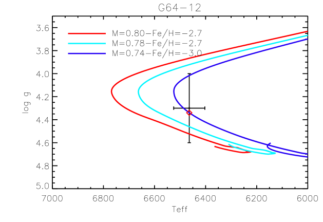
For the other stars, we determined surface gravities from the Hipparcos parallaxes (van Leeuwen, 2007) using the masses estimated from the tracks of VandenBerg et al. (2000) by Gehren et al. (2004, 2006) and apparent bolometric magnitudes from Casagrande et al. (2010). The uncertainties were computed by mapping the uncertainty in mass (0.2 M_⊙ for HD 122563 and G 64-12, and $0.1$ M_⊙ for HD 84937 and HD 140283), temperature and parallax into the range of possible gravities ($\Delta\log g\leq 0.16$ dex). The only exception is G 64-12, for which the parallax is too uncertain, $\pi=0.57\pm 2.83$ milli-arcsec. From comparison with metal-poor evolutionary tracks for reasonable masses (Fig. 11), one may also conclude that within the errors of the given $T_{\mathrm{eff}}$ ($6464$ K) surface gravity of G 64-12 is in the range $\log g=3.8\ldots 4.6$ dex. We, thus adopt the value derived from the upper limit on the parallax, $\log g=4.3$ and assign a nominal error of $0.3$ dex. In comparison, Nissen, Chen, Asplund & Pettini (2004, 2007) and Fabbian, Nissen, Asplund, Pettini & Akerman (2009) estimate $\log g=4.26$.

4.3 Line selection

Table 2: Parameters of the Fe i lines used for the solar analysis.

$\lambda$	Lower	Upper	gl	gu	$E_{\rm low}$	$\log gf$	$\log C_{6}$
$\AA$	level	level			[eV]
4445.47	$a\,^{5}{\rm D}$	$z\,^{7}{\rm F}^{{\rm\circ}}$	5	5	0.09	-5.410	-31.8
4494.56	$a\,^{5}{\rm P}$	$x\,^{5}{\rm D}^{{\rm\circ}}$	5	7	2.20	-1.136	-31.2
4920.50	$z\,^{7}{\rm F}^{{\rm\circ}}$	$e\,^{7}{\rm D}$	11	9	2.80	0.068	-30.5
4994.13	$a\,^{5}{\rm F}$	$z\,^{5}{\rm F}^{{\rm\circ}}$	9	7	0.92	-3.080	-31.7
5044.21	$z\,^{7}{\rm F}^{{\rm\circ}}$	$e\,^{7}{\rm D}$	9	11	2.85	-2.017	-30.6
5198.71	$a\,^{5}{\rm P}$	$y\,^{5}{\rm P}^{{\rm\circ}}$	3	5	2.22	-2.135	-31.3
5216.27	$a\,^{3}{\rm F}$	$z\,^{3}{\rm F}^{{\rm\circ}}$	5	5	1.61	-2.150	-31.5
5225.53	$a\,^{5}{\rm D}$	$z\,^{7}{\rm D}^{{\rm\circ}}$	3	3	0.11	-4.789	-31.9
5232.94	$z\,^{7}{\rm P}^{{\rm\circ}}$	$e\,^{7}{\rm D}$	9	11	2.94	-0.060	-30.6
5236.20	$c\,^{3}{\rm F}$	$t\,^{3}{\rm D}^{{\rm\circ}}$	5	3	4.19	-1.497	-31.3
5242.49	$a\,^{1}{\rm I}$	$z\,^{1}{\rm H}^{{\rm\circ}}$	13	11	3.63	-0.967	-31.3
5247.05	$a\,^{5}{\rm D}$	$z\,^{7}{\rm D}^{{\rm\circ}}$	5	7	0.09	-4.960	-31.9
5250.21	$a\,^{5}{\rm D}$	$z\,^{7}{\rm D}^{{\rm\circ}}$	1	3	0.12	-4.938	-31.9
5269.54	$a\,^{5}{\rm F}$	$z\,^{5}{\rm D}^{{\rm\circ}}$	11	9	0.86	-1.321	-31.8
5281.79	$z\,^{7}{\rm P}^{{\rm\circ}}$	$e\,^{7}{\rm D}$	5	7	3.04	-0.830	-30.5
5379.57	$b\,^{1}{\rm G}$	$z\,^{1}{\rm H}^{{\rm\circ}}$	9	11	3.70	-1.514	-31.3
5383.37	$z\,^{5}{\rm G}^{{\rm\circ}}$	$e\,^{5}{\rm H}$	11	13	4.31	0.645	-30.4
5434.52	$a\,^{5}{\rm F}$	$z\,^{5}{\rm D}^{{\rm\circ}}$	3	1	1.01	-2.122	-31.7
5491.84	$c\,^{3}{\rm F}$	$u\,^{3}{\rm D}^{{\rm\circ}}$	5	7	4.19	-2.190	-30.4
5600.22	$z\,^{3}{\rm P}^{{\rm\circ}}$	$g\,^{5}{\rm D}$	3	3	4.26	-1.420	-30.4
5661.35	$z\,^{3}{\rm P}^{{\rm\circ}}$	$g\,^{5}{\rm D}$	1	3	4.28	-1.756	-31.3
5662.52	$y\,^{5}{\rm F}^{{\rm\circ}}$	$g\,^{5}{\rm D}$	11	9	4.18	-0.573	-30.5
5696.09	$y\,^{3}{\rm F}^{{\rm\circ}}$	$e\,^{5}{\rm H}$	9	9	4.55	-1.720	-30.2
5701.54	$b\,^{3}{\rm F}$	$y\,^{3}{\rm D}^{{\rm\circ}}$	9	7	2.56	-2.163	-31.3
5705.46	$y\,^{5}{\rm F}^{{\rm\circ}}$	$g\,^{5}{\rm D}$	3	3	4.30	-1.360	-30.5
5778.45	$b\,^{3}{\rm F}$	$y\,^{3}{\rm D}^{{\rm\circ}}$	7	7	2.59	-3.440	-31.3
5855.08	$y\,^{3}{\rm F}^{{\rm\circ}}$	$e\,^{5}{\rm H}$	7	9	4.61	-1.480	-30.3
5916.25	$a\,^{3}{\rm H}$	$y\,^{3}{\rm F}^{{\rm\circ}}$	9	9	2.45	-2.994	-31.4
5956.69	$a\,^{5}{\rm F}$	$z\,^{7}{\rm P}^{{\rm\circ}}$	11	9	0.86	-4.550	-31.8
6065.48	$b\,^{3}{\rm F}$	$y\,^{3}{\rm F}^{{\rm\circ}}$	5	5	2.61	-1.530	-31.3
6082.71	$a\,^{5}{\rm P}$	$z\,^{3}{\rm P}^{{\rm\circ}}$	3	3	2.22	-3.570	-31.5
6151.62	$a\,^{5}{\rm P}$	$y\,^{5}{\rm D}^{{\rm\circ}}$	7	5	2.18	-3.282	-31.6
6173.33	$a\,^{5}{\rm P}$	$y\,^{5}{\rm D}^{{\rm\circ}}$	3	1	2.22	-2.880	-31.6
6200.31	$b\,^{3}{\rm F}$	$y\,^{3}{\rm F}^{{\rm\circ}}$	5	7	2.61	-2.416	-31.3
6219.28	$a\,^{5}{\rm P}$	$y\,^{5}{\rm D}^{{\rm\circ}}$	5	5	2.20	-2.433	-31.6
6240.65	$a\,^{5}{\rm P}$	$z\,^{3}{\rm P}^{{\rm\circ}}$	3	5	2.22	-3.287	-31.5
6252.56	$a\,^{3}{\rm H}$	$z\,^{3}{\rm G}^{{\rm\circ}}$	13	11	2.40	-1.687	-31.4
6265.13	$a\,^{5}{\rm P}$	$y\,^{5}{\rm D}^{{\rm\circ}}$	7	7	2.18	-2.547	-31.6
6297.79	$a\,^{5}{\rm P}$	$y\,^{5}{\rm D}^{{\rm\circ}}$	3	5	2.22	-2.715	-31.6
6311.50	$b\,^{3}{\rm P}$	$y\,^{3}{\rm D}^{{\rm\circ}}$	5	5	2.83	-3.141	-31.4
6430.85	$a\,^{5}{\rm P}$	$y\,^{5}{\rm D}^{{\rm\circ}}$	7	9	2.18	-2.006	-31.6
6498.94	$a\,^{5}{\rm F}$	$z\,^{7}{\rm F}^{{\rm\circ}}$	7	7	0.96	-4.695	-31.8
6518.37	$b\,^{3}{\rm P}$	$y\,^{3}{\rm D}^{{\rm\circ}}$	5	7	2.83	-2.298	-31.4
6574.23	$a\,^{5}{\rm F}$	$z\,^{7}{\rm F}^{{\rm\circ}}$	5	5	0.99	-5.010	-32.4
6593.87	$a\,^{3}{\rm H}$	$z\,^{5}{\rm G}^{{\rm\circ}}$	11	11	2.43	-2.394	-31.4
6609.11	$b\,^{3}{\rm F}$	$z\,^{3}{\rm G}^{{\rm\circ}}$	9	9	2.56	-2.682	-31.4
6699.14	$d\,^{3}{\rm F}$	$u\,^{3}{\rm D}^{{\rm\circ}}$	9	7	4.59	-2.101	-31.5
6726.67	$y\,^{5}{\rm P}^{{\rm\circ}}$	$e\,^{5}{\rm P}$	5	3	4.61	-1.000	-30.5
6739.52	$a\,^{3}{\rm F}$	$z\,^{5}{\rm F}^{{\rm\circ}}$	7	7	1.56	-4.794	-31.7
6750.15	$a\,^{3}{\rm P}$	$z\,^{3}{\rm P}^{{\rm\circ}}$	3	3	2.42	-2.605	-31.4
6793.26	$c\,^{3}{\rm F}$	$w\,^{5}{\rm G}^{{\rm\circ}}$	9	9	4.08	-2.326	-30.8
6810.26	$y\,^{5}{\rm P}^{{\rm\circ}}$	$e\,^{5}{\rm P}$	5	7	4.61	-0.986	-30.4
6837.01	$d\,^{3}{\rm F}$	$u\,^{3}{\rm G}^{{\rm\circ}}$	9	9	4.59	-1.690	-31.6
6854.82	$d\,^{3}{\rm F}$	$3\,^{H}{\rm P}$	9	11	4.59	-1.926	-31.6
6945.20	$a\,^{3}{\rm P}$	$z\,^{3}{\rm P}^{{\rm\circ}}$	3	5	2.42	-2.454	-31.4
6978.85	$a\,^{3}{\rm P}$	$z\,^{3}{\rm P}^{{\rm\circ}}$	1	3	2.48	-2.480	-31.4
7401.68	$c\,^{3}{\rm F}$	$w\,^{3}{\rm D}^{{\rm\circ}}$	5	3	4.19	-1.500	-31.2
7912.87	$a\,^{5}{\rm F}$	$z\,^{7}{\rm D}^{{\rm\circ}}$	11	9	0.86	-4.848	-31.9
8293.51	$a\,^{3}{\rm D}$	$y\,^{3}{\rm D}^{{\rm\circ}}$	5	5	3.30	-2.203	-31.3

Table 3: Parameters of the Fe ii lines used for the solar analysis.

$\lambda$	Lower	Upper	gl	gu	$E_{\rm low}$	$\log gf$	$\log C_{6}$
$\AA$	level	level			[eV]
4491.40	$b\,^{4}{\rm F}$	$z\,^{4}{\rm F}^{{\rm\circ}}$	4	4	2.856	-2.71	-32.1
4508.29	$b\,^{4}{\rm F}$	$z\,^{4}{\rm D}^{{\rm\circ}}$	4	2	2.856	-2.44	-32.0
4576.34	$b\,^{4}{\rm F}$	$z\,^{4}{\rm D}^{{\rm\circ}}$	6	6	2.844	-2.95	-32.0
4582.84	$b\,^{4}{\rm F}$	$z\,^{4}{\rm F}^{{\rm\circ}}$	6	8	2.844	-3.18	-32.1
4583.84	$b\,^{4}{\rm F}$	$z\,^{4}{\rm F}^{{\rm\circ}}$	10	8	2.807	-1.93	-32.0
4620.52	$b\,^{4}{\rm F}$	$z\,^{4}{\rm D}^{{\rm\circ}}$	8	8	2.828	-3.21	-32.0
4923.93	$a\,^{6}{\rm S}$	$z\,^{6}{\rm P}^{{\rm\circ}}$	6	4	2.891	-1.26	-32.1
5018.44	$a\,^{6}{\rm S}$	$z\,^{6}{\rm P}^{{\rm\circ}}$	6	6	2.891	-1.10	-32.1
5169.03	$a\,^{6}{\rm S}$	$z\,^{6}{\rm P}^{{\rm\circ}}$	6	8	2.891	-1.00	-32.1
5197.58	$a\,^{4}{\rm G}$	$z\,^{4}{\rm F}^{{\rm\circ}}$	6	4	3.230	-2.22	-32.1
5234.62	$a\,^{4}{\rm G}$	$z\,^{4}{\rm F}^{{\rm\circ}}$	8	6	3.221	-2.18	-32.1
5264.81	$a\,^{4}{\rm G}$	$z\,^{4}{\rm D}^{{\rm\circ}}$	6	4	3.230	-3.13	-32.0
5284.11	$a\,^{6}{\rm S}$	$z\,^{6}{\rm F}^{{\rm\circ}}$	6	8	2.891	-3.11	-32.1
5325.55	$a\,^{4}{\rm G}$	$z\,^{4}{\rm F}^{{\rm\circ}}$	8	8	3.221	-3.16	-32.1
5414.07	$a\,^{4}{\rm G}$	$z\,^{4}{\rm D}^{{\rm\circ}}$	8	8	3.221	-3.58	-32.0
5425.26	$a\,^{4}{\rm G}$	$z\,^{4}{\rm F}^{{\rm\circ}}$	10	10	3.199	-3.22	-32.1
6239.95	$b\,^{4}{\rm D}$	$z\,^{4}{\rm P}^{{\rm\circ}}$	2	4	3.889	-3.41	-32.0
6247.56	$b\,^{4}{\rm D}$	$z\,^{4}{\rm P}^{{\rm\circ}}$	6	4	3.892	-2.30	-32.0
6369.46	$a\,^{6}{\rm S}$	$z\,^{6}{\rm D}^{{\rm\circ}}$	6	4	2.891	-4.11	-32.1
6432.68	$a\,^{6}{\rm S}$	$z\,^{6}{\rm D}^{{\rm\circ}}$	6	6	2.891	-3.57	-32.1
6456.38	$b\,^{4}{\rm D}$	$z\,^{4}{\rm P}^{{\rm\circ}}$	8	6	3.903	-2.05	-32.0
6516.08	$a\,^{6}{\rm S}$	$z\,^{6}{\rm D}^{{\rm\circ}}$	6	8	2.891	-3.31	-32.1
7222.39	$b\,^{4}{\rm D}$	$z\,^{4}{\rm D}^{{\rm\circ}}$	4	2	3.889	-3.26	-32.0
7224.49	$b\,^{4}{\rm D}$	$z\,^{4}{\rm D}^{{\rm\circ}}$	2	2	3.889	-3.20	-32.0
7515.83	$b\,^{4}{\rm D}$	$z\,^{4}{\rm D}^{{\rm\circ}}$	8	6	3.903	-3.39	-32.0
7711.72	$b\,^{4}{\rm D}$	$z\,^{4}{\rm D}^{{\rm\circ}}$	8	8	3.903	-2.50	-32.0

Table 4: Parameters of the Fe I lines used for the abundance analysis of the metal-poor stars. $gf$-values are taken from NIST.

$\lambda$	Lower	Upper	gl	gu	$E_{\rm low}$	$\log gf$	$\log C_{6}$
$\AA$	level	level			[eV]
3581.19	$a\,^{5}{\rm F}$	$z\,^{5}{\rm G}^{{\rm\circ}}$	11	13	0.86	0.406	-31.6
3618.77	$a\,^{5}{\rm F}$	$z\,^{5}{\rm G}^{{\rm\circ}}$	5	7	0.99	-0.003	-31.5
3719.93	$a\,^{5}{\rm D}$	$z\,^{5}{\rm F}^{{\rm\circ}}$	9	11	0.00	-0.432	-31.8
3737.13	$a\,^{5}{\rm D}$	$z\,^{5}{\rm F}^{{\rm\circ}}$	7	9	0.05	-0.574	-31.6
3745.56	$a\,^{5}{\rm D}$	$z\,^{5}{\rm F}^{{\rm\circ}}$	5	7	0.09	-0.771	-31.8
3758.23	$a\,^{5}{\rm F}$	$y\,^{5}{\rm F}^{{\rm\circ}}$	7	7	0.96	-0.027	-31.6
3820.43	$a\,^{5}{\rm F}$	$y\,^{5}{\rm D}^{{\rm\circ}}$	11	9	0.86	0.119	-31.6
4045.81	$a\,^{3}{\rm F}$	$y\,^{3}{\rm F}^{{\rm\circ}}$	9	9	1.49	0.280	-31.5
4235.94	$z\,^{7}{\rm D}^{{\rm\circ}}$	$e\,^{7}{\rm D}$	9	9	2.43	-0.341	-30.5
4250.79	$a\,^{3}{\rm F}$	$z\,^{3}{\rm G}^{{\rm\circ}}$	7	7	1.56	-0.714	-31.5
4415.12	$a\,^{3}{\rm F}$	$z\,^{5}{\rm G}^{{\rm\circ}}$	5	7	1.61	-0.615	-31.5
5586.76	$z\,^{5}{\rm F}^{{\rm\circ}}$	$e\,^{5}{\rm D}$	9	7	3.37	-0.144	-30.4

The Fe lines for the abundance calculations were selected on a star by star basis, i.e., carefully inspecting the observed stellar spectra. We rejected lines affected by blends, strong damping wings or are located in the spectral windows where continuum placement is uncertain. Our solar line list includes $59$ lines of Fe i and $24$ lines of Fe ii in the wavelength range $4400-8500$ Å. In spectra of the metal-poor stars most of these lines are very weak. Thus, $12$ strong lines of Fe i were added to the analysis of the metal-poor stars. All line parameters are given in Tables 2, 3, and 4.

The $gf$-values adopted in this work are weighted averages of different experimental values. An elaborate discussion of their accuracy can be found in Gehren et al. (2001). The largest weights are typically assigned to the $\log gf$ values measured at Oxford (Blackwell et al. 1979; Blackwell, Petford & Shallis 1979; Blackwell & Shallis 1979; Blackwell et al. 1980; Blackwell, Shallis & Simmons 1982; Blackwell et al. 1982; Blackwell, Petford & Simmons 1982; Blackwell et al. 1986). According to the NIST database, the uncertainties of the data are $3-10\%$. Smaller weights are assigned to the $gf$-values of the Hannover group (Bard, Kock & Kock 1991, Bard & Kock 1994, uncertainties typically $10-25\%$) and O’Brian et al. (1991, uncertainties $25-50\%$). The $gf$-values for the Fe ii transitions are taken from Meléndez & Barbuy (2009), who renormalized the branching fractions from Raassen & Uylings (1998) and other theoretical sources to the experimental lifetimes (Schnabel et al. 1999, e.g., that of ; Schnabel et al. 2004, e.g., that of ). To avoid biased results, we excluded any of their ’solar’ values, which were obtained by a 1D LTE spectroscopic analysis of the solar flux spectrum. That is, for the Fe ii transitions $\lambda\lambda\ 5284.1,6239.95,6247.56,6456.38\ \AA$ we kept the NIST-recommended values.

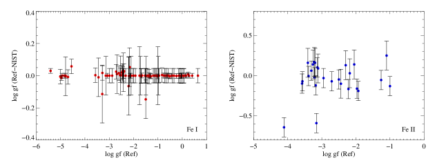
Our adopted transition probabilites for the Fe i and Fe ii lines are compared to the NIST-recommended values in Fig. 7. There are small differences for the weak Fe ii transitions, which reflect the discrepancies between the NIST Fe ii data based essentially on the Raassen & Uylings (1998) study and the adopted values of Meléndez & Barbuy (2009). Note that Grevesse & Sauval (1999) in the re-analysis of the solar Fe abundance discuss the possibility of underestimated $\log gf$’s from Raassen & Uylings (1998) for the optical lines, although they do not find the same problem for the Fe ii UV lines.

Figure 7: Comparison of transition probabilities adopted in this work (Ref) with that from the NIST database.

Line broadening due to elastic collisions with H i atoms was computed from the tables of Barklem, Piskunov & O’Mara (2000) and Barklem & Aspelund-Johansson (2005). For the four Fe i lines ($4445.47$, $5600.22$, $5661.35$, $8293.51$ Å), broadening cross-sections $\sigma$ and their velocity dependence $\alpha$ were kindly provided by P. Barklem (2011, private communication). For seven lines, the Unsold (1955) values increased by a factor of $1.5$ were adopted. In Tables 2, 3, and and 4 these values are given in terms of commonly-used van der Waals damping constants $\log C_{6}$.

4.4 Sun and Procyon

Owing to the superior quality of the solar spectrum, the initial spectrum synthesis for the Sun was performed taking into account solar rotation with $V_{\rm rot,\odot}=1.8$ km s^-1  and a radial-tangential macroturbulence velocity $\xi_{\rm{RT}}$, which was adjusted for each line separately. The typical values of $\xi_{\rm{RT}}$ required to match the observed spectrum are $2.5\ldots 4$ km s^-1 for the profile fitting with the 1D models, and $1.6\ldots 3$ km s^-1 for that with the $\langle 3\rm{D}\rangle$ model. We note that in full 3D line formation calculations Asplund et al. (2000) found that no macroturbulence was necessary to fit the line profiles due to the Doppler shifts from the convective motions, which are not explicitly taken into account in the $\langle 3\rm{D}\rangle$ models used here.

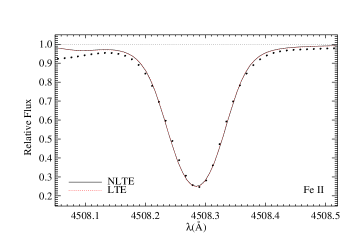
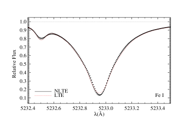
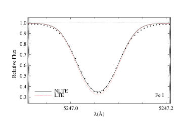
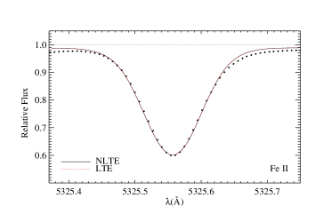
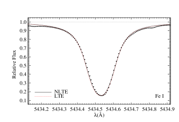
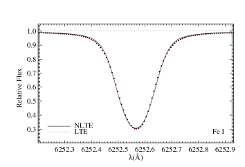
Selected Fe i and Fe ii solar line profiles computed under LTE and NLTE with the $\langle 3\rm{D}\rangle$ models are compared with the observations in Fig. 8. In general, NLTE Fe i line profiles are weaker compared to LTE, which is driven by the NLTE effect on the line opacity. For the strongest Fe i lines, forming very far out in the atmospheres, deviation of the line source function from the Planck function, $S_{\rm ij}<B_{\nu}(T_{\rm e})$, leads to line core darkening. However, their wings, which dominate the total line strength, are formed at the depths where $b_{i}<1$ due to over-ionization, and the NLTE absorption coefficient is smaller. Therefore the NLTE equivalent widths are smaller compared to LTE for a given abundance. As discussed in Sect. 3, NLTE effects on the Fe ii lines are negligible. We also inspected the influence of inelastic H i collisions on the line profiles finding that the profile shapes are rather insensitive to the $S\!_{\rm H}$ value. Any Fe line could be fitted by slightly adjusting the abundance or the damping parameters within the error bars (typically $10$ percent).

Figure 8: Synthetic (black trace) and observed (dots) profiles of selected Fe i and Fe ii lines in the solar flux spectrum. The results are shown for the mafags-os solar model in NLTE (black trace) and LTE (dotted trace).

The mean Fe abundances computed with the mafags-os, marcs, and the $\langle 3\rm{D}\rangle$ model atmospheres are given in the Table 5 (see also Fig. 12). The total errors of the mean are only shown for the NLTE results obtained with the $\langle 3\rm{D}\rangle$ models. The total error was computed as:

$$\sigma_{\rm tot}=\left((\sigma_{\rm tot,FeI}^{2}+\sigma_{\rm tot,FeII}^{2})/2\right)^{1/2}$$

where,

$$\sigma_{\rm tot,~{}Fe}=(\sigma_{\rm Fe}^{2}+\sigma_{\log gf,\rm{Fe}}^{2}+\sigma_{\rm\log g,Fe}^{2}+\sigma_{T_{\mathrm{eff}},\rm{Fe}}^{2})^{1/2}$$

The total error includes the following uncertainties: observational errors given by the standard deviation, errors stemming from the reference values of the surface gravity and effective temperatures (Table 1), and in the $\log gf$ values. For the latter, we adopted the uncertainties given by NIST and assumed they are uncorrelated, since the $gf$-values come from different sources in the literature. That is, the total uncertainty $\sigma_{\log gf}$ is decreased by a factor $\sqrt{N}$, where $N$ is the number of lines, and it takes into account the relative number of the Fe i and Fe ii lines analyzed per star.

We find that the excitation and ionization equilibrium of Fe in the Sun and Procyon is well satisfied under NLTE with both 1D and $\langle 3\rm{D}\rangle$ models (Fig. 12, Table 7). The statistical uncertainty of the mean abundance, which corresponds to the standard error of the line sample, is not larger than $0.01$ dex. Some lines with $W_{\lambda}>100\ {\rm m\AA}$ seem to indicate slightly lower abundances, by $\sim 0.03$ dex, compared to the rest of the sample both in 1D and $\langle 3\rm{D}\rangle$ modelling. We do not assign much weight to these lines. First, it is almost impossible to discern the influence of abundance, damping, and weak blends in the line wings. Second, their asymmetric profiles are clearly shaped by convective velocity fields, which are not accounted for in our models. As a consequence, it is hardly possible to assign a unique ’best-fitting’ abundance to such lines at all, that, in addition to a systematic error caused by the neglect of 3D effects, introduces subjectivity in abundance estimates.

The mean NLTE abundances of Fe in the Sun and Procyon, determined using the $\langle 3\rm{D}\rangle$ model atmospheres, are $7.46\pm 0.02$ respectively $7.43\pm 0.07$ dex. 1D models (marcs or mafags-os) yield slightly lower values, which are, however, all consistent within the total error. For the Sun, the latter only reflects the statistical uncertainty of the $gf$-values, as described above. We also find that adopting LTE or scaling down the cross-sections for inelastic collisions with H i by an order of magnitude, $S\!_{\rm H}=0.1$ does not yield any significant effect on the mean abundance. The difference between the two extreme cases $\Delta$(NLTE-LTE) is $\approx 0.02$ dex. Thus, based on the analysis of the solar-metallicity stars only it is not possible to single out the optimum value of $S\!_{\rm H}$. It turns out, however, that this problem can be solved using the metal-poor stars with reliable stellar parameters (Sect. 4.5).

Comparing our results with the published values of the Fe abundance in the Sun and Procyon, we find full agreement with all data obtained with similar techniques and model atmospheres. We list only few most recent examples. Meléndez & Barbuy (2009) using a $\langle 3\rm{D}\rangle$ solar model very similar to that adopted in this work and LTE approach obtain $\log\varepsilon_{\rm FeII,\odot}=7.45$ dex. The NLTE 1D estimate by Gehren et al. (2001) obtained using the mafags-odf (note the difference with the mafags-os version used here) models is $\log\varepsilon_{\rm Fe,\odot}=7.48...7.51$ dex. In the follow-up NLTE study with the mafags-os models, Mashonkina et al. (2011) find $\log\varepsilon_{\rm Fe,\odot}=7.41\ldots 7.56$ depending on the source of $gf$-values used for the Fe ii lines. For Procyon, Mashonkina et al. (2011) claim discrepant abundances from the NLTE analysis of the Fe i and Fe ii lines, $\log\varepsilon_{\rm FeI}=7.46\pm 0.07$ respectively $\log\varepsilon_{\rm FeII}=7.52\pm 0.05$ dex (their Table 3, solution $S\!_{\rm H}=0.1$) suggesting that either increasing $T_{\mathrm{eff}}$ by $80$ K or decreasing $\log g$ by $0.15$ dex may solve the problem. Their results for Procyon with $S\!_{\rm H}=1$, which is consistent with our study, are discrepant, $\log\varepsilon_{\rm FeI}=7.41\pm 0.07$ respectively $\log\varepsilon_{\rm FeII}=7.53\pm 0.05$ dex, which is most likely due to the different sources of $\log gf$ values for the Fe ii lines.

We emphasize that further, more detailed, comparison to these and other studies is not meaningful because of various methodical differences, such as atomic data, line selection, and microturbulence, to name just a few.

4.5 Analysis of metal-poor stars

Table 5: Metallicities [Fe/H] and microturbulence $\xi_{\rm{t}}$ (km s^-1) determined relative to the Sun for the reference stars. The $\xi_{\rm{t}}$ for the mafags models are identical to that obtained with the marcs models and are not shown. NLTE results refer to $S\!_{\rm H}=1$. The references to the $T_{\mathrm{eff}}$ and $\log g$ values are given in the Table 1. See text.

Star	fixed		derived $\rightarrow$
	$T_{\rm eff}$	$\log g$	marcs				mafags		$\langle 3\rm{D}\rangle$				$\sigma_{\rm tot}$
			NLTE	$\xi$	LTE	$\xi$	NLTE	LTE	NLTE	$\xi$	LTE	$\xi$	NLTE, $\langle 3\rm{D}\rangle$
Sun	$5777$	$4.44$	7.44	1.02	7.43	1.02	7.46	7.45	7.46	1.08	7.45	1.09	0.02
Procyon	$6543$	$3.98$	-0.06	1.93	-0.08	1.94	-0.05	-0.07	-0.03	2.05	-0.04	2.06	0.07
HD 84937	$6408$	$4.13$	-2.07	1.42	-2.10	1.43	-2.05	-2.09	-2.03	1.38	-2.12	1.35	0.08
HD 140283	$5777$	$3.70$	-2.38	1.26	-2.42	1.27	-2.40	-2.43	-2.40	1.18	-2.53	1.17	0.07
HD 122563	$4665$	$1.64$	-2.55	1.60	-2.60	1.61	-2.48	-2.52	-2.57	1.66	-2.66	1.67	0.24
G 64-12	$6464$	$4.30$	-3.12	1.75	-3.24	1.75	-3.16	-3.23	-3.10	1.75	-3.37	1.75	0.17

Table 6: Spectroscopic $T_{\mathrm{eff}}$, $\log g$, $\xi_{\rm{t}}$ (km s^-1), and [Fe/H] values. The parameters, which were kept fixed in the calculations, are given in the column 2.

Star	fixed	derived $\rightarrow$
	$\log g$/$T_{\rm eff}$	1D, LTE			1D, $S\!_{\rm H}=1$			1D, $S\!_{\rm H}=0.1$			$\langle 3\rm{D}\rangle$, LTE			$\langle 3\rm{D}\rangle$, $S\!_{\rm H}=1$			$\langle 3\rm{D}\rangle$, $S\!_{\rm H}=0.1$
Sun	4.44	5794	1.0	7.44	5780	1.0	7.45	5753	1.0	7.46	5805	1.1	7.47	5793 $\pm$ 35	1.1	7.47 $\pm$ 0.03	5775	1.0	7.48
Procyon	3.98	6631	1.9	-0.04	6578	1.9	-0.05	6487	1.9	-0.05	6576	2.0	-0.04	6546 $\pm$ 43	2.0	-0.04 $\pm$ 0.04	6499	2.0	-0.05
HD84937	4.13	6405	1.4	-2.11	6328	1.4	-2.13	6115	1.4	-2.16	6483	1.3	-2.08	6314 $\pm$ 69	1.4	-2.10 $\pm$ 0.07	6134	1.5	-2.12
HD140283	3.70	5772	1.2	-2.43	5703	1.2	-2.45	5510	1.2	-2.49	6078	1.2	-2.36	5820 $\pm$ 65	1.2	-2.38 $\pm$ 0.07	5586	1.3	-2.41
HD122563	1.64	4754	1.6	-2.51	4705	1.6	-2.51	4609	1.5	-2.49	4838	1.7	-2.53	4755 $\pm$ 59	1.7	-2.50 $\pm$ 0.14	4669	1.7	-2.48
G64-12	4.30	6592	1.8	-3.15	6471	1.8	-3.17	6006	1.8	-3.34	6757	1.8	-3.18	6439 $\pm$ 152	1.8	-3.17 $\pm$ 0.17	6258	1.8	-3.16
Sun	5777	4.40	1.0	7.44	4.43	1.0	7.45	4.48	1.0	7.47	4.38	1.0	7.46	4.40 $\pm$ 0.06	1.0	7.47 $\pm$ 0.03	4.44	1.0	7.48
Procyon	6543	3.81	1.9	-0.11	3.93	1.9	-0.07	4.08	1.9	-0.04	3.92	2.0	-0.05	3.99 $\pm$ 0.14	2.0	-0.04 $\pm$ 0.08	4.06	2.0	-0.02
HD84937	6408	4.14	1.4	-2.11	4.26	1.4	-2.07	4.57	1.4	-1.98	4.00	1.3	-2.12	4.28 $\pm$ 0.16	1.4	-2.04 $\pm$ 0.08	4.53	1.5	-1.95
HD140283	5777	3.72	1.2	-2.42	3.84	1.2	-2.39	4.21	1.2	-2.26	3.11	1.1	-2.59	3.63 $\pm$ 0.14	1.1	-2.41 $\pm$ 0.08	4.05	1.3	-2.26
HD122563	4665	1.22	1.6	-2.65	1.48	1.6	-2.57	1.83	1.6	-2.45	0.91	1.7	-2.74	1.31 $\pm$ 0.26	1.7	-2.59 $\pm$ 0.19	1.61	1.7	-2.48
G64-12	6464	4.06	1.8	-3.26	4.29	1.8	-3.18	4.90	1.8	-3.05	3.75	1.8	-3.37	4.34 $\pm$ 0.20	1.8	-3.16 $\pm$ 0.10	4.56	1.8	-3.04

We start with a discussion of how NLTE affects the Fe abundances obtained with 1D and $\langle 3\rm{D}\rangle$ models, delineating the key differences. In Sect. 4.5.2, we then illustrate how these differences propagate in the determination of effective temperatures and surface gravities.

Table 7: LTE and NLTE abundances determined from the Fe I and Fe II lines using the reference values of $T_{\mathrm{eff}}$ and $\log g$ (Tables 1 and 5). NLTE results refer to $S\!_{\rm H}=1$. Standard deviations $\sigma$ of the Fe I respectively Fe II mean abundances are also indicated.

Star	marcs						mafags				$\langle 3\rm{D}\rangle$
	LTE		NLTE				LTE		NLTE		LTE		NLTE
	Fe I	Fe II	Fe I	$\sigma$	Fe II	$\sigma$	Fe I	Fe II	Fe I	Fe II	Fe I	Fe II	Fe I	$\sigma$	Fe II	$\sigma$
Sun	7.43	7.45	7.44	0.05	7.44	0.04	7.46	7.44	7.48	7.43	7.44	7.47	7.45	0.04	7.47	0.04
Procyon	7.33	7.40	7.37	0.04	7.40	0.04	7.39	7.38	7.43	7.37	7.40	7.43	7.43	0.04	7.43	0.04
HD 84937	5.32	5.33	5.39	0.07	5.33	0.04	5.36	5.38	5.42	5.38	5.30	5.38	5.45	0.06	5.38	0.03
HD 140283	5.02	5.01	5.07	0.09	5.01	0.04	5.03	5.01	5.09	5.01	4.86	5.09	5.05	0.05	5.09	0.04
HD 122563	4.78	4.95	4.87	0.12	4.95	0.05	4.93	4.95	5.00	4.95	4.71	5.01	4.85	0.08	5.01	0.05
G 64-12	4.25	4.23	4.36	0.05	4.24	0.09	4.23	4.21	4.34	4.22	4.20	4.28	4.39	0.05	4.30	0.08

4.5.1 Metallicities

The most important test of our new models is whether they are able to recover ionization equilibrium of Fe i and Fe ii for the stars with parameters determined by independent techniques, given a unique $S\!_{\rm H}$. As described in Sect. 4.2, a small set of metal-poor stars in different evolutionary stages was selected for this purpose with $T_{\mathrm{eff}}$ known from the interferometry and/or IRFM, and gravities well constrained by parallaxes. Metallicities and microturbulence parameters were then determined keeping the $T_{\mathrm{eff}}$ and $\log g$ fixed, and varying the value of $S\!_{\rm H}$ in the NLTE calculations.

We find that the solution providing optimum ionization balance of Fe for all metal-poor stars is achieved with $S\!_{\rm H}=1$, i.e, unscaled Drawin’s H i collisions (see also discussion in Sect. 4.5.2). The Fe abundances determined in this way, along with the optimized $\langle 3\rm{D}\rangle$ NLTE microturbulence $\xi_{\rm{t}}$, are given in the Table 5. These are mean abundances from the Fe i and Fe ii lines, and the errors were computed as described in Sect. 4.4. For all stars, but the Sun and G 64-12 with its very uncertain parallax, the errors are dominated by the uncertainties of the reference $T_{\mathrm{eff}}$. The abundances are shown in Figs. 12, 13, and 14 as a function of line equivalent widths and lower level excitation potentials (in eV). The error bars in the figures indicate the size of NLTE abundance corrections for the low-excitation ($<2.5$ eV) and high-excitation Fe i lines. They are levelled out at the mean NLTE abundance obtained from the Fe i and Fe ii lines with $S\!_{\rm H}=1$. The bar’s upper and lower ends correspond to the mean NLTE abundance obtained with $S\!_{\rm H}=0.1$ and the LTE abundance, respectively. The abundances averaged over the measured Fe i respectively Fe ii lines are presented in Table 7 along with their one sigma errors. Note that these are not total propagated errors as described in Sec. 4.4, but standard deviations of the mean abundance for each ionization stage. These quantities mainly serve to show the difference in the line scatter between the 1D (marcs) and $\langle 3\rm{D}\rangle$ models.

Figure 9: The NLTE abundance corrections to the Fe i lines obtained with Marcs and $\langle 3\rm{D}\rangle$ model atmospheres for the same reference $T_{\mathrm{eff}}$ and $\log g$ (see text). The metallicities indicated are that obtained from the NLTE spectroscopic analysis with the $\langle 3\rm{D}\rangle$ model atmospheres.

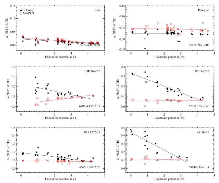
The major differences between 1D and $\langle 3\rm{D}\rangle$, as well as LTE and NLTE, are apparent from inspection of the Fe abundances in the Table 5 and the NLTE abundance corrections shown in Fig. 9. For the Sun and Procyon, the NLTE effects are rather subtle. The difference between the LTE and NLTE abundances determined from the Fe i lines is even slightly smaller in the $\langle 3\rm{D}\rangle$ case compared to 1D (Fig. 9, top panels). The basic reason is that the temperature gradient in the solar-metallicity marcs models is slightly steeper than in the $\langle 3\rm{D}\rangle$ models (Fig. 1). At $\log\tau_{\rm 5000}>0$, where the UV-blue continuum is formed, $\left(dT/d\tau\right)_{\rm 1D}>\left(dT/d\tau\right)_{\rm 3D}$, whereas in the outer layers the gradients are very similar. Over-ionization in Fe i by radiation field emerging from the hot deep layers is, thus, somewhat stronger in the marcs models.

Over-ionization is more important at low metallicities (see Sect. 3 of this paper, and a more extensive discussion in Paper II). This causes non-negligible differences between the NLTE and LTE abundances inferred from the Fe i lines. The differences are in the range $0.05-0.15$ dex for 1D models and weak Fe i lines, but increase to $0.2-0.5$ dex for the strong low-excitation Fe i lines with the $\langle 3\rm{D}\rangle$ models (Fig. 9). The larger NLTE effects of metal-poor $\langle 3\rm{D}\rangle$ models compared to 1D models are due to the larger decoupling between the radiation temperature and the local temperature, owing to the dramatically cooler outer layers of the $\langle 3\rm{D}\rangle$ models compared to 1D (see Sect. 3 and Fig. 6). NLTE corrections to the Fe ii lines are negative and are not larger than $-0.03$ dex. As a result, for the metal-poor stars, the difference between the mean LTE and NLTE Fe abundances is, at least, twice as large in the $\langle 3\rm{D}\rangle$ case compared to that obtained with marcs and mafags-os models. On the other side, the same phenomenon, which leads to amplified NLTE effects in the $\langle 3\rm{D}\rangle$ calculations, i.e., very steep $\left(dT/d\tau\right)$ above $\log\tau_{\rm 5000}\approx 0$, is also responsible for the LTE strengthening of the Fe i lines in $\langle 3\rm{D}\rangle$ compared to 1D. The Fe ii lines are only slightly weaker in $\langle 3\rm{D}\rangle$ calculations. Our LTE 1D metallicities are, thus, systematically larger than the $\langle 3\rm{D}\rangle$ results, in agreement with other studies (e.g., Collet, Asplund & Trampedach, 2007). We note, however, that direct comparison of our results with that of, e.g., Collet et al. (2007), is not meaningful since they performed LTE line formation calculations with full 3D hydrodynamic model atmospheres.

The fact that the $\langle 3\rm{D}\rangle$ models also predict somewhat lower LTE Fe abundances, yet larger NLTE abundance corrections than 1D models, has the important consequence that the mean NLTE metallicities in 1D and $\langle 3\rm{D}\rangle$ turn out to be in agreement for the whole range of stellar parameters ($\Delta\log\varepsilon_{\rm Fe}\leq 0.1$).

However, even though the mean metallicities are similar, individual Fe i line abundances are still somewhat discrepant, and show systematic trends with line equivalent width and excitation potential of the lower level of a transition, $E_{\rm low}$ (Figs. 13, 14). NLTE abundances inferred from the low-excitation lines of Fe i with 1D models are too large compared to the high-excitation lines and lines of Fe ii. A very similar picture is obtained with the LTE approximation, and it reverses sign in LTE $\langle 3\rm{D}\rangle$. A combination of $\langle 3\rm{D}\rangle$ and NLTE alleviates this discrepancy, so that Fe i and Fe ii abundances become more consistent. The improvement comes from the different sensitivity of the NLTE effects to $E_{\rm low}$ in the 1D and $\langle 3\rm{D}\rangle$ case. This is clearly seen in Fig. 9. A least-square fit to the NLTE abundance corrections is also shown, which is a simple albeit very illustrative measure of the mean NLTE effect on the excitation balance of Fe i. In the 1D case, the Fe i lines have rather similar NLTE corrections irrespective of their excitation potential and equivalent width. In the $\langle 3\rm{D}\rangle$ case, however, the low-excitation transitions, $E_{\rm low}\leq 2$ eV, tend to experience significantly larger departures from LTE compared to the higher-excitation transitions. The reason is that, owing to the dramatically cooler surfaces of the metal-poor $\langle 3\rm{D}\rangle$ models, low-excitation Fe i lines become stronger and more sensitive to the physical conditions in the outer atmospheric layers, where the influence of non-local radiation field is extreme, not only decreasing the line opacity but also pushing the line source functions to super-thermal values. Thus, the NLTE $\langle 3\rm{D}\rangle$ profiles of these lines are weaker compared to LTE. The magnitude of this effect depends on stellar parameters (see also the discussion in Sect. 3). As a consequence, one would also expect that excitation balance achieved under LTE with the $\langle 3\rm{D}\rangle$ models will strongly overestimate $T_{\mathrm{eff}}$, and the error shall increase with $T_{\mathrm{eff}}$ and decreasing metallicity as indicated by the increasing slope of $\Delta({\rm NLTE-LTE})$ vs $E_{\rm low}$ for more metal-poor and hotter stars.

A corollary is that accurate metallicities for late-type stars can be obtained with standard 1D model atmospheres if NLTE effects in Fe i are taken into account. However, this is true only if the following condition is satisfied: a sufficiently large number of Fe i and Fe ii lines of different types are included in an analysis, so that individual line-to-line abundance discrepancies cancel out. This approach, however, does not eliminate residual trends of abundance with line equivalent width and excitation potential. Although these trends can be, at least in part, corrected for by adjusting microturbulence, a better approach is to restrict an analysis with 1D hydrostatic models to high-excitation Fe i lines only, as also advocated in the literature (e.g., Gustafsson, 1983).

4.5.2 Effective temperatures and surface gravities

Figure 10: Comparison of spectroscopic stellar parameters, $T_{\mathrm{eff}}$ and $\log g$, with the data obtained by independent methods, IRFM and parallaxes. G 64-12 is not shown in the bottom figure, because its astrometric gravity is too uncertain.

The spectroscopic effective temperatures and surface gravities determined according to the procedure described in Sect. 4.1 are given in the Table 6.

Fig. 10 (top panel) plots the effective temperatures obtained for the reference stars adopting a fixed surface gravity inferred from stellar parallaxes. The results are shown for the three cases: LTE, NLTE with the standard model atom ($S\!_{\rm H}=1$), and NLTE with Drawin’s H i collision cross-sections scaled by a factor of $S\!_{\rm H}=0.1$. The reference temperature scale, T_eff,REF, refers to the IRFM results (see Sect. 4.2) for all stars but Procyon with the interferometric angular diameters; their uncertainties are shown with blue filled areas. The uncertainties of our spectroscopic $T_{\mathrm{eff}}$’s were estimated by mapping the errors in atomic transition probabilities, observational errors, and errors in the input surface gravity into a range in temperatures. In order not to overload the figures, these errors are shown for the NLTE $S\!_{\rm H}=1$ solution only. We emphasize that the $T_{\mathrm{eff}}$’s were obtained by enforcing ionization balance, but not requiring null slopes with excitation potential for the reasons discussed above.

The overall best result in terms of consistency between the spectroscopic effective temperatures, T_eff,Fe, and effective temperatures obtained by independent methods, T_eff,REF, is achieved under NLTE using the reference model atom with $S\!_{\rm H}=1$, i.e. standard Drawin’s H i collisions. The 1D and $\langle 3\rm{D}\rangle$ models perform similarly, predicting only minor offsets of T_eff,Fe from the reference IRFM $T_{\mathrm{eff}}$ scale, with an rms error of the order of $\sim 50$ K. Assuming LTE or decreasing the efficiency of inelastic H i collisions in the NLTE statistical equilibrium calculations by an order of magnitude, $S\!_{\rm H}=0.1$, leads to larger discrepancies. The latter result is very important. At low metallicity NLTE effects in Fe i are extremely sensitive to the magnitude of collisional thermalization by H i. Our analysis, thus, not only confirms that it is possible to constrain the absolute magnitude of atomic collision cross-sections using metal-poor stars, but also demonstrates that a single scaling factor (unity in our case) to the classical Drawin’s formula is a reasonable approximation. What concerns the LTE $T_{\mathrm{eff}}$ values, they are still within the errors of T_eff,REF in the 1D case. We caution, however, that the NLTE effects for our stars are small in 1D, and this statement may not apply for stellar parameters where the NLTE effects are more significant, i.e. for stars with higher $T_{\mathrm{eff}}$ and lower $\log g$. The discrepancy between the LTE spectroscopic and the IRFM scale increases to $200$ K for the metal-poor stars when $\langle 3\rm{D}\rangle$ models are employed, which is consistent with the discussion in the previous section.

Our second approach, in which the $T_{\mathrm{eff}}$ values are kept fixed and surface gravities are obtained by forcing Fe ionization equilibria, returns similar results. Fig. 10 (bottom panel) compares the spectroscopic $\log g$’s with the values determined from parallaxes, the shaded regions indicate the uncertainty of the latter (see Sect. 4.2) and the error bars of the former account for the uncertainties in $\log gf$, IRFM effective temperatures, and observational uncertainties. As seen from this figure, only the NLTE approach with $S\!_{\rm H}=1$ gives $\log g$ values on average consistent with that inferred from parallaxes. In $\langle 3\rm{D}\rangle$, LTE gravities are systematically too low. In 1D, the discrepancy is smaller, but appears to increase with $T_{\mathrm{eff}}$. The assumption of $S\!_{\rm H}=0.1$ brings the Fe i abundances so high, that much larger gravities are generally needed to match Fe i with Fe ii.

4.5.3 Comparison with other studies

Korn et al. (2003) performed a study similar to ours aiming to constrain the efficiency of inelastic H i collisions from the NLTE 1D Fe calculations for a small sample of late-type stars. Using the mafags-os model atmospheres and the Drawin’s formulae for H i collision cross-sections, they determined $S\!_{\rm H}=3$ as a scaling factor to the latter yielding satisfactory ionization balance of Fe i and Fe ii. For the stars in common, HD 140283, HD 84937, and Procyon, their results are consistent with our values for $S\!_{\rm H}=1$. This study was, however, later superseded by that of Mashonkina et al. (2011), in which the Fe model atom of Gehren et al. (2001, b), also used by Korn et al. (2003), was updated by more recent atomic data. This work, in fact, showed that a lower efficiency of inelastic H i collisions ($S\!_{\rm H}=0.1$) is needed to satisfy ionization balance of Fe. Their results for HD 84937 and HD 122563 are in agreement with our values within the error bars: $-2.00\pm 0.07$ (Fe I) respectively $-2.08\pm 0.04$ (Fe II) for HD 84937, and $-2.61\pm 0.09$ (Fe I) respectively $-2.56\pm 0.07$ (Fe II) for HD 122563. They also find that the NLTE Fe i-based abundances are correlated with line excitation potential, with a slope of $0.013$ dex eV^-1 for HD 84937 and $-0.054$ dex eV^-1 for HD 122563. From Fig. 13, we can not confirm their slope for HD 84937 with 1D models, however, we would get exactly same results, adopting Mashonkina et al. linelists. Their positive slope for HD 84937 would likely had vanished had they included few more subordinate near-UV Fe i lines with very accurate $gf$-values in their analysis. For HD 122563, however, we also find a small discrepancy between the high-excited Fe i and Fe ii lines, in addition to residual slopes of the NLTE Fe abundances with $E_{\rm low}$: $-0.11$ dex eV^-1 for the mafags-os, $-0.09$ dex eV^-1 for marcs, and $-0.05$ dex eV^-1 for the $\langle 3\rm{D}\rangle$ model. One of the important differences between our and their study, which also explains our more extreme slopes in 1D, is the way we handle microturbulence. We use Fe ii lines, whereas Mashonkina et al. (2011) rely on the Fe i lines. Nevertheless, the fact that our results obtained with 1D model atmospheres support the findings of Mashonkina et al. (2011) is reassuring.

4.5.4 HD 122563

HD 122563 is one of the most well-studied metal-poor giants. Nevertheless, its parameters are badly constrained. For example, Fulbright (2000) gives $T_{\mathrm{eff}}=4425$ K, $\log g=0.6$, and [Fe/H] $=-2.6$, whereas according to Mashonkina et al. (2011) the star is better described by a model with $T_{\mathrm{eff}}=4600$ K, $\log g=1.6$, and [Fe/H] $\approx-2.58$.

At $S\!_{\rm H}=1$, no combination of parameters can achieve a fully satisfactory spectroscopic solution for this star, consistently achieving adequate excitation and ionization balance. This is evident from the residual offset between the high-excitation Fe i and Fe ii lines in Fig. 14. In NLTE with $S\!_{\rm H}=1$, the spectroscopic $\log g$ is $0.3$ dex lower than the value derived from the Hipparcos parallax. The discrepancy can be minimized by adopting less efficient hydrogen collisions, which, however, contradicts the spectroscopic results of the other metal-poor stars.

Based on HD122563 alone, the evidence for a lower $S\!_{\rm H}$ is thus limited. Similar investigation of larger samples of metal-poor giants and dwarfs with well-defined parameters may help to better clarify the situation.

4.6 Comparison with evolutionary tracks

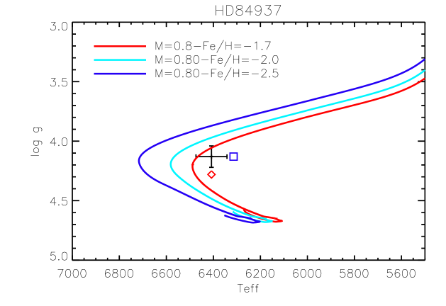
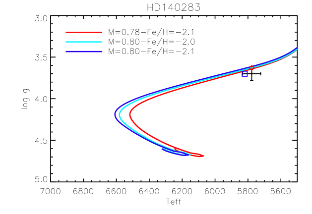
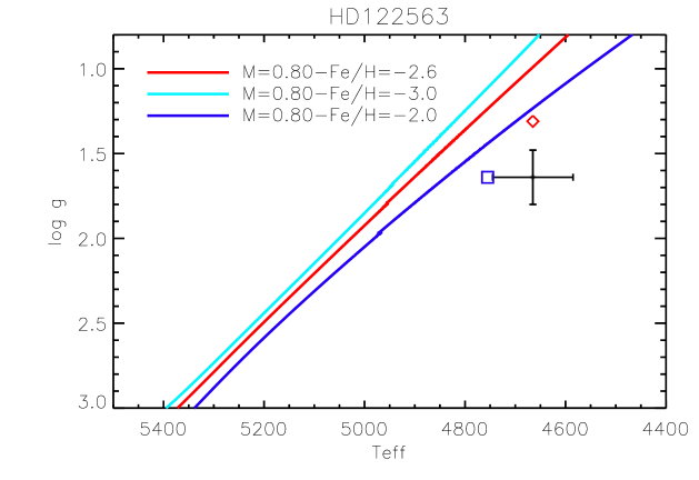
In an attempt to assess the trustworthiness of the spectroscopic results versus those obtained from independent measurements, we compared them to evolutionary tracks. The position of the four metal-poor stars in the $T_{\mathrm{eff}}$-$\log g$ plane is shown in Fig. 11. The black cross with error bars indicated is the result with the IRFM $T_{\mathrm{eff}}$ and astrometric surface gravity, and the blue square and red diamond correspond to our spectroscopic $\langle 3\rm{D}\rangle$ NLTE $T_{\mathrm{eff}}$ and $\log g$, respectively. For comparison, evolutionary tracks with close parameters computed with the garstec code (Weiss & Schlattl, 2008) are shown. These were kindly made available to us by A. Serenelli (2011, private communication). In order not to overload the figures, we show only the NLTE $\langle 3\rm{D}\rangle$ spectroscopic results, while briefly discussing other solutions from the Table 6 below.

For all metal-poor stars, a combination of astrometric gravity and spectroscopic $T_{\mathrm{eff}}$/[Fe/H], obtained with NLTE $S\!_{\rm H}=1$ or LTE with 1D and $\langle 3\rm{D}\rangle$ models, appears to be most consistent with stellar evolution calculations. The error bars of our data are omitted in the plots for clarity (they are given in the Table 6). 1D LTE $T_{\mathrm{eff}}$’s are somewhat larger than the 1D NLTE results, that makes the stars a bit more massive. It is interesting that even with $\langle 3\rm{D}\rangle$ LTE effective temperatures, which are $\sim 50-300$ K larger compared to NLTE results, the stars still match the tracks with adequate mass and metallicity, which, in fact, also implies more realistic ages.

A combination of IRFM $T_{\mathrm{eff}}$ and the spectroscopic $\langle 3\rm{D}\rangle$ LTE $\log g$/[Fe/H] makes the agreement with stellar evolution less satisfactory. In particular, HD 140283 is now in the ’forbidden’ zone of the HRD. Situation is even worse for the NLTE $S\!_{\rm H}=0.1$ results, obtained with 1D and with $\langle 3\rm{D}\rangle$ model atmospheres. In this case, all four metal-poor stars are some $\sim 2-3\sigma$ in $T_{\mathrm{eff}}$ and $\log g$ away from any reasonable track.

HD 122563 is a somewhat outstanding object. Assuming the tracks to be realistic, it also becomes clear that the IRFM $T_{\mathrm{eff}}$ and/or luminosity of the star inferred from its relatively accurate parallax are too low. Other attempts, such as variation of the mass or decreasing the $\alpha$-enhancement, either do not have any effect or make the discrepancy with masses and ages even larger. In this respect, it is encouraging that our spectroscopic $\langle 3\rm{D}\rangle$ NLTE values of $T_{\mathrm{eff}}$ and $\log g$ bring the star into a much better agreement with stellar evolution, although these value appear to be shifted away from the presumably more reliable IRFM temperature and astrometric gravity.

Figure 11: The position of the four metal-poor stars in the $T_{\mathrm{eff}}$-$\log g$ plane. The black cross with error bars is the result with the IRFM $T_{\mathrm{eff}}$ and astrometric surface gravity, and the blue square and red diamond correspond to the spectroscopic NLTE $\langle 3\rm{D}\rangle$ $T_{\mathrm{eff}}$ and $\log g$ from this work, respectively. garstec evolutionary tracks are also shown for comparison. For G 64-12 only spectroscopic $\log g$/IRFM $T_{\mathrm{eff}}$ solution is shown.

5 Summary and conclusions

One important problem in spectroscopy of late-type stars is to quantify systematic errrors in the determination of $T_{\mathrm{eff}}$, $\log g$, and [Fe/H] from the Fe i/Fe ii excitation-ionization equilibrium due to the assumptions of LTE and hydrostatic equilibrium in the models.

We have constructed a new extensive NLTE Fe model atom using the most up-to-date theoretical and experimental atomic data available so far. The model has been applied to the analysis of the Sun and a number of well-studied late-type stars with parameters determined by other independent methods. We have used standard 1D LTE marcs and mafags-os model atmospheres, as well as average stratifications computed from full time-dependent, 3D, hydrodynamical simulations of stellar surface convection. In addition, we compared the commonly-used NLTE line formation program packages detail/siu and multi. Despite obvious differences in their numerical scheme and input physical data, we find that the final results are consistent both in terms of the NLTE statistical equilibria and absolute LTE and NLTE abundances.

Our LTE and NLTE results for the 1D models are similar to most of the previous findings in the literature. Statistical equilibrium of Fe, which is a minority ion at the typical conditions of these cool and dense atmospheres, favors lower number densities of Fe i compared to LTE. The number densities of Fe ii are hardly affected by NLTE. In general, this leads to a weakening of Fe i lines compared to LTE, which, in turn, requires larger Fe abundance to fit a given observed spectral line. The magnitude of departures from LTE depends on stellar parameters. With 1D hydrostatic model atmospheres the NLTE corrections on Fe i lines do not exceed $0.1$ dex for stars with [Fe/H] $>-3.5$, and they are negligible for the Fe ii lines. The situation changes dramatically for the mean 3D ($\langle 3\rm{D}\rangle$) models with their cooler surfaces, and, thus, steeper T$(\tau)$ relations. The NLTE abundance corrections can be as large as $\sim 0.5$ dex for the resonance Fe i lines formed in very metal-poor atmospheres. In contrast to LTE, NLTE strengths of the Fe i lines predicted by the $\langle 3\rm{D}\rangle$ and 1D models are rather similar, because the line formation is largely dictated by the radiation field forming around the optical surface, $\log\tau_{\rm 5000}\sim 0$, where the thermal structures of $\langle 3\rm{D}\rangle$ and 1D models are similar. This suggests that the full 3D NLTE results, once they become feasible, will be even closer to our $\langle 3\rm{D}\rangle$ NLTE calculations.

The solar Fe abundance obtained under NLTE using the $\langle 3\rm{D}\rangle$ model atmospheres is $7.46\pm 0.06$ dex, and the uncertainty is fully dominated by the errors of the experimental transition probabilities. Adopting LTE or 1D hydrostatic model atmospheres lowers the solar Fe abundance by $\sim 0.02$ dex. For Procyon we infer slightly sub-solar metallicity, [Fe/H] $=-0.03$ dex.

We find that the Fe i/Fe ii ionization balance can be well established for all reference stars with the 1D and $\langle 3\rm{D}\rangle$ model atmospheres and the NLTE model atom with Drawin’s H i collision cross-sections. Strong resonance and subordinate Fe i lines are very sensitive to the atmospheric structure, thus, classical 1D models fail to provide consistent excitation balance. A better agreement among Fe i lines spanning a range of excitation potential is obtained with the mean 3D models, although the optimum solution, which fully eliminates the correlation of the abundance and line excitation potential, may necessitate self-consistent NLTE modelling with full 3D hydrodynamical model atmospheres. The assumption of LTE in combination with $\langle 3\rm{D}\rangle$ models leads to large errors in $T_{\mathrm{eff}}$ and $\log g$ inferred from the Fe ionization balance, yet we find satisfactory results for certain combinations of stellar parameters using standard hydrostatic model atmospheres.

The mean NLTE metallicities determined with 1D and $\langle 3\rm{D}\rangle$ models are in agreement in the range of stellar parameters investigated here, although there are marked residual slopes of abundance with line excitation potential and strength. We can, thus, conclude that accurate, albeit not precise, metallicities for late-type stars can be obtained with classical hydrostatic 1D model atmospheres if NLTE effects in Fe i are taken into account and a sufficiently large number of Fe i and Fe ii lines with different excitation potentials is used, so that individual line-to-line abundance discrepancies cancel out. An alternative solution, which avoids additional biases introduced by adjusting microturbulence parameter, is to use high-excitation Fe i lines only. Thus, the results obtained with classical 1D models depend on the choice of the line list and, in particular, on the balance of the number of lines of different types. A combination of $\langle 3\rm{D}\rangle$ and NLTE alleviates this problem.

Our NLTE effective temperatures and gravities are consistent with the parameters determined by other less model-dependent methods, in particular with IRFM $T_{\mathrm{eff}}$’s and $\log g$’s inferred from parallaxes. The results for the metal- poor dwarfs and subgiant are also consistent with stellar evolution predictions. For HD 122563, the results are inconclusive. In addition to a residual slope of Fe i-based abundances with line excitation potential, the NLTE $\langle 3\rm{D}\rangle$ spectroscopic gravity is roughly $0.3$ dex lower than the astrometric result. On the one side, the latter is somewhat uncertain due to the difficulty of determining the mass of this metal-poor giant. Furthermore, comparisons with evolutionary tracks favor higher $T_{\mathrm{eff}}$ and lower $\log g$ which would be more consistent with our spectroscopic estimates. On the other side, the discrepancies might be indicative of remaining systematic uncertainties in the stellar atmosphere models, such as neglect of convective inhomogeneities and atmospheric extension, which become increasingly important with increasing $T_{\mathrm{eff}}$ and decreasing $\log g$. The importance of the latter is also amplified at higher metallicities.

Figure 12: NLTE abundances determined from the low-excitation Fe i (filled circles), high-excited Fe i (blue diamonds), and Fe ii (squares) lines using marcs-os, mafags-os, and $\langle 3\rm{D}\rangle$ model atmospheres for the Sun (top) and Procyon (bottom). Small vertical bars on the left and right-hand side of each plot show the size of NLTE abundance corrections for the low-excited ($<2.5$ eV) and high-excited Fe i lines, respectively. They are leveled out at the mean NLTE abundance obtained from the Fe i and Fe ii lines with $S\!_{\rm H}=1$. The bar’s upper and lower ends correspond to the mean NLTE abundance obtained with $S\!_{\rm H}=0.1$ and the LTE abundance, respectively. The dark and light shaded regions indicate the standard and total errors of the mean (see text).

Figure 13: Abundances determined from the Fe I and Fe II lines using stellar parameters from Table 5 for HD 84937 (top) and HD 140283 (bottom).

Figure 14: Abundances determined from the Fe I and Fe II lines using stellar parameters from Table 5 for HD 122563 (top) and G 64-12 (bottom). Note that the total errors are large as they also reflect the uncertainties in the input stellar parameters.

Table 8: Equivalent widths of the Fe i lines (in units of mÅ).

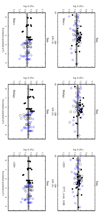
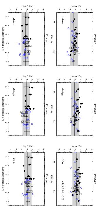
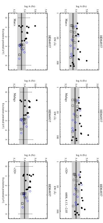
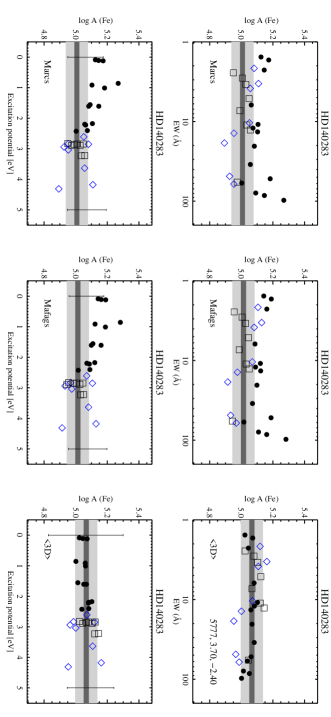
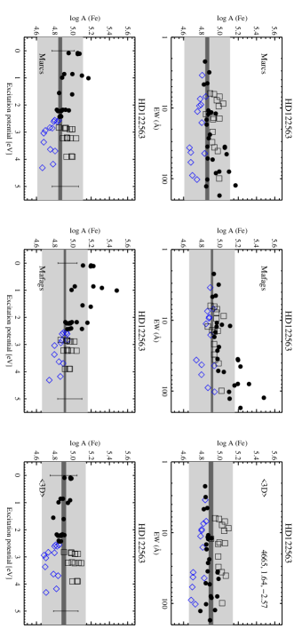
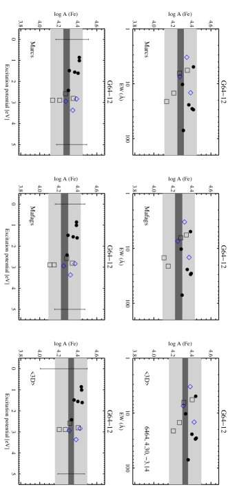
Line (Å)	Sun	Procyon	HD 84937	HD 140283	HD 122563	G 64-12
3581.19			136.30			90.00
3618.77			100.95			61.80
3719.93						89.00
3737.13						80.60
3745.56						71.35
3758.23						64.00
3820.43			138.90			70.40
4045.81			115.95			71.02
4235.94			52.55	59.23	102.58	10.30
4250.79			71.90	78.99	128.14	24.26
4415.12			75.30	84.90		28.59
4445.47	41.05	8.49			12.02
4494.56	204.79	123.69	28.94	34.62	83.36
4920.50	522.83	207.10	55.68	61.03	102.54	14.60
4994.13	111.49	87.12	7.33	13.49	79.57
5044.21	77.48	48.67		2.15	9.35
5198.71	101.08	75.32	4.25	6.20	35.22
5216.27	129.41	99.89	13.90	20.41	79.26
5225.53	73.14	32.95		2.26	45.02
5232.94	389.77	180.23	44.80	48.73	89.72	7.40
5236.20	34.77	16.93
5242.49	90.82	72.53	3.42	3.84	11.22
5247.05	67.15	25.53		1.55	36.52
5250.21	66.95	25.64		1.69	35.45
5269.54	533.08	204.43	84.46	97.47	172.99	29.70
5281.79	164.04	104.41	11.93	14.03	42.52
5379.57	60.26	38.82			3.45
5383.37	229.36	132.15	20.96	18.62	36.45
5434.52	213.36	130.93	37.18	52.31	124.32	4.94
5491.84	14.23	4.91
5586.76			26.01		58.67	3.30
5661.35	24.87	10.25
5662.52	102.45	75.49		3.34	7.44
5701.54	86.97	57.59			16.14
5705.46	39.97	21.17
5916.25	54.06	24.82
5956.69	52.47	16.22			11.56
6065.48	131.32	93.35	8.48	10.40	43.92
6082.71	34.67	9.75			2.21
6151.62	50.17	19.41			4.66
6173.33	68.47	36.51			10.86
6200.31	73.66	44.14			9.00
6219.28	90.55	63.29	2.60		26.80
6240.65	48.75	18.63			4.49
6252.56	133.16	93.79	8.26	12.09	51.82
6265.13	88.59	57.68			23.83
6297.79	76.07	45.84			14.69
6430.85	119.06	90.63	7.09	10.88	53.67
6518.37	58.16	29.10
6574.23	28.80				3.14
6593.87	86.59	53.43			17.17
6609.11	65.27	32.12			6.90
6699.14	8.96
6726.67	49.91	27.36
6739.52	12.08
6750.15	75.95	44.28			12.29
6793.26	13.81
6810.26	52.15	30.02
6837.01	17.92
6854.82	12.28
6945.20	83.35	54.60
6978.85	80.56	50.56
7401.68	43.41	22.22
7912.87	46.89
8293.51	60.14

Table 9: Equivalent widths of the Fe ii lines (in units of mÅ).

Line (Å)	Sun	Procyon	HD 84937	HD 140283	HD 122563	G 64-12
4233.17						6.40
4491.40	76.77	104.32	9.02	7.32	30.49
4508.29
4576.34	68.55	93.19	5.96	5.16	21.74
4582.84	56.51	80.64	3.38	2.85	14.46
4583.84						5.70
4620.52	53.91	75.55	3.16	2.45	12.24
4923.93	190.40		62.07	57.67	99.18	14.85
5169.03						21.10
5197.58	85.22	115.09	13.08	11.07	36.14
5234.62	84.37	122.16	15.35	12.77	40.63
5264.81	47.81	69.23			8.68
5284.11	62.01	87.00	3.90	3.42
5325.55	44.71	66.42			6.23
5414.07	28.83	44.12
5425.26	43.50	63.26			6.39
6239.95	13.18	25.00
6247.56	56.21	83.62	3.22		9.44
6369.46	19.75	29.78
6432.68	41.16	62.63			7.80
6456.38	66.79	98.26	5.48		13.74
6516.08	56.09	75.98			14.12
7222.39	19.35	35.36
7515.83	15.16	27.30
7711.72	49.09				6.94

References

- Allen (1973) Allen C. W., 1973, Astrophysical quantities. London: University of London, Athlone Press, 1973, 3rd ed.
- Asplund et al. (2009) Asplund M., Grevesse N., Sauval A. J., Scott P., 2009, ARAA, 47, 481
- Asplund et al. (2000) Asplund M., Nordlund Å., Trampedach R., Allende Prieto C., Stein R. F., 2000, A&A, 359, 729
- Asplund et al. (1999) Asplund M., Nordlund Å., Trampedach R., Stein R. F., 1999, A&A, 346, L17
- Athay & Lites (1972) Athay R. G., Lites B. W., 1972, ApJ, 176, 809
- Auer (1987) Auer L. H., 1987, Acceleration of Convergence. Cambridge: University Press
- Aufdenberg et al. (2005) Aufdenberg J. P., Ludwig H.-G., Kervella P., 2005, ApJ, 633, 424
- Bagnulo et al. (2003) Bagnulo S., Jehin E., Ledoux C., Cabanac R., Melo C., Gilmozzi R., The ESO Paranal Science Operations Team 2003, The Messenger, 114, 10
- Bard et al. (1991) Bard A., Kock A., Kock M., 1991, A&A, 248, 315
- Bard & Kock (1994) Bard A., Kock M., 1994, A&A, 282, 1014
- Barklem & Aspelund-Johansson (2005) Barklem P. S., Aspelund-Johansson J., 2005, A&A, 435, 373
- Barklem et al. (2011) Barklem P. S., Belyaev A. K., Guitou M., Feautrier N., Gadéa F. X., Spielfiedel A., 2011, A&A, 530, A94
- Barklem et al. (2000) Barklem P. S., Piskunov N., O’Mara B. J., 2000, VizieR Online Data Catalog, 414, 20467
- Bautista (1997) Bautista M. A., 1997, A&AS, 122, 167
- Bernkopf (1998) Bernkopf J., 1998, A&A, 332, 127
- Bikmaev et al. (1990) Bikmaev I. F., Bobritskii S. S., Sakhibullin N. A., 1990, Soviet Astronomy Letters, 16, 91
- Blackwell et al. (1986) Blackwell D. E., Booth A. J., Haddock D. J., Petford A. D., Leggett S. K., 1986, MNRAS, 220, 549
- Blackwell et al. (1979) Blackwell D. E., Ibbetson P. A., Petford A. D., Shallis M. J., 1979, MNRAS, 186, 633
- Blackwell et al. (1979) Blackwell D. E., Petford A. D., Shallis M. J., 1979, MNRAS, 186, 657
- Blackwell et al. (1980) Blackwell D. E., Petford A. D., Shallis M. J., Simmons G. J., 1980, MNRAS, 191, 445
- Blackwell et al. (1982) Blackwell D. E., Petford A. D., Shallis M. J., Simmons G. J., 1982, MNRAS, 199, 43
- Blackwell et al. (1982) Blackwell D. E., Petford A. D., Simmons G. J., 1982, MNRAS, 201, 595
- Blackwell & Shallis (1979) Blackwell D. E., Shallis M. J., 1979, MNRAS, 186, 673
- Blackwell et al. (1982) Blackwell D. E., Shallis M. J., Simmons G. J., 1982, MNRAS, 199, 33
- Butler & Giddings (1985) Butler K., Giddings J., 1985, Newsletter on Analysis of Astronomical Spectra, University of London, 9
- Canuto & Mazzitelli (1991) Canuto V. M., Mazzitelli I., 1991, ApJ, 370, 295
- Carlsson (1986) Carlsson M., 1986, Uppsala Astronomical Observatory Reports, 33
- Carlsson (1992) Carlsson M., 1992, in M. S. Giampapa & J. A. Bookbinder ed., Cool Stars, Stellar Systems, and the Sun Vol. 26 of Astronomical Society of the Pacific Conference Series, The MULTI Non-LTE Program (Invited Review). p. 499
- Casagrande et al. (2010) Casagrande L., Ramírez I., Meléndez J., Bessell M., Asplund M., 2010, A&A, 512, A54+
- Collet et al. (2005) Collet R., Asplund M., Thévenin F., 2005, A&A, 442, 643
- Collet et al. (2007) Collet R., Asplund M., Trampedach R., 2007, A&A, 469, 687
- Collet et al. (2011) Collet R., Magic Z., Asplund M., 2011, Journal of Physics Conference Series, 328, 012003
- Cram et al. (1980) Cram L. E., Lites B. W., Rutten R. J., 1980, ApJ, 241, 374
- Fabbian et al. (2009) Fabbian D., Nissen P. E., Asplund M., Pettini M., Akerman C., 2009, A&A, 500, 1143
- Freytag et al. (1999) Freytag B., Ludwig H.-G., Steffen M., 1999, in A. Gimenez, E. F. Guinan, & B. Montesinos ed., Stellar Structure: Theory and Test of Connective Energy Transport Vol. 173 of Astronomical Society of the Pacific Conference Series, A Calibration of the Mixing-Length for Solar-Type Stars Based on Hydrodynamical Models of Stellar Surface Convection. p. 225
- Gehren et al. (2001) Gehren T., Butler K., Mashonkina L., Reetz J., Shi J., 2001, A&A, 366, 981
- Gehren et al. (2001) Gehren T., Korn A. J., Shi J., 2001, A&A, 380, 645
- Gehren et al. (2004) Gehren T., Liang Y. C., Shi J. R., Zhang H. W.and Zhao G., 2004, A&A, 413, 1045
- Gehren et al. (2006) Gehren T., Shi J. R., Zhang H. W., Zhao G., Korn A. J., 2006, A&A, 451, 1065
- Grevesse & Sauval (1999) Grevesse N., Sauval A. J., 1999, A&A, 347, 348
- Grupp (2004a) Grupp F., 2004a, A&A, 420, 289
- Grupp (2004b) Grupp F., 2004b, A&A, 426, 309
- Grupp et al. (2009) Grupp F., Kurucz R. L., Tan K., 2009, A&A, 503, 177
- Gustafsson (1983) Gustafsson B., 1983, Publications of the Astronomical Society of the Pacific, 95, 101
- Gustafsson et al. (2008) Gustafsson B., Edvardsson B., Eriksson K., Jørgensen U. G., Nordlund Å., Plez B., 2008, A&A, 486, 951
- Henyey et al. (1965) Henyey L., Vardya M. S., Bodenheimer P., 1965, ApJ, 142, 841
- Lind et al. (2012) Lind K., Bergemann M., Asplund M., 2012, MNRAS
- Martin et al. (1988) Martin G. A., Fuhr J. R., Wiese W. L., 1988, Atomic transition probabilities. Scandium through Manganese. New York: American Institute of Physics (AIP) and American Chemical Society
- Mashonkina (2011) Mashonkina L., 2011, in Magnetic Stars Non-LTE Line Formation for Fe I and Fe II in the Atmospheres of A-F Type Stars. pp 314–321
- Mashonkina et al. (2011) Mashonkina L., Gehren T., Shi J.-R., Korn A. J., Grupp F., 2011, A&A, 528, A87
- Meléndez & Barbuy (2009) Meléndez J., Barbuy B., 2009, A&A, 497, 611
- Mihalas & Athay (1973) Mihalas D., Athay R. G., 1973, ARAA, 11, 187
- Ng (1974) Ng K.-C., 1974, Journal of Chemical Physics, 61, 2680
- Nissen et al. (2007) Nissen P. E., Akerman C., Asplund M., Fabbian D., Kerber F., Kaufl H. U., Pettini M., 2007, A&A, 469, 319
- Nissen et al. (2004) Nissen P. E., Chen Y. Q., Asplund M., Pettini M., 2004, A&A, 415, 993
-
Nordlund &
Galsgaard (1995)
Nordlund Å., Galsgaard K., 1995, Technical report, A 3D MHD code for
Parallel Computers,
http://www.astro.ku.dk/~kg/Papers/MHD_code.ps.gz. Niels Bohr Institute, University of Copenhagen - Nordlund et al. (2009) Nordlund Å., Stein R. F., Asplund M., 2009, Living Reviews in Solar Physics, 6, 2
- O’Brian et al. (1991) O’Brian T. R., Wickliffe M. E., Lawler J. E., Whaling W., Brault J. W., 1991, Journal of the Optical Society of America B Optical Physics, 8, 1185
- Olson et al. (1986) Olson G. L., Auer L. H., Buchler J. R., 1986, Journal of Quantitative Spectroscopy and Radiative Transfer, 35, 431
- Raassen & Uylings (1998) Raassen A. J. J., Uylings P. H. M., 1998, A&A, 340, 300
- Ralchenko et al. (2012) Ralchenko Y., Kramida A., Reader J., Team N. A., 2012, [Online], National Institute of Standards and Technology, Gaithersburg, MD
- Reetz (1999) Reetz J. K., 1999, Sauerstoff in kühlen Sternen und die chemische Entwicklung der Galaxis. LMU München
- Rybicki & Hummer (1991) Rybicki G. B., Hummer D. G., 1991, A&A, 245, 171
- Rybicki & Hummer (1992) Rybicki G. B., Hummer D. G., 1992, A&A, 262, 209
- Scharmer & Carlsson (1985) Scharmer G. B., Carlsson M., 1985, Journal of Computational Physics, 59, 56
- Schnabel et al. (1999) Schnabel R., Kock M., Holweger H., 1999, A&A, 342, 610
- Schnabel et al. (2004) Schnabel R., Schultz-Johanning M., Kock M., 2004, A&A, 414, 1169
- Seaton (1962) Seaton M. J., 1962, in Bates D. R., ed., Atomic and Molecular Processes The Theory of Excitation and Ionization by Electron Impact. p. 375
- Steenbock & Holweger (1984) Steenbock W., Holweger H., 1984, A&A, 130, 319
- Takeda (1994) Takeda Y., 1994, Publications of the Astronomical Society of Japan, 46, 53
- Thévenin & Idiart (1999) Thévenin F., Idiart T. P., 1999, ApJ, 521, 753
- Unsold (1955) Unsold A., 1955, Physik der Sternatmospharen, mit besonderer Berucksichtigung der Sonne.
- van Leeuwen (2007) van Leeuwen F., 2007, A&A, 474, 653
- van Regemorter (1962) van Regemorter H., 1962, ApJ, 136, 906
- VandenBerg et al. (2000) VandenBerg D. A., Swenson F. J., Rogers F. J., Iglesias C. A., Alexander D. R., 2000, ApJ, 532, 430
- Weiss & Schlattl (2008) Weiss A., Schlattl H., 2008, Astrophysics and Space Science, 316, 99
- Wijbenga & Zwaan (1972) Wijbenga J. W., Zwaan C., 1972, Sol. Phys., 23, 265