Semiparametric stationarity tests based on adaptive multidimensional increment ratio statistics

Jean-Marc Bardet and Béchir Dola

bardet@univ-paris1.fr,   bechir.dola@malix.univ-paris1.fr
 
SAMM, Université Panthéon-Sorbonne (Paris I), 90 rue de Tolbiac, 75013 Paris, FRANCE
Abstract

In this paper, we show that the adaptive multidimensional increment ratio estimator of the long range memory parameter defined in Bardet and Dola (2012) satisfies a central limit theorem (CLT in the sequel) for a large semiparametric class of Gaussian fractionally integrated processes with memory parameter d(0.5,1.25)𝑑0.51.25d\in(-0.5,1.25). Since the asymptotic variance of this CLT can be computed, tests of stationarity or nonstationarity distinguishing the assumptions d<0.5𝑑0.5d<0.5 and d0.5𝑑0.5d\geq 0.5 are constructed. These tests are also consistent tests of unit root. Simulations done on a large benchmark of short memory, long memory and non stationary processes show the accuracy of the tests with respect to other usual stationarity or nonstationarity tests (LMC, V/S, ADF and PP tests). Finally, the estimator and tests are applied to log-returns of famous economic data and to their absolute value power laws.

Keywords: Gaussian fractionally integrated processes; Adaptive semiparametric estimators of the memeory parameter; test of long-memory; stationarity test; unit root test.


1 Introduction

Consider the set I(d)𝐼𝑑I(d) of fractionally integrated time series X=(Xk)k𝑋subscriptsubscript𝑋𝑘𝑘X=(X_{k})_{k\in\mathbb{Z}} for 0.5<d<1.50.5𝑑1.5-0.5<d<1.5 by:
 
Assumption I(d)𝐼𝑑I(d): X=(Xt)t𝑋subscriptsubscript𝑋𝑡𝑡X=(X_{t})_{t\in\mathbb{Z}} is a time series if there exists a continuous function f:[π,π][0,[f^{*}:[-\pi,\pi]\to[0,\infty[ satisfying:

  1. 1.

    if 0.5<d<0.50.5𝑑0.5-0.5<d<0.5, X𝑋X is a stationary process having a spectral density f𝑓f satisfying

    f(λ)=|λ|2df(λ)for all λ(π,0)(0,π), with f(0)>0.𝑓𝜆superscript𝜆2𝑑superscript𝑓𝜆for all λ(π,0)(0,π), with f(0)>0\displaystyle f(\lambda)=|\lambda|^{-2d}f^{*}(\lambda)\quad\mbox{for all $\lambda\in(-\pi,0)\cup(0,\pi)$, with $f^{*}(0)>0$}. (1.1)
  2. 2.

    if 0.5d<1.50.5𝑑1.50.5\leq d<1.5, U=(Ut)t=XtXt1𝑈subscriptsubscript𝑈𝑡𝑡subscript𝑋𝑡subscript𝑋𝑡1U=(U_{t})_{t\in\mathbb{Z}}=X_{t}-X_{t-1} is a stationary process having a spectral density f𝑓f satisfying

    f(λ)=|λ|22df(λ)for all λ(π,0)(0,π), with f(0)>0.𝑓𝜆superscript𝜆22𝑑superscript𝑓𝜆for all λ(π,0)(0,π), with f(0)>0\displaystyle f(\lambda)=|\lambda|^{2-2d}f^{*}(\lambda)\quad\mbox{for all $\lambda\in(-\pi,0)\cup(0,\pi)$, with $f^{*}(0)>0$}. (1.2)

The case d(0,0.5)𝑑00.5d\in(0,0.5) is the case of long-memory processes, while short-memory processes are considered when 0.5<d00.5𝑑0-0.5<d\leq 0 and nonstationary processes when d0.5𝑑0.5d\geq 0.5. ARFIMA(p,d,q)𝑝𝑑𝑞(p,d,q) processes (which are linear processes) or fractional Gaussian noises (with parameter H=d+1/2(0,1)𝐻𝑑1201H=d+1/2\in(0,1)) are famous examples of processes satisfying Assumption I(d)𝐼𝑑I(d). The purpose of this paper is twofold: firstly, we establish the consistency of an adaptive semiparametric estimator of d𝑑d for any d(0.5,1.25)𝑑0.51.25d\in(-0.5,1.25). Secondly, we use this estimator for building new semiparametric stationary tests.
Numerous articles have been devoted to estimate d𝑑d in the case d(0.5,0.5)𝑑0.50.5d\in(-0.5,0.5). The books of Beran (1994) or Doukhan et al. (2003) provide large surveys of such parametric (mainly maximum likelihood or Whittle estimators) or semiparametric estimators (mainly local Whittle, log-periodogram or wavelet based estimators). Here we will restrict our discussion to the case of semiparametric estimators that are best suited to address the general case of processes satisfying Assumption I(d)𝐼𝑑I(d). Even if first versions of local Whittle, log-periodogramm and wavelet based estimators (see for instance Robinson, 1995a and 1995b, Abry and Veitch, 1998) are only considered in the case d<0.5𝑑0.5d<0.5, new extensions have been provided for also estimating d𝑑d when d0.5𝑑0.5d\geq 0.5 (see for instance Hurvich and Ray, 1995, Velasco, 1999a, Velasco and Robinson, 2000, Moulines and Soulier, 2003, Shimotsu and Phillips, 2005, Giraitis et al., 2003, 2006, Abadir et al., 2007 or Moulines et al., 2007). Moreover, adaptive versions of these estimators have also been defined for avoiding any trimming or bandwidth parameters generally required by these methods (see for instance Giraitis et al., 2000, Moulines and Soulier, 2003, or Veitch et al., 2003, or Bardet et al., 2008). However there still no exists an adaptive estimator of d𝑑d satisfying a central limit theorem (for providing confidence intervals or tests) and valid for d<0.5𝑑0.5d<0.5 but also for d0.5𝑑0.5d\geq 0.5. This is the first objective of this paper and it will be achieved using multidimensional Increment Ratio (IR) statistics.
Indeed, Surgailis et al. (2008) first defined the statistic IRN𝐼subscript𝑅𝑁IR_{N} (see its definition in (2.3)) from an observed trajectory (X1,,XN)subscript𝑋1subscript𝑋𝑁(X_{1},\ldots,X_{N}). Its asymptotic behavior is studied and a central limit theorem (CLT in the sequel) is established for d(0.5,0.5)(0.5,1.25)𝑑0.50.50.51.25d\in(-0.5,0.5)\cup(0.5,1.25) inducing a CLT. Therefore, the estimator d^N=Λ01(IRN)subscript^𝑑𝑁superscriptsubscriptΛ01𝐼subscript𝑅𝑁\widehat{d}_{N}=\Lambda_{0}^{-1}(IR_{N}), where dΛ0(d)maps-to𝑑subscriptΛ0𝑑d\mapsto\Lambda_{0}(d) is a smooth and increasing function, is a consistent estimator of d𝑑d satisfying also a CLT (see more details below). However this new estimator was not totally satisfying: firstly, it requires the knowledge of the second order behavior of the spectral density that is clearly unknown in practice. Secondly, its numerical accuracy is interesting but clearly less than the one of local Whittle or log-periodogram estimators. As a consequence, in Bardet and Dola (2012), we built an adaptive multidimensional IR𝐼𝑅IR estimator d~NIRsuperscriptsubscript~𝑑𝑁𝐼𝑅\widetilde{d}_{N}^{IR} (see its definition in (3.2)) answering to both these points but only for 0.5<d<0.50.5𝑑0.5-0.5<d<0.5. This is an adaptive semiparametric estimator of d𝑑d and its numerical performances are often better than the ones of local Whittle or log-periodogram estimators.
Here we extend this preliminary work to the case 0.5d<1.250.5𝑑1.250.5\leq d<1.25. Hence we obtain a CLT satisfied by d~NIRsuperscriptsubscript~𝑑𝑁𝐼𝑅\widetilde{d}_{N}^{IR} for all d(0.5,1.25)𝑑0.51.25d\in(-0.5,1.25) with an explicit asymptotic variance depending only on d𝑑d and this notably allows to obtain confidence intervals. The case d=0.5𝑑0.5d=0.5 is now studied and this offers new interesting perspectives: our adaptive estimator can be used for building a stationarity (or nonstationarity) test since 0.50.50.5 is the “border number” between stationarity and nonstationarity.  

There exist several famous stationarity (or nonstationarity) tests. For stationarity tests we may cite the KPSS (Kwiotowski, Phillips, Schmidt, Shin) test (see for instance Hamilton, 1994, p. 514) and LMC test (see Leybourne and McCabe, 2000). For nonstationarity tests we may cite the Augmented Dickey-Fuller test (ADF test in the sequel, see Hamilton, 1994, p. 516-528) and the Philipps and Perron test (PP test in the sequel, see for instance Elder, 2001, p. 137-146). All these tests are unit root tests, i.e. and roughly speaking, semiparametric tests based on the model Xt=ρXt1+εtsubscript𝑋𝑡𝜌subscript𝑋𝑡1subscript𝜀𝑡X_{t}=\rho\,X_{t-1}+\varepsilon_{t} with |ρ|1𝜌1|\rho|\leq 1. A test about d=0.5𝑑0.5d=0.5 for a process satisfying Assumption I(d)𝐼𝑑I(d) is therefore a refinement of a basic unit root test since the case ρ=1𝜌1\rho=1 is a particular case of I(1)𝐼1I(1) and the case |ρ|<1𝜌1|\rho|<1 a particular case of I(0)𝐼0I(0). Thus, a stationarity (or nonstationarity test) based on the estimator of d𝑑d provides a more sensible test than usual unit root tests.
This principle of stationarity test linked to d𝑑d was also already investigated in many articles. We can notably cite Robinson (1994), Tanaka (1999), Ling and Li (2001), Ling (2003) or Nielsen (2004). However, all these papers provide parametric tests, with a specified model (for instance ARFIMA or ARFIMA-GARCH processes). More recently, several papers have been devoted to the construction of semi-parametric tests, see for in instance Giraitis et al. (2006), Abadir et al. (2007) or Surgailis et al. (2006).
Here we slightly restrict the general class I(d)𝐼𝑑I(d) to the Gaussian semiparametric class IG(d,β)𝐼𝐺𝑑𝛽IG(d,\beta) defined below (see the beginning of Section 2). For processes belonging to this class, we construct a new stationarity test S~Nsubscript~𝑆𝑁\widetilde{S}_{N} which accepts the stationarity assumption when d~NIR0.5+ssuperscriptsubscript~𝑑𝑁𝐼𝑅0.5𝑠\widetilde{d}_{N}^{IR}\leq 0.5+s with s𝑠s a threshold depending on the type I error test and N𝑁N, while the new nonstationarity test T~Nsubscript~𝑇𝑁\widetilde{T}_{N} accepts the nonstationarity assumption when d~NIR0.5ssuperscriptsubscript~𝑑𝑁𝐼𝑅0.5𝑠\widetilde{d}_{N}^{IR}\geq 0.5-s. Note that d~NIRssuperscriptsubscript~𝑑𝑁𝐼𝑅superscript𝑠\widetilde{d}_{N}^{IR}\leq s^{\prime} also provides a test for deciding between short and long range dependency, as this is done by the V/S test (see details in Giraitis et al., 2003)
 
In Section 5, numerous simulations are realized on several models of time series (short and long memory processes).
First, the new multidimensional IR estimator d~NIRsuperscriptsubscript~𝑑𝑁𝐼𝑅\widetilde{d}_{N}^{IR} is compared to the most efficient and famous semiparametric estimators for d[0.4,1.2]𝑑0.41.2d\in[-0.4,1.2]; the performances of d~NIRsuperscriptsubscript~𝑑𝑁𝐼𝑅\widetilde{d}_{N}^{IR} are convincing and equivalent to close to other adaptive estimators (except for extended local Whittle estimator defined in Abadir et al., 2007, which provides the best results but is not an adative estimator).
Secondly, the new stationarity S~Nsubscript~𝑆𝑁\widetilde{S}_{N} and nonstationarity T~Nsubscript~𝑇𝑁\widetilde{T}_{N} tests are compared on the same benchmark of processes to the most famous unit root tests (LMC, V/S, ADF and PP tests). And the results are quite surprising: even on AR[1]delimited-[]1[1] or ARIMA[1,1,0]110[1,1,0] processes, multidimensional IR S~Nsubscript~𝑆𝑁\widetilde{S}_{N} and T~Nsubscript~𝑇𝑁\widetilde{T}_{N} tests provide convincing results as well as tests built from the extended local Whittle estimator. Note however that ADF and PP tests provide results slightly better than these tests for these processes. For long-memory processes (such as ARFIMA processes), the results are clear: S~Nsubscript~𝑆𝑁\widetilde{S}_{N} and T~Nsubscript~𝑇𝑁\widetilde{T}_{N} tests are efficient tests of (non)stationarity while LMC, ADF and PP tests are not relevant at all.
Finally, we studied the stationarity and long range dependency properties of Econometric data. We chose to apply estimators and tests to the log-returns of daily closing value of 555 classical Stocks and Exchange Rate Markets. After cutting the series in 333 stages using an algorithm of change detection, we found again this well known result: the log-returns are stationary and short memory processes while absolute values or powers of absolute values of log-returns are generally stationary and long memory processes. Classical stationarity or nonstationarity tests are not able to lead to such conclusions. We also remarked that these time series during the “last” (and third) stages (after 1997 for almost all) are generally closer to nonstationary processes than during the previous stages with a long memory parameter close to 0.50.50.5.
 
The forthcoming Section 2 is devoted to the definition and asymptotic behavior of the adaptive multidimensional IR estimator of d𝑑d. The stationarity and nonstationarity tests are presented in Section 4 while Section 5 provides the results of simulations and application on econometric data. Finally Section 6 contains the proofs of main results.

2 The multidimensional increment ratio statistic

In this paper we consider a semiparametric class IG(d,β)𝐼𝐺𝑑𝛽IG(d,\beta): for 0d<1.50𝑑1.50\leq d<1.5 and β>0𝛽0\beta>0 define:
 
Assumption IG(d,β)𝐼𝐺𝑑𝛽IG(d,\beta) X=(Xt)t𝑋subscriptsubscript𝑋𝑡𝑡X=(X_{t})_{t\in\mathbb{Z}} is a Gaussian time series such that there exist ϵ>0italic-ϵ0\epsilon>0, c0>0subscript𝑐00c_{0}>0, c0>0subscriptsuperscript𝑐00c^{\prime}_{0}>0 and c1subscript𝑐1c_{1}\in\mathbb{R} satisfying:

  1. 1.

    if d<0.5𝑑0.5d<0.5, X𝑋X is a stationary process having a spectral density f𝑓f satisfying for all λ(π,0)(0,π)𝜆𝜋00𝜋\lambda\in(-\pi,0)\cup(0,\pi)

    f(λ)=c0|λ|2d+c1|λ|2d+β+O(|λ|2d+β+ϵ)and|f(λ)|c0λ2d1.formulae-sequence𝑓𝜆subscript𝑐0superscript𝜆2𝑑subscript𝑐1superscript𝜆2𝑑𝛽𝑂superscript𝜆2𝑑𝛽italic-ϵandsuperscript𝑓𝜆subscriptsuperscript𝑐0superscript𝜆2𝑑1\displaystyle f(\lambda)=c_{0}|\lambda|^{-2d}+c_{1}|\lambda|^{-2d+\beta}+O\big{(}|\lambda|^{-2d+\beta+\epsilon}\big{)}\quad\mbox{and}\quad|f^{\prime}(\lambda)|\leq c^{\prime}_{0}\,\lambda^{-2d-1}. (2.1)
  2. 2.

    if 0.5d<1.50.5𝑑1.50.5\leq d<1.5, U=(Ut)t=XtXt1𝑈subscriptsubscript𝑈𝑡𝑡subscript𝑋𝑡subscript𝑋𝑡1U=(U_{t})_{t\in\mathbb{Z}}=X_{t}-X_{t-1} is a stationary process having a spectral density f𝑓f satisfying for all λ(π,0)(0,π)𝜆𝜋00𝜋\lambda\in(-\pi,0)\cup(0,\pi)

    f(λ)=c0|λ|22d+c1|λ|22d+β+O(|λ|22d+β+ϵ)and|f(λ)|c0λ2d+1.formulae-sequence𝑓𝜆subscript𝑐0superscript𝜆22𝑑subscript𝑐1superscript𝜆22𝑑𝛽𝑂superscript𝜆22𝑑𝛽italic-ϵandsuperscript𝑓𝜆subscriptsuperscript𝑐0superscript𝜆2𝑑1\displaystyle f(\lambda)=c_{0}|\lambda|^{2-2d}+c_{1}|\lambda|^{2-2d+\beta}+O\big{(}|\lambda|^{2-2d+\beta+\epsilon}\big{)}\quad\mbox{and}\quad|f^{\prime}(\lambda)|\leq c^{\prime}_{0}\,\lambda^{-2d+1}. (2.2)

Note that Assumption IG(d,β)𝐼𝐺𝑑𝛽IG(d,\beta) is a particular (but still general) case of the more usual set I(d)𝐼𝑑I(d) of fractionally integrated processes defined above.

Remark 1.

We considered here only Gaussian processes. In Surgailis et al. (2008) and Bardet and Dola (2012), simulations exhibited that the obtained limit theorems should be also valid for linear processes. However a theoretical proof of such result would require limit theorems for functionals of multidimensional linear processes difficult to be established.

In this section, under Assumption IG(d,β)𝐼𝐺𝑑𝛽IG(d,\beta), we establish central limit theorems which extend to the case d[0.5,1.25)𝑑0.51.25d\in[0.5,1.25) those already obtained in Bardet and Dola (2012) for d(0.5,0.5)𝑑0.50.5d\in(-0.5,0.5).
Let X=(Xk)k𝑋subscriptsubscript𝑋𝑘𝑘X=(X_{k})_{k\in\mathbb{N}} be a process satisfying Assumption IG(d,β)𝐼𝐺𝑑𝛽IG(d,\beta) and (X1,,XN)subscript𝑋1subscript𝑋𝑁(X_{1},\cdots,X_{N}) be a path of X𝑋X. For any superscript\ell\in\mathbb{N}^{*} define

IRN():=1N3k=0N31|(t=k+1k+Xt+t=k+1k+Xt)+(t=k++1k+2Xt+t=k++1k+2Xt)||(t=k+1k+Xt+t=k+1k+Xt)|+|(t=k++1k+2Xt+t=k++1k+2Xt)|.assign𝐼subscript𝑅𝑁1𝑁3superscriptsubscript𝑘0𝑁31superscriptsubscript𝑡𝑘1𝑘subscript𝑋𝑡superscriptsubscript𝑡𝑘1𝑘subscript𝑋𝑡superscriptsubscript𝑡𝑘1𝑘2subscript𝑋𝑡superscriptsubscript𝑡𝑘1𝑘2subscript𝑋𝑡superscriptsubscript𝑡𝑘1𝑘subscript𝑋𝑡superscriptsubscript𝑡𝑘1𝑘subscript𝑋𝑡superscriptsubscript𝑡𝑘1𝑘2subscript𝑋𝑡superscriptsubscript𝑡𝑘1𝑘2subscript𝑋𝑡\displaystyle IR_{N}(\ell):=\frac{1}{N-3\ell}\,\sum_{k=0}^{N-3\ell-1}\frac{\displaystyle\Big{|}(\sum_{t=k+1}^{k+\ell}X_{t+\ell}-\sum_{t=k+1}^{k+\ell}X_{t})+(\sum_{t=k+\ell+1}^{k+2\ell}X_{t+\ell}-\sum_{t=k+\ell+1}^{k+2\ell}X_{t})\Big{|}}{\displaystyle\Big{|}(\sum_{t=k+1}^{k+\ell}X_{t+\ell}-\sum_{t=k+1}^{k+\ell}X_{t})\Big{|}+\Big{|}(\sum_{t=k+\ell+1}^{k+2\ell}X_{t+\ell}-\sum_{t=k+\ell+1}^{k+2\ell}X_{t})\Big{|}}. (2.3)

The statistic IRN𝐼subscript𝑅𝑁IR_{N} was first defined in Surgailis et al. (2008) as a way to estimate the memory parameter. In Bardet and Surgailis (2011) a simple version of IR-statistic was also introduced to measure the roughness of continuous time processes. The main interest of such a statistic is to be very robust to additional or multiplicative trends.
As in Bardet and Dola (2012), let mj=jm,j=1,,pformulae-sequencesubscript𝑚𝑗𝑗𝑚𝑗1𝑝m_{j}=j\,m,\leavevmode\nobreak\ j=1,\cdots,p with p𝑝superscriptp\in\mathbb{N}^{*} and m𝑚superscriptm\in\mathbb{N}^{*}, and define the random vector (IRN(mj))1jpsubscript𝐼subscript𝑅𝑁subscript𝑚𝑗1𝑗𝑝(IR_{N}(m_{j}))_{1\leq j\leq p}. In the sequel we naturally extend the results obtained for m𝑚superscriptm\in\mathbb{N}^{*} to m(0,)𝑚0m\in(0,\infty) by the convention: (IRN(jm))1jp=(IRN(j[m]))1jpsubscript𝐼subscript𝑅𝑁𝑗𝑚1𝑗𝑝subscript𝐼subscript𝑅𝑁𝑗delimited-[]𝑚1𝑗𝑝(IR_{N}(j\,m))_{1\leq j\leq p}=(IR_{N}(j\,[m]))_{1\leq j\leq p} (which changes nothing to the asymptotic results).

For H(0,1)𝐻01H\in(0,1), let BH=(BH(t))tsubscript𝐵𝐻subscriptsubscript𝐵𝐻𝑡𝑡B_{H}=(B_{H}(t))_{t\in\mathbb{R}} be a standard fractional Brownian motion, i.e. a centered Gaussian process having stationary increments and such as Cov(BH(t),BH(s))=12(|t|2H+|s|2H|ts|2H)Covsubscript𝐵𝐻𝑡subscript𝐵𝐻𝑠12superscript𝑡2𝐻superscript𝑠2𝐻superscript𝑡𝑠2𝐻\mathrm{Cov}\big{(}B_{H}(t)\,,\,B_{H}(s)\big{)}=\frac{1}{2}\,\big{(}|t|^{2H}+|s|^{2H}-|t-s|^{2H}\big{)}. Now, using obvious modifications of Surgailis et al. (2008), for d(0.5,1.25)𝑑0.51.25d\in(-0.5,1.25) and p𝑝superscriptp\in\mathbb{N}^{*}, define the stationary multidimensional centered Gaussian processes (Zd(1)(τ),,Zd(p)(τ))superscriptsubscript𝑍𝑑1𝜏superscriptsubscript𝑍𝑑𝑝𝜏\big{(}Z_{d}^{(1)}(\tau),\cdots,Z_{d}^{(p)}(\tau)\big{)} such as for τ𝜏\tau\in\mathbb{R},

Zd(j)(τ):={2d(2d+1)|4d+0.54|01(Bd0.5(τ+s+j)Bd0.5(τ+s))𝑑sif d(0.5,1.25)1|4d+0.54|(Bd+0.5(τ+2j)2Bd+0.5(τ+j)+Bd+0.5(τ))if d(0.5,05)assignsuperscriptsubscript𝑍𝑑𝑗𝜏cases2𝑑2𝑑1superscript4𝑑0.54superscriptsubscript01subscript𝐵𝑑0.5𝜏𝑠𝑗subscript𝐵𝑑0.5𝜏𝑠differential-d𝑠if d(0.5,1.25)1superscript4𝑑0.54subscript𝐵𝑑0.5𝜏2𝑗2subscript𝐵𝑑0.5𝜏𝑗subscript𝐵𝑑0.5𝜏if d(0.5,05)\displaystyle Z_{d}^{(j)}(\tau):=\left\{\begin{array}[]{ll}\displaystyle\frac{\sqrt{2d(2d+1)}}{\sqrt{|4^{d+0.5}-4|}}\,\int_{0}^{1}\big{(}B_{d-0.5}(\tau+s+j)-B_{d-0.5}(\tau+s)\big{)}ds&\mbox{if $d\in(0.5,1.25)$}\\ \displaystyle\frac{1}{\sqrt{|4^{d+0.5}-4|}}\,\big{(}B_{d+0.5}(\tau+2j)-2\,B_{d+0.5}(\tau+j)+B_{d+0.5}(\tau)\big{)}&\mbox{if $d\in(-0.5,05)$}\end{array}\right. (2.6)

and by continuous extension when d0.5𝑑0.5d\to 0.5:

Cov(Z0.5(i)(0),Z0.5(j)(τ)):=14log2(h(τ+ij)+h(τ+i)+h(τj)h(τ))for τ,assignCovsuperscriptsubscript𝑍0.5𝑖0superscriptsubscript𝑍0.5𝑗𝜏142𝜏𝑖𝑗𝜏𝑖𝜏𝑗𝜏for τ\displaystyle\mathrm{Cov}\big{(}Z_{0.5}^{(i)}(0),Z_{0.5}^{(j)}(\tau)\big{)}:=\frac{1}{4\,\log 2}\,\big{(}-h(\tau+i-j)+h(\tau+i)+h(\tau-j)-h(\tau)\big{)}\quad\mbox{for $\tau\in\mathbb{R}$},

with h(x)=12(|x1|2log|x1|+|x+1|2log|x+1|2|x|2log|x|)𝑥12superscript𝑥12𝑥1superscript𝑥12𝑥12superscript𝑥2𝑥h(x)=\frac{1}{2}\big{(}|x-1|^{2}\log|x-1|+|x+1|^{2}\log|x+1|-2|x|^{2}\log|x|\big{)} for x𝑥x\in\mathbb{R}, using the convention 0×log0=00000\times\log 0=0. Now, we establish a multidimensional central limit theorem satisfied by (IRN(jm))1jpsubscript𝐼subscript𝑅𝑁𝑗𝑚1𝑗𝑝(IR_{N}(j\,m))_{1\leq j\leq p} for all d(0.5,1.25)𝑑0.51.25d\in(-0.5,1.25):

Proposition 1.

Assume that Assumption IG(d,β)𝐼𝐺𝑑𝛽IG(d,\beta) holds with 0.5d<1.250.5𝑑1.25-0.5\leq d<1.25 and β>0𝛽0\beta>0. Then

Nm(IRN(jm)E[IRN(jm)])1jp[N/m]m𝒩(0,Γp(d))𝑁𝑚subscript𝐼subscript𝑅𝑁𝑗𝑚Edelimited-[]𝐼subscript𝑅𝑁𝑗𝑚1𝑗𝑝superscriptdelimited-[]𝑁𝑚𝑚𝒩0subscriptΓ𝑝𝑑\displaystyle\sqrt{\frac{N}{m}}\Big{(}IR_{N}(j\,m)-\mathrm{E}\big{[}IR_{N}(j\,m)\big{]}\Big{)}_{1\leq j\leq p}\begin{array}[t]{c}\stackrel{{\scriptstyle{\mathcal{L}}}}{{\longrightarrow}}\\ {\scriptstyle[N/m]\wedge m\rightarrow\infty}\end{array}{\cal N}(0,\Gamma_{p}(d)) (2.9)

with Γp(d)=(σi,j(d))1i,jpsubscriptΓ𝑝𝑑subscriptsubscript𝜎𝑖𝑗𝑑formulae-sequence1𝑖𝑗𝑝\Gamma_{p}(d)=(\sigma_{i,j}(d))_{1\leq i,j\leq p} where for i,j{1,,p}𝑖𝑗1𝑝i,j\in\{1,\ldots,p\},

σi,j(d)::subscript𝜎𝑖𝑗𝑑absent\displaystyle\sigma_{i,j}(d): =\displaystyle= Cov(|Zd(i)(0)+Zd(i)(i)||Zd(i)(0)|+|Zd(i)(i)||Zd(j)(τ)+Zd(j)(τ+j)||Zd(j)(τ)|+|Zd(j)(τ+j)|)𝑑τ.superscriptsubscriptCovsubscriptsuperscript𝑍𝑖𝑑0subscriptsuperscript𝑍𝑖𝑑𝑖subscriptsuperscript𝑍𝑖𝑑0subscriptsuperscript𝑍𝑖𝑑𝑖subscriptsuperscript𝑍𝑗𝑑𝜏subscriptsuperscript𝑍𝑗𝑑𝜏𝑗subscriptsuperscript𝑍𝑗𝑑𝜏subscriptsuperscript𝑍𝑗𝑑𝜏𝑗differential-d𝜏\displaystyle\int_{-\infty}^{\infty}\mathrm{Cov}\Big{(}\frac{|Z^{(i)}_{d}(0)+Z^{(i)}_{d}(i)|}{|Z^{(i)}_{d}(0)|+|Z^{(i)}_{d}(i)|}\frac{|Z^{(j)}_{d}(\tau)+Z^{(j)}_{d}(\tau+j)|}{|Z^{(j)}_{d}(\tau)|+|Z^{(j)}_{d}(\tau+j)|}\Big{)}d\tau. (2.10)

The proof of this proposition as well as all the other proofs is given in Section 6. As numerical experiments seem to show, we will assume in the sequel that Γp(d)subscriptΓ𝑝𝑑\Gamma_{p}(d) is a definite positive matrix for all d(0.5,1.25)𝑑0.51.25d\in(-0.5,1.25).
Now, this central limit theorem can be used for estimating d𝑑d. To begin with,

Property 2.1.

Let X𝑋X satisfying Assumption IG(d,β)𝐼𝐺𝑑𝛽IG(d,\beta) with 0.5d<1.50.5𝑑1.50.5\leq d<1.5 and 0<β20𝛽20<\beta\leq 2. Then, there exists a non-vanishing constant K(d,β)𝐾𝑑𝛽K(d,\beta) depending only on d𝑑d and β𝛽\beta such that for m𝑚m large enough,

E[IRN(m)]={Λ0(d)+K(d,β)×mβ(1+o(1))ifβ<1+2dΛ0(d)+K(0.5,β)×m2logm(1+o(1))ifβ=2andd=0.5Edelimited-[]𝐼subscript𝑅𝑁𝑚casessubscriptΛ0𝑑𝐾𝑑𝛽superscript𝑚𝛽1𝑜1if𝛽12𝑑subscriptΛ0𝑑𝐾0.5𝛽superscript𝑚2𝑚1𝑜1if𝛽2and𝑑0.5\displaystyle\mathrm{E}\big{[}IR_{N}(m)\big{]}=\left\{\begin{array}[]{ll}\Lambda_{0}(d)+K(d,\beta)\times m^{-\beta}\,\big{(}1+o(1)\big{)}&\mbox{if}\leavevmode\nobreak\ \beta<1+2d\\ \Lambda_{0}(d)+K(0.5,\beta)\times m^{-2}\log m\,\big{(}1+o(1)\big{)}&\mbox{if}\leavevmode\nobreak\ \beta=2\leavevmode\nobreak\ \mbox{and}\leavevmode\nobreak\ d=0.5\end{array}\right.
withΛ0(d)withsubscriptΛ0𝑑\displaystyle\mbox{with}\quad\Lambda_{0}(d) :=assign\displaystyle:= Λ(ρ(d))whereρ(d):={4d+1.59d+0.572(44d+0.5)for0.5<d<1.59log(3)8log(2)2ford=0.5assignΛ𝜌𝑑where𝜌𝑑casessuperscript4𝑑1.5superscript9𝑑0.5724superscript4𝑑0.5for0.5𝑑1.593822for𝑑0.5\displaystyle\Lambda(\rho(d))\quad\mbox{where}\quad\rho(d):=\left\{\begin{array}[]{ll}\displaystyle\frac{4^{d+1.5}-9^{d+0.5}-7}{2(4-4^{d+0.5})}&\mbox{for}\quad 0.5<d<1.5\\ \displaystyle\frac{9\log(3)}{8\log(2)}-2&\mbox{for}\quad d=0.5\end{array}\right. (2.14)
and Λ(r):=2πarctan1+r1r+1π1+r1rlog(21+r)for |r|1.assignΛ𝑟2𝜋1𝑟1𝑟1𝜋1𝑟1𝑟21𝑟for |r|1\displaystyle\Lambda(r):=\frac{2}{\pi}\,\arctan\sqrt{\frac{1+r}{1-r}}+\frac{1}{\pi}\,\sqrt{\frac{1+r}{1-r}}\log(\frac{2}{1+r})\quad\mbox{for $|r|\leq 1$}. (2.15)

Therefore by choosing m𝑚m and N𝑁N such as (N/m)mβlogm0𝑁𝑚superscript𝑚𝛽𝑚0\big{(}\sqrt{N/m}\big{)}m^{-\beta}\log m\to 0 when m,N𝑚𝑁m,N\to\infty, the term E[IR(jm)]Edelimited-[]𝐼𝑅𝑗𝑚\mathrm{E}\big{[}IR(jm)\big{]} can be replaced by Λ0(d)subscriptΛ0𝑑\Lambda_{0}(d) in Proposition 1. Then, using the Delta-method with the function (xi)1ip(Λ01(xi))1ipmaps-tosubscriptsubscript𝑥𝑖1𝑖𝑝subscriptsubscriptsuperscriptΛ10subscript𝑥𝑖1𝑖𝑝(x_{i})_{1\leq i\leq p}\mapsto(\Lambda^{-1}_{0}(x_{i}))_{1\leq i\leq p} (the function d(0.5,1.5)Λ0(d)𝑑0.51.5subscriptΛ0𝑑d\in(-0.5,1.5)\to\Lambda_{0}(d) is a 𝒞superscript𝒞{\cal C}^{\infty} increasing function), we obtain:

Theorem 1.

Let d^N(jm):=Λ01(IRN(jm))assignsubscript^𝑑𝑁𝑗𝑚superscriptsubscriptΛ01𝐼subscript𝑅𝑁𝑗𝑚\widehat{d}_{N}(j\,m):=\Lambda_{0}^{-1}\big{(}IR_{N}(j\,m)\big{)} for 1jp1𝑗𝑝1\leq j\leq p. Assume that Assumption IG(d,β)𝐼𝐺𝑑𝛽IG(d,\beta) holds with 0.5d<1.250.5𝑑1.250.5\leq d<1.25 and 0<β20𝛽20<\beta\leq 2. Then if mCNαsimilar-to𝑚𝐶superscript𝑁𝛼m\sim C\,N^{\alpha} with C>0𝐶0C>0 and (1+2β)1<α<1superscript12𝛽1𝛼1(1+2\beta)^{-1}<\alpha<1,

Nm(d^N(jm)d)1jpN𝒩(0,(Λ0(d))2Γp(d)).𝑁𝑚subscriptsubscript^𝑑𝑁𝑗𝑚𝑑1𝑗𝑝superscript𝑁𝒩0superscriptsubscriptsuperscriptΛ0𝑑2subscriptΓ𝑝𝑑\displaystyle\sqrt{\frac{N}{m}}\Big{(}\widehat{d}_{N}(j\,m)-d\Big{)}_{1\leq j\leq p}\begin{array}[t]{c}\stackrel{{\scriptstyle{\mathcal{L}}}}{{\longrightarrow}}\\ {\scriptstyle N\rightarrow\infty}\end{array}{\cal N}\Big{(}0,(\Lambda^{\prime}_{0}(d))^{-2}\,\Gamma_{p}(d)\Big{)}. (2.18)

This result is an extension to the case 0.5d1.250.5𝑑1.250.5\leq d\leq 1.25 from the case 0.5<d<0.50.5𝑑0.5-0.5<d<0.5 already obtained in Bardet and Dola (2012). Note that the consistency of d^N(jm)subscript^𝑑𝑁𝑗𝑚\widehat{d}_{N}(j\,m) is ensured when 1.25d<1.51.25𝑑1.51.25\leq d<1.5 but the previous CLT does not hold (the asymptotic variance of Nmd^N(jm)𝑁𝑚subscript^𝑑𝑁𝑗𝑚\sqrt{\frac{N}{m}}\,\widehat{d}_{N}(j\,m) diverges to \infty when d1.25𝑑1.25d\to 1.25, see Surgailis et al., 2008).
Now define

Σ^N(m):=(Λ0(d^N(m))2Γp(d^N(m)).\widehat{\Sigma}_{N}(m):=(\Lambda^{\prime}_{0}(\widehat{d}_{N}(m))^{-2}\,\Gamma_{p}(\widehat{d}_{N}(m)). (2.19)

The function d(0.5,1.5)σ(d)/Λ(d)𝑑0.51.5maps-to𝜎𝑑superscriptΛ𝑑d\in(-0.5,1.5)\mapsto\sigma(d)/\Lambda^{\prime}(d) is 𝒞superscript𝒞{\cal C}^{\infty} and therefore, under assumptions of Theorem 1,

Σ^N(m)𝒫N(Λ0(d))2Γp(d).subscript^Σ𝑁𝑚superscript𝒫𝑁superscriptsubscriptsuperscriptΛ0𝑑2subscriptΓ𝑝𝑑\widehat{\Sigma}_{N}(m)\begin{array}[t]{c}\stackrel{{\scriptstyle{\cal P}}}{{\longrightarrow}}\\ {\scriptstyle N\rightarrow\infty}\end{array}(\Lambda^{\prime}_{0}(d))^{-2}\,\Gamma_{p}(d).

Thus, a pseudo-generalized least square estimation (LSE) of d𝑑d ican be defined by

d~N(m):=(Jp(Σ^N(m))1Jp)1Jp(Σ^N(m))1(d^N(mi))1ipassignsubscript~𝑑𝑁𝑚superscriptsuperscriptsubscript𝐽𝑝superscriptsubscript^Σ𝑁𝑚1subscript𝐽𝑝1superscriptsubscript𝐽𝑝superscriptsubscript^Σ𝑁𝑚1subscriptsubscript^𝑑𝑁subscript𝑚𝑖1𝑖𝑝\widetilde{d}_{N}(m):=\big{(}J_{p}^{\intercal}\big{(}\widehat{\Sigma}_{N}(m)\big{)}^{-1}J_{p}\big{)}^{-1}\,J_{p}^{\intercal}\,\big{(}\widehat{\Sigma}_{N}(m)\big{)}^{-1}\big{(}\widehat{d}_{N}(m_{i})\big{)}_{1\leq i\leq p}

with Jp:=(1)1jpassignsubscript𝐽𝑝subscript11𝑗𝑝J_{p}:=(1)_{1\leq j\leq p} and denoting Jpsuperscriptsubscript𝐽𝑝J_{p}^{\intercal} its transpose. From Gauss-Markov Theorem, the asymptotic variance of d~N(m)subscript~𝑑𝑁𝑚\widetilde{d}_{N}(m) is smaller than the one of d^N(jm)subscript^𝑑𝑁𝑗𝑚\widehat{d}_{N}(jm), j=1,,p𝑗1𝑝j=1,\ldots,p. Hence, we obtain under the assumptions of Theorem 1:

Nm(d~N(m)d)N𝒩(0,Λ0(d)2(JpΓp1(d)Jp)1).𝑁𝑚subscript~𝑑𝑁𝑚𝑑superscript𝑁𝒩0subscriptsuperscriptΛ0superscript𝑑2superscriptsuperscriptsubscript𝐽𝑝subscriptsuperscriptΓ1𝑝𝑑subscript𝐽𝑝1\displaystyle\sqrt{\frac{N}{m}}\big{(}\widetilde{d}_{N}(m)-d\big{)}\begin{array}[t]{c}\stackrel{{\scriptstyle{\mathcal{L}}}}{{\longrightarrow}}\\ {\scriptstyle N\rightarrow\infty}\end{array}{\cal N}\Big{(}0\,,\,\Lambda^{\prime}_{0}(d)^{-2}\,\big{(}J_{p}^{\intercal}\,\Gamma^{-1}_{p}(d)J_{p}\big{)}^{-1}\Big{)}. (2.22)

3 The adaptive version of the estimator

Theorem 1 and CLT (2.22) require the knowledge of β𝛽\beta to be applied. But in practice β𝛽\beta is unknown. The procedure defined in Bardet et al. (2008) or Bardet and Dola (2012) can be used for obtaining a data-driven selection of an optimal sequence (m~N)subscript~𝑚𝑁(\widetilde{m}_{N}) derived from an estimation of β𝛽\beta. Since the case d(0.5,0.5)𝑑0.50.5d\in(-0.5,0.5) was studied in Bardet and Dola (2012) we consider here d[0.5,1.25)𝑑0.51.25d\in[0.5,1.25) and for α(0,1)𝛼01\alpha\in(0,1), define

QN(α,d):=(d^N(jNα)d~N(Nα))1jp(Σ^N(Nα))1(d^N(jNα)d~N(Nα))1jp,assignsubscript𝑄𝑁𝛼𝑑subscriptsuperscriptsubscript^𝑑𝑁𝑗superscript𝑁𝛼subscript~𝑑𝑁superscript𝑁𝛼1𝑗𝑝superscriptsubscript^Σ𝑁superscript𝑁𝛼1subscriptsubscript^𝑑𝑁𝑗superscript𝑁𝛼subscript~𝑑𝑁superscript𝑁𝛼1𝑗𝑝Q_{N}(\alpha,d):=\big{(}\widehat{d}_{N}(j\,N^{\alpha})-\widetilde{d}_{N}(N^{\alpha})\big{)}^{\intercal}_{1\leq j\leq p}\big{(}\widehat{\Sigma}_{N}(N^{\alpha})\big{)}^{-1}\big{(}\widehat{d}_{N}(j\,N^{\alpha})-\widetilde{d}_{N}(N^{\alpha})\big{)}_{1\leq j\leq p}, (3.1)

which corresponds to the sum of the pseudo-generalized squared distance between the points (d^N(jNα))jsubscriptsubscript^𝑑𝑁𝑗superscript𝑁𝛼𝑗(\widehat{d}_{N}(j\,N^{\alpha}))_{j} and PGLS estimate of d𝑑d. Note that by the previous convention, d^N(jNα)=d^N(j[Nα])subscript^𝑑𝑁𝑗superscript𝑁𝛼subscript^𝑑𝑁𝑗delimited-[]superscript𝑁𝛼\widehat{d}_{N}(j\,N^{\alpha})=\widehat{d}_{N}(j\,[N^{\alpha}]) and d~N(Nα)=d~N([Nα])subscript~𝑑𝑁superscript𝑁𝛼subscript~𝑑𝑁delimited-[]superscript𝑁𝛼\widetilde{d}_{N}(N^{\alpha})=\widetilde{d}_{N}([N^{\alpha}]). Then Q^N(α)subscript^𝑄𝑁𝛼\widehat{Q}_{N}(\alpha) can be minimized on a discretization of (0,1)01(0,1) and define:

α^N:=Argminα𝒜NQ^N(α)with𝒜N={2logN,3logN,,log[N/p]logN}.formulae-sequenceassignsubscript^𝛼𝑁subscriptArgmin𝛼subscript𝒜𝑁subscript^𝑄𝑁𝛼withsubscript𝒜𝑁2𝑁3𝑁𝑁𝑝𝑁\displaystyle\widehat{\alpha}_{N}:=\mbox{Argmin}_{\alpha\in{\cal A}_{N}}\widehat{Q}_{N}(\alpha)\quad\mbox{with}\quad{\cal A}_{N}=\Big{\{}\frac{2}{\log N}\,,\,\frac{3}{\log N}\,,\ldots,\frac{\log[N/p]}{\log N}\Big{\}}.
Remark 2.

The choice of the set of discretization 𝒜Nsubscript𝒜𝑁{\cal A}_{N} is implied by our proof of convergence of α^Nsubscript^𝛼𝑁\widehat{\alpha}_{N} to αsuperscript𝛼\alpha^{*}. If the interval (0,1)01(0,1) is stepped in Ncsuperscript𝑁𝑐N^{c} points, with c>0𝑐0c>0, the used proof cannot attest this convergence. However logN𝑁\log N may be replaced in the previous expression of 𝒜Nsubscript𝒜𝑁{\cal A}_{N} by any negligible function of N𝑁N compared to functions Ncsuperscript𝑁𝑐N^{c} with c>0𝑐0c>0 (for instance, (logN)asuperscript𝑁𝑎(\log N)^{a} or alogN𝑎𝑁a\log N with a>0𝑎0a>0 can be used).

From the central limit theorem (2.18) one deduces the following limit theorem:

Proposition 2.

Assume that Assumption IG(d,β)𝐼𝐺𝑑𝛽IG(d,\beta) holds with 0.5d<1.250.5𝑑1.250.5\leq d<1.25 and 0<β20𝛽20<\beta\leq 2. Then,

α^N𝒫Nα=1(1+2β).subscript^𝛼𝑁superscript𝒫𝑁superscript𝛼112𝛽\widehat{\alpha}_{N}\begin{array}[t]{c}\stackrel{{\scriptstyle{\cal P}}}{{\longrightarrow}}\\ {\scriptstyle N\rightarrow\infty}\end{array}\alpha^{*}=\frac{1}{(1+2\beta)}.

Finally define

m~N:=Nα~Nwithα~N:=α^N+6α^N(p2)(1α^N)loglogNlogN.formulae-sequenceassignsubscript~𝑚𝑁superscript𝑁subscript~𝛼𝑁withassignsubscript~𝛼𝑁subscript^𝛼𝑁6subscript^𝛼𝑁𝑝21subscript^𝛼𝑁𝑁𝑁\widetilde{m}_{N}:=N^{\widetilde{\alpha}_{N}}\quad\mbox{with}\quad\widetilde{\alpha}_{N}:=\widehat{\alpha}_{N}+\frac{6\,\widehat{\alpha}_{N}}{(p-2)(1-\widehat{\alpha}_{N})}\cdot\frac{\log\log N}{\log N}.

and the estimator

d~NIR:=d~N(m~N)=d~N(Nα~N).assignsuperscriptsubscript~𝑑𝑁𝐼𝑅subscript~𝑑𝑁subscript~𝑚𝑁subscript~𝑑𝑁superscript𝑁subscript~𝛼𝑁\widetilde{d}_{N}^{IR}:=\widetilde{d}_{N}(\widetilde{m}_{N})=\widetilde{d}_{N}(N^{\widetilde{\alpha}_{N}}). (3.2)

(the definition and use of α~Nsubscript~𝛼𝑁\widetilde{\alpha}_{N} instead of α^Nsubscript^𝛼𝑁\widehat{\alpha}_{N} are explained just before Theorem 2 in Bardet and Dola, 2012). The following theorem provides the asymptotic behavior of the estimator d~NIRsuperscriptsubscript~𝑑𝑁𝐼𝑅\widetilde{d}_{N}^{IR}:

Theorem 2.

Under assumptions of Proposition 2,

NNα~N(d~NIRd)N𝒩(0;Λ0(d)2(JpΓp1(d)Jp)1).𝑁superscript𝑁subscript~𝛼𝑁superscriptsubscript~𝑑𝑁𝐼𝑅𝑑superscript𝑁𝒩0subscriptsuperscriptΛ0superscript𝑑2superscriptsuperscriptsubscript𝐽𝑝subscriptsuperscriptΓ1𝑝𝑑subscript𝐽𝑝1\displaystyle\sqrt{\frac{N}{N^{\widetilde{\alpha}_{N}}}}\big{(}\widetilde{d}_{N}^{IR}-d\big{)}\begin{array}[t]{c}\stackrel{{\scriptstyle{\mathcal{L}}}}{{\longrightarrow}}\\ {\scriptstyle N\rightarrow\infty}\end{array}{\cal N}\Big{(}0\,;\,\Lambda^{\prime}_{0}(d)^{-2}\,\big{(}J_{p}^{\intercal}\,\Gamma^{-1}_{p}(d)J_{p}\big{)}^{-1}\Big{)}. (3.5)

Moreover, ρ>2(1+3β)(p2)β,Nβ1+2β(logN)ρ|d~NIRd|𝒫N0.for-all𝜌213𝛽𝑝2𝛽superscript𝑁𝛽12𝛽superscript𝑁𝜌superscriptsubscript~𝑑𝑁𝐼𝑅𝑑superscript𝒫𝑁0\displaystyle\leavevmode\nobreak\ \leavevmode\nobreak\ \forall\rho>\frac{2(1+3\beta)}{(p-2)\beta},\leavevmode\nobreak\ \mbox{}\leavevmode\nobreak\ \leavevmode\nobreak\ \frac{N^{\frac{\beta}{1+2\beta}}}{(\log N)^{\rho}}\cdot\big{|}\widetilde{d}_{N}^{IR}-d\big{|}\begin{array}[t]{c}\stackrel{{\scriptstyle{\cal P}}}{{\longrightarrow}}\\ {\scriptstyle N\rightarrow\infty}\end{array}0.

The convergence rate of d~NIRsuperscriptsubscript~𝑑𝑁𝐼𝑅\widetilde{d}_{N}^{IR} is the same (up to a multiplicative logarithm factor) than the one of minimax estimator of d𝑑d in this semiparametric frame (see Giraitis et al., 1997). The supplementary advantage of d~NIRsuperscriptsubscript~𝑑𝑁𝐼𝑅\widetilde{d}_{N}^{IR} with respected to other adaptive estimators of d𝑑d (see for instance Moulines and Soulier, 2003, for an overview about frequency domain estimators of d𝑑d) is the central limit theorem (3.5) satisfied by d~NIRsuperscriptsubscript~𝑑𝑁𝐼𝑅\widetilde{d}_{N}^{IR}. Moreover d~NIRsuperscriptsubscript~𝑑𝑁𝐼𝑅\widetilde{d}_{N}^{IR} can be used for d(0.5,1.25)𝑑0.51.25d\in(-0.5,1.25), i.e. as well for stationary and non-stationary processes, without modifications in its definition. Both this advantages allow to define stationarity and nonstationarity tests based on d~NIRsuperscriptsubscript~𝑑𝑁𝐼𝑅\widetilde{d}_{N}^{IR}.

4 Stationarity and nonstationarity tests

Assume that (X1,,XN)subscript𝑋1subscript𝑋𝑁(X_{1},\ldots,X_{N}) is an observed trajectory of a process X=(Xk)k𝑋subscriptsubscript𝑋𝑘𝑘X=(X_{k})_{k\in\mathbb{Z}}. We define here new stationarity and nonstationarity tests for X𝑋X based on d~NIRsuperscriptsubscript~𝑑𝑁𝐼𝑅\widetilde{d}_{N}^{IR}.

4.1 A stationarity test

There exist many stationarity and nonstationarity test. The most famous stationarity tests are certainly the following unit root tests:

  • The KPSS (Kwiotowski, Phillips, Schmidt, Shin) test (see for instance Hamilton, 1994, p. 514);

  • The LMC (Leybourne, McCabe) test which is a generalization of the KPSS test (see for instance Leybourne and McCabe, 1994 and 1999).

We can also cite the V/S test (see its presentation in Giraitis et al., 2001) which was first defined for testing the presence of long-memory versus short-memory. As it was already notified in Giraitis et al. (2003-2006), the V/S test is also more powerful than the KPSS test for testing the stationarity.
 
More precisely, we consider here the following problem of test:

  • Hypothesis H0subscript𝐻0H_{0} (stationarity): (Xt)tsubscriptsubscript𝑋𝑡𝑡(X_{t})_{t\in\mathbb{Z}} is a process satisfying Assumption IG(d,β)𝐼𝐺𝑑𝛽IG(d,\beta) with d[a0,a0]𝑑subscript𝑎0subscriptsuperscript𝑎0d\in[-a_{0},a^{\prime}_{0}] where 0a0,a0<1/2formulae-sequence0subscript𝑎0subscriptsuperscript𝑎0120\leq a_{0},\,a^{\prime}_{0}<1/2 and β[b0,2]𝛽subscript𝑏02\beta\in[b_{0},2] where 0<b020subscript𝑏020<b_{0}\leq 2.

  • Hypothesis H1subscript𝐻1H_{1} (nonstationarity): (Xt)tsubscriptsubscript𝑋𝑡𝑡(X_{t})_{t\in\mathbb{Z}} is a process satisfying Assumption IG(d,β)𝐼𝐺𝑑𝛽IG(d,\beta) with d[0.5,a1]𝑑0.5subscript𝑎1d\in[0.5,a_{1}] where 0a1<1.250subscript𝑎11.250\leq a_{1}<1.25 and β[b1,2]𝛽subscript𝑏12\beta\in[b_{1},2] where 0<b120subscript𝑏120<b_{1}\leq 2.

We use a test based on d~NIRsuperscriptsubscript~𝑑𝑁𝐼𝑅\widetilde{d}_{N}^{IR} for deciding between these hypothesis. Hence from the previous CLT 3.5 and with a type I error α𝛼\alpha, define

S~N:=𝟏d~NIR>0.5+σp(0.5)q1αN(α~N1)/2,assignsubscript~𝑆𝑁subscript1superscriptsubscript~𝑑𝑁𝐼𝑅0.5subscript𝜎𝑝0.5subscript𝑞1𝛼superscript𝑁subscript~𝛼𝑁12\widetilde{S}_{N}:={\bf 1}_{\widetilde{d}_{N}^{IR}>0.5+\sigma_{p}(0.5)\,q_{1-\alpha}\,N^{(\widetilde{\alpha}_{N}-1)/2}}, (4.1)

where σp(0.5)=(Λ0(0.5)2(JpΓp1(0.5)Jp)1)1/2subscript𝜎𝑝0.5superscriptsubscriptsuperscriptΛ0superscript0.52superscriptsuperscriptsubscript𝐽𝑝subscriptsuperscriptΓ1𝑝0.5subscript𝐽𝑝112\sigma_{p}(0.5)=\Big{(}\Lambda^{\prime}_{0}(0.5)^{-2}\,\big{(}J_{p}^{\intercal}\,\Gamma^{-1}_{p}(0.5)J_{p}\big{)}^{-1}\Big{)}^{1/2}(see (3.5)) and q1αsubscript𝑞1𝛼q_{1-\alpha} is the (1α)1𝛼(1-\alpha) quantile of a standard Gaussian random variable 𝒩(0,1)𝒩01{\cal N}(0,1).
 
Then we define the following rules of decision:

  • H0subscript𝐻0H_{0} (stationarity) is accepted when S~N=0subscript~𝑆𝑁0\widetilde{S}_{N}=0 and rejected when S~N=1subscript~𝑆𝑁1\widetilde{S}_{N}=1.

Remark 3.

In fact, the previous stationarity test S~Nsubscript~𝑆𝑁\widetilde{S}_{N} defined in (4.1) can also be seen as a semi-parametric test d<d0𝑑subscript𝑑0d<d_{0} versus dd0𝑑subscript𝑑0d\geq d_{0} with d0=0.5subscript𝑑00.5d_{0}=0.5. It is obviously possible to extend it to any value d0(0.5,1.25)subscript𝑑00.51.25d_{0}\in(-0.5,1.25) by defining S~N(d0):=𝟏d~NIR>d0+σp(d0)q1αN(α~N1)/2.assignsubscriptsuperscript~𝑆subscript𝑑0𝑁subscript1superscriptsubscript~𝑑𝑁𝐼𝑅subscript𝑑0subscript𝜎𝑝subscript𝑑0subscript𝑞1𝛼superscript𝑁subscript~𝛼𝑁12\widetilde{S}^{(d_{0})}_{N}:={\bf 1}_{\widetilde{d}_{N}^{IR}>d_{0}+\sigma_{p}(d_{0})\,q_{1-\alpha}\,N^{(\widetilde{\alpha}_{N}-1)/2}}.

From previous results, it is clear that:

Property 1.

Under Hypothesis H0subscript𝐻0H_{0}, the asymptotic type I error of the test S~Nsubscript~𝑆𝑁\widetilde{S}_{N} is α𝛼\alpha and under Hypothesis H1subscript𝐻1H_{1}, the test power tends to 111.

Moreover, this test can be used as a unit root test. Indeed, define the following typical problem of unit root test. Let Xt=at+b+εtsubscript𝑋𝑡𝑎𝑡𝑏subscript𝜀𝑡X_{t}=at+b+\varepsilon_{t}, with (a,b)2𝑎𝑏superscript2(a,b)\in\mathbb{R}^{2}, and εtsubscript𝜀𝑡\varepsilon_{t} an ARIMA(p,d,q)𝑝𝑑𝑞(p,d,q) with d=0𝑑0d=0 or d=1𝑑1d=1. Then, a (simplified) problem of a unit root test is to decide between:

  • H0URsubscriptsuperscript𝐻𝑈𝑅0H^{UR}_{0}: d=0𝑑0d=0 and (εt)subscript𝜀𝑡(\varepsilon_{t}) is a stationary ARMA(p,q)𝑝𝑞(p,q) process.

  • H1URsubscriptsuperscript𝐻𝑈𝑅1H^{UR}_{1}: d=1𝑑1d=1 and (εtεt1)tsubscriptsubscript𝜀𝑡subscript𝜀𝑡1𝑡(\varepsilon_{t}-\varepsilon_{t-1})_{t} is a stationary ARMA(p,q)𝑝𝑞(p,q) process.

Then,

Property 2.

Under assumption H0URsubscriptsuperscript𝐻𝑈𝑅0H^{UR}_{0}, the type I error of this unit root test problem using S~Nsubscript~𝑆𝑁\widetilde{S}_{N} decreases to 00 when N𝑁N\to\infty and the test power tends to 111.

4.2 A new nonstationarity test

Famous unit root tests are more often nonstationarity test. For instance, between the most famous tests,

  • The Augmented Dickey-Fuller test (see Hamilton, 1994, p. 516-528 for details);

  • The Philipps and Perron test (a generalization of the ADF test with more lags, see for instance Elder, 2001, p. 137-146).

Using the statistic d~NIRsuperscriptsubscript~𝑑𝑁𝐼𝑅\widetilde{d}_{N}^{IR} we propose a new nonstationarity test T~Nsubscript~𝑇𝑁\widetilde{T}_{N} for deciding between:

  • Hypothesis H0subscriptsuperscript𝐻0H^{\prime}_{0} (nonstationarity): (Xt)tsubscriptsubscript𝑋𝑡𝑡(X_{t})_{t\in\mathbb{Z}} is a process satisfying Assumption IG(d,β)𝐼𝐺𝑑𝛽IG(d,\beta) with d[0.5,a0]𝑑0.5subscriptsuperscript𝑎0d\in[0.5,a^{\prime}_{0}] where 0.5a0<1.250.5subscriptsuperscript𝑎01.250.5\leq a^{\prime}_{0}<1.25 and β[b0,2]𝛽subscriptsuperscript𝑏02\beta\in[b^{\prime}_{0},2] where 0<b020subscriptsuperscript𝑏020<b^{\prime}_{0}\leq 2.

  • Hypothesis H1subscriptsuperscript𝐻1H^{\prime}_{1} (stationarity): (Xt)tsubscriptsubscript𝑋𝑡𝑡(X_{t})_{t\in\mathbb{Z}} is a process satisfying Assumption IG(d,β)𝐼𝐺𝑑𝛽IG(d,\beta) with d[a1,b1]𝑑subscriptsuperscript𝑎1subscriptsuperscript𝑏1d\in[-a^{\prime}_{1},b^{\prime}_{1}] where 0a1,b1<1/2formulae-sequence0subscriptsuperscript𝑎1subscriptsuperscript𝑏1120\leq a^{\prime}_{1},\,b^{\prime}_{1}<1/2 and β[c1,2]𝛽subscriptsuperscript𝑐12\beta\in[c^{\prime}_{1},2] where 0<c120subscriptsuperscript𝑐120<c^{\prime}_{1}\leq 2.

Then, the rule of the test is the following: Hypothesis H0subscriptsuperscript𝐻0H^{\prime}_{0} is accepted when T~N=1subscript~𝑇𝑁1\widetilde{T}_{N}=1 and rejected when T~N=0subscript~𝑇𝑁0\widetilde{T}_{N}=0 where

T~N:=𝟏d~NIR<0.5σp(0.5)q1αN(α~N1)/2.assignsubscript~𝑇𝑁subscript1superscriptsubscript~𝑑𝑁𝐼𝑅0.5subscript𝜎𝑝0.5subscript𝑞1𝛼superscript𝑁subscript~𝛼𝑁12\widetilde{T}_{N}:={\bf 1}_{\widetilde{d}_{N}^{IR}<0.5-\sigma_{p}(0.5)\,q_{1-\alpha}\,N^{(\widetilde{\alpha}_{N}-1)/2}}. (4.2)

Then as previously

Property 3.

Under Hypothesis H0superscriptsubscript𝐻0H_{0}^{\prime}, the asymptotic type I error of the test T~Nsubscript~𝑇𝑁\widetilde{T}_{N} is α𝛼\alpha and under Hypothesis H1superscriptsubscript𝐻1H_{1}^{\prime} the test power tends to 111.

As previously, this test can also be used as a unit root test where Xt=at+b+εtsubscript𝑋𝑡𝑎𝑡𝑏subscript𝜀𝑡X_{t}=at+b+\varepsilon_{t}, with (a,b)2𝑎𝑏superscript2(a,b)\in\mathbb{R}^{2}, and εtsubscript𝜀𝑡\varepsilon_{t} an ARIMA(p,d,q)𝑝𝑑𝑞(p,d,q) with d=0𝑑0d=0 or d=1𝑑1d=1. We consider here a “second” simplified problem of unit root test which is to decide between:

  • H0URsubscriptsuperscript𝐻𝑈superscript𝑅0H^{UR^{\prime}}_{0}: d=1𝑑1d=1 and (εtεt1)tsubscriptsubscript𝜀𝑡subscript𝜀𝑡1𝑡(\varepsilon_{t}-\varepsilon_{t-1})_{t} is a stationary ARMA(p,q)𝑝𝑞(p,q) process.

  • H1URsubscriptsuperscript𝐻𝑈superscript𝑅1H^{UR^{\prime}}_{1}: d=0𝑑0d=0 and (εt)tsubscriptsubscript𝜀𝑡𝑡(\varepsilon_{t})_{t} is a stationary ARMA(p,q)𝑝𝑞(p,q) process..

Then,

Property 4.

Under assumption H0URsubscriptsuperscript𝐻𝑈superscript𝑅0H^{UR^{\prime}}_{0}, the type I error of the unit root test problem using T~Nsubscript~𝑇𝑁\widetilde{T}_{N} decreases to 00 when N𝑁N\to\infty and the test power tends to 111.

5 Results of simulations and application to Econometric and Financial data

5.1 Numerical procedure for computing the estimator and tests

First of all, softwares used in this Section are available on http://samm.univ-paris1.fr/-Jean-Marc-Bardet with a free access on (in Matlab language) as well as classical estimators or tests.
 
The concrete procedure for applying our MIR-test of stationarity is the following:

  1. 1.

    using additional simulations (realized on ARMA, ARFIMA, FGN processes and not presented here for avoiding too much expansions), we have observed that the value of the parameter p𝑝p is not really important with respect to the accuracy of the test (less than 10%percent1010\% on the value of d~NIRsubscriptsuperscript~𝑑𝐼𝑅𝑁\widetilde{d}^{IR}_{N}). However, for optimizing our procedure we chose p𝑝p as a stepwise function of n𝑛n:

    p=5×𝟏{n<120}+10×𝟏{120n<800}+15×𝟏{800n<10000}+20×𝟏{n10000}𝑝5subscript1𝑛12010subscript1120𝑛80015subscript1800𝑛1000020subscript1𝑛10000p=5\times{\bf 1}_{\{n<120\}}+10\times{\bf 1}_{\{120\leq n<800\}}+15\times{\bf 1}_{\{800\leq n<10000\}}+20\times{\bf 1}_{\{n\geq 10000\}}

    and σ5(0.5)0.9082;σ10(0.5)0.8289;σ15(0.5)0.8016andσ20(0.5)0.7861formulae-sequencesimilar-to-or-equalssubscript𝜎50.50.9082formulae-sequencesimilar-to-or-equalssubscript𝜎100.50.8289similar-to-or-equalssubscript𝜎150.50.8016andsubscript𝜎200.5similar-to-or-equals0.7861\sigma_{5}(0.5)\simeq 0.9082;\leavevmode\nobreak\ \sigma_{10}(0.5)\simeq 0.8289;\leavevmode\nobreak\ \sigma_{15}(0.5)\simeq 0.8016\leavevmode\nobreak\ \mbox{and}\leavevmode\nobreak\ \sigma_{20}(0.5)\simeq 0.7861.

  2. 2.

    then using the computation of m~Nsubscript~𝑚𝑁\widetilde{m}_{N} presented in Section 3, the adaptive estimator d~NIRsubscriptsuperscript~𝑑𝐼𝑅𝑁\widetilde{d}^{IR}_{N} (defined in (3.2)) and the test statistics S~Nsubscript~𝑆𝑁\widetilde{S}_{N} (defined in (4.1)) and T~Nsubscript~𝑇𝑁\widetilde{T}_{N} (defined in (4.2)) are computed.

5.2 Monte-Carlo experiments on several time series

In the sequel the results are obtained from 300300300 generated independent samples of each process defined below. The concrete procedures of generation of these processes are obtained from the circulant matrix method, as detailed in Doukhan et al. (2003). The simulations are realized for different values of d𝑑d and N𝑁N and processes which satisfy Assumption IG(d,β)𝐼𝐺𝑑𝛽IG(d,\beta):

  1. 1.

    the usual ARIMA(p,d,q)𝑝𝑑𝑞(p,d,q) processes with respectively d=0𝑑0d=0 or d=1𝑑1d=1 and an innovation process which is a Gaussian white noise. Such processes satisfy Assumption IG(0,2)𝐼𝐺02IG(0,2) or IG(1,2)𝐼𝐺12IG(1,2) holds (respectively);

  2. 2.

    the ARFIMA(p,d,q)𝑝𝑑𝑞(p,d,q) processes with parameter d𝑑d such that d(0.5,1.25)𝑑0.51.25d\in(-0.5,1.25) and an innovation process which is a Gaussian white noise. Such ARFIMA(p,d,q)𝑝𝑑𝑞(p,d,q) processes satisfy Assumption IG(d,2)𝐼𝐺𝑑2IG(d,2) (note that ARIMA processes are particular cases of ARFIMA processes).

  3. 3.

    the Gaussian stationary processes X(d,β)superscript𝑋𝑑𝛽X^{(d,\beta)}, such as its spectral density is

    f3(λ)=1|λ|2d(1+c1|λ|β)for λ[π,0)(0,π],subscript𝑓3𝜆1superscript𝜆2𝑑1subscript𝑐1superscript𝜆𝛽for λ[π,0)(0,π]\displaystyle f_{3}(\lambda)=\frac{1}{|\lambda|^{2d}}(1+c_{1}\,|\lambda|^{\beta})\leavevmode\nobreak\ \leavevmode\nobreak\ \leavevmode\nobreak\ \mbox{for $\lambda\in[-\pi,0)\cup(0,\pi]$}, (5.1)

    with d(0.5,1.5)𝑑0.51.5d\in(-0.5,1.5), c1>0subscript𝑐10c_{1}>0 and β(0,)𝛽0\beta\in(0,\infty). Therefore the spectral density f3subscript𝑓3f_{3} implies that Assumption IG(d,β)𝐼𝐺𝑑𝛽IG(d,\beta) holds. In the sequel we will use c1=5subscript𝑐15c_{1}=5 and β=0.5𝛽0.5\beta=0.5, implying that the second order term of the spectral density is less negligible than in case of FARIMA processes.

Comparison of d~NIRsuperscriptsubscript~𝑑𝑁𝐼𝑅\widetilde{d}_{N}^{IR} with other semiparametric estimators of d𝑑d

Here we first compare the performance of the adaptive MIR-estimator d~NIRsuperscriptsubscript~𝑑𝑁𝐼𝑅\widetilde{d}_{N}^{IR} with other famous semiparametric estimators of d𝑑d:

  • d~NMSsuperscriptsubscript~𝑑𝑁𝑀𝑆\widetilde{d}_{N}^{MS} is the adaptive global log-periodogram estimator introduced by Moulines and Soulier (2003), also called FEXP estimator, with bias-variance balance parameter κ=2𝜅2\kappa=2. Such an estimator was shown to be consistent for d]0.5,1.25]d\in]-0.5,1.25].

  • d^NADGsuperscriptsubscript^𝑑𝑁𝐴𝐷𝐺\widehat{d}_{N}^{ADG} is the extended local Whittle estimator defined by Abadir, Distaso and Giraitis (2007) which is consistent for d>3/2𝑑32d>-3/2. It is a generalization of the local Whittle estimator introduced by Robinson (1995b), consistent for d<0.75𝑑0.75d<0.75, following a first extension proposed by Phillips (1999) and Shimotsu and Phillips (2005). This estimator avoids the tapering used for instance in Velasco (1999b) or Hurvich and Chen (2000). The trimming parameter is chosen as m=N0.65𝑚superscript𝑁0.65m=N^{0.65} (this is not an adaptive estimator) following the numerical recommendations of Abadir et al. (2007).

  • d~NWAVsuperscriptsubscript~𝑑𝑁𝑊𝐴𝑉\widetilde{d}_{N}^{WAV} is an adaptive wavelet based estimator introduced in Bardet et al. (2013) using a Lemarie-Meyer type wavelet (another similar choice could be the adaptive wavelet estimator introduced in Veitch et al., 2003, using a Daubechie’s wavelet, but its robustness property are slightly less interesting). The asymptotic normality of such estimator is established for d𝑑d\in\mathbb{R} (when the number of vanishing moments of the wavelet function is large enough).

Note that only d^NADGsuperscriptsubscript^𝑑𝑁𝐴𝐷𝐺\widehat{d}_{N}^{ADG} is the not adaptive among the 444 estimators. Table 1, 2, 3 and 4 respectively provide the results of simulations for ARIMA(1,d,0)1𝑑0(1,d,0), ARFIMA(0,d,0)0𝑑0(0,d,0), ARFIMA(1,d,1)1𝑑1(1,d,1) and X(d,β)superscript𝑋𝑑𝛽X^{(d,\beta)} processes for several values of d𝑑d and N𝑁N.
 

N=500𝑁500N=500 d=0𝑑0d=0 d=0𝑑0d=0 d=0𝑑0d=0 d=1𝑑1d=1 d=1𝑑1d=1 d=1𝑑1d=1
ARIMA(1,d,0)1𝑑0(1,d,0) ϕitalic-ϕ\phi=-0.5 ϕitalic-ϕ\phi=-0.7 ϕitalic-ϕ\phi=-0.9 ϕitalic-ϕ\phi=-0.1 ϕitalic-ϕ\phi=-0.3 ϕitalic-ϕ\phi=-0.5
MSE𝑀𝑆𝐸\sqrt{MSE} d~NIRsuperscriptsubscript~𝑑𝑁𝐼𝑅\widetilde{d}_{N}^{IR} 0.163 0.265 0.640 0.093 0.102 0.109
MSE𝑀𝑆𝐸\sqrt{MSE} d~NMSsuperscriptsubscript~𝑑𝑁𝑀𝑆\widetilde{d}_{N}^{MS} 0.138 0.148 0.412 0.172 0.163 0.170
MSE𝑀𝑆𝐸\sqrt{MSE} d^NADGsuperscriptsubscript^𝑑𝑁𝐴𝐷𝐺\widehat{d}_{N}^{ADG} 0.125 0.269 0.679 0.074 0.078 0.120
MSE𝑀𝑆𝐸\sqrt{MSE} d~NWAVsuperscriptsubscript~𝑑𝑁𝑊𝐴𝑉\widetilde{d}_{N}^{WAV} 0.246 0.411 0.758 0.067 0.099 0.133
N=5000𝑁5000N=5000 d=0𝑑0d=0 d=0𝑑0d=0 d=0𝑑0d=0 d=1𝑑1d=1 d=1𝑑1d=1 d=1𝑑1d=1
ARFIMA(1,d,0) ϕitalic-ϕ\phi=-0.5 ϕitalic-ϕ\phi=-0.7 ϕitalic-ϕ\phi=-0.9 ϕitalic-ϕ\phi=-0.1 ϕitalic-ϕ\phi=-0.3 ϕitalic-ϕ\phi=-0.5
MSE𝑀𝑆𝐸\sqrt{MSE} d~NIRsuperscriptsubscript~𝑑𝑁𝐼𝑅\widetilde{d}_{N}^{IR} 0.077 0.106 0.293 0.027 0.048 0.062
MSE𝑀𝑆𝐸\sqrt{MSE} d~NMSsuperscriptsubscript~𝑑𝑁𝑀𝑆\widetilde{d}_{N}^{MS} 0.045 0.050 0.230 0.046 0.046 0.040
MSE𝑀𝑆𝐸\sqrt{MSE} d^NADGsuperscriptsubscript^𝑑𝑁𝐴𝐷𝐺\widehat{d}_{N}^{ADG} 0.043 0.085 0.379 0.031 0.032 0.036
MSE𝑀𝑆𝐸\sqrt{MSE} d~NWAVsuperscriptsubscript~𝑑𝑁𝑊𝐴𝑉\widetilde{d}_{N}^{WAV} 0.080 0.103 0.210 0.037 0.044 0.054
Table 1: : Comparison between d~NIRsubscriptsuperscript~𝑑𝐼𝑅𝑁\widetilde{d}^{IR}_{N} and other famous semiparametric estimators of d𝑑d (d~NMSsuperscriptsubscript~𝑑𝑁𝑀𝑆\widetilde{d}_{N}^{MS}, d^NADGsuperscriptsubscript^𝑑𝑁𝐴𝐷𝐺\widehat{d}_{N}^{ADG} and d~NWAVsuperscriptsubscript~𝑑𝑁𝑊𝐴𝑉\widetilde{d}_{N}^{WAV}) applied to ARIMA(1,d,0)1𝑑0(1,d,0) process ((1B)d(1+ϕB)X=εsuperscript1𝐵𝑑1italic-ϕ𝐵𝑋𝜀(1-B)^{d}(1+\phi\,B)\,X=\varepsilon), with several ϕitalic-ϕ\phi and N𝑁N values
N=500𝑁500N=500 d=0.2𝑑0.2d=-0.2 d=0𝑑0d=0 d=0.2𝑑0.2d=0.2 d=0.4𝑑0.4d=0.4 d=.6𝑑.6d=.6 d=0.8𝑑0.8d=0.8 d=1𝑑1d=1 d=1.2𝑑1.2d=1.2
ARFIMA(0,d,0)
MSE𝑀𝑆𝐸\sqrt{MSE} d~NIRsuperscriptsubscript~𝑑𝑁𝐼𝑅\widetilde{d}_{N}^{IR} 0.088 0.092 0.097 0.096 0.101 0.101 0.099 0.105
MSE𝑀𝑆𝐸\sqrt{MSE} d~NMSsuperscriptsubscript~𝑑𝑁𝑀𝑆\widetilde{d}_{N}^{MS} 0.144 0.134 0.146 0.152 0.168 0.175 0.165 0.157
MSE𝑀𝑆𝐸\sqrt{MSE} d^NADGsuperscriptsubscript^𝑑𝑁𝐴𝐷𝐺\widehat{d}_{N}^{ADG} 0.075 0.078 0.080 0.084 0.083 0.079 0.077 0.081
MSE𝑀𝑆𝐸\sqrt{MSE} d~NWAVsuperscriptsubscript~𝑑𝑁𝑊𝐴𝑉\widetilde{d}_{N}^{WAV} 0.071 0.079 0.087 0.088 0.087 0.085 0.069 0.076
N=5000𝑁5000N=5000 d=0.2𝑑0.2d=-0.2 d=0𝑑0d=0 d=0.2𝑑0.2d=0.2 d=0.4𝑑0.4d=0.4 d=.6𝑑.6d=.6 d=0.8𝑑0.8d=0.8 d=1𝑑1d=1 d=1.2𝑑1.2d=1.2
ARFIMA(0,d,0)
MSE𝑀𝑆𝐸\sqrt{MSE} d~NIRsuperscriptsubscript~𝑑𝑁𝐼𝑅\widetilde{d}_{N}^{IR} 0.037 0.025 0.031 0.031 0.035 0.035 0.038 0.049
MSE𝑀𝑆𝐸\sqrt{MSE} d~NMSsuperscriptsubscript~𝑑𝑁𝑀𝑆\widetilde{d}_{N}^{MS} 0.043 0.042 0.043 0.042 0.055 0.054 0.046 0.147
MSE𝑀𝑆𝐸\sqrt{MSE} d^NADGsuperscriptsubscript^𝑑𝑁𝐴𝐷𝐺\widehat{d}_{N}^{ADG} 0.034 0.033 0.032 0.036 0.033 0.032 0.033 0.032
MSE𝑀𝑆𝐸\sqrt{MSE} d~NWAVsuperscriptsubscript~𝑑𝑁𝑊𝐴𝑉\widetilde{d}_{N}^{WAV} 0.033 0.032 0.031 0.023 0.023 0.038 0.039 0.041
Table 2: : Comparison between d~NIRsubscriptsuperscript~𝑑𝐼𝑅𝑁\widetilde{d}^{IR}_{N} and other famous semiparametric estimators of d𝑑d (d~NMSsuperscriptsubscript~𝑑𝑁𝑀𝑆\widetilde{d}_{N}^{MS}, d^NADGsuperscriptsubscript^𝑑𝑁𝐴𝐷𝐺\widehat{d}_{N}^{ADG} and d~NWAVsuperscriptsubscript~𝑑𝑁𝑊𝐴𝑉\widetilde{d}_{N}^{WAV}) applied to ARFIMA(0,d,0)0𝑑0(0,d,0) process, with several d𝑑d and N𝑁N values
N=500𝑁500N=500
ARFIMA(1,d,1) d=0.2𝑑0.2d=-0.2 d=0𝑑0d=0 d=0.2𝑑0.2d=0.2 d=0.4𝑑0.4d=0.4 d=.6𝑑.6d=.6 d=0.8𝑑0.8d=0.8 d=1𝑑1d=1 d=1.2𝑑1.2d=1.2
ϕ=0.3italic-ϕ0.3\phi=-0.3 ; θ=0.7𝜃0.7\theta=0.7
MSE𝑀𝑆𝐸\sqrt{MSE} d~NIRsuperscriptsubscript~𝑑𝑁𝐼𝑅\widetilde{d}_{N}^{IR} 0.152 0.132 0.125 0.125 0.118 0.117 0.111 0.112
MSE𝑀𝑆𝐸\sqrt{MSE} d~NMSsuperscriptsubscript~𝑑𝑁𝑀𝑆\widetilde{d}_{N}^{MS} 0.138 0.137 0.144 0.155 0.161 0.179 0.172 0.170
MSE𝑀𝑆𝐸\sqrt{MSE} d^NADGsuperscriptsubscript^𝑑𝑁𝐴𝐷𝐺\widehat{d}_{N}^{ADG} 0.092 0.088 0.090 0.097 0.096 0.087 0.087 0.087
MSE𝑀𝑆𝐸\sqrt{MSE} d~NWAVsuperscriptsubscript~𝑑𝑁𝑊𝐴𝑉\widetilde{d}_{N}^{WAV} 0.173 0.154 0.152 0.148 0.139 0.132 0.105 0.098
N=5000𝑁5000N=5000
ARFIMA(1,d,1) d=0.2𝑑0.2d=-0.2 d=0𝑑0d=0 d=0.2𝑑0.2d=0.2 d=0.4𝑑0.4d=0.4 d=.6𝑑.6d=.6 d=0.8𝑑0.8d=0.8 d=1𝑑1d=1 d=1.2𝑑1.2d=1.2
ϕ=0.3italic-ϕ0.3\phi=-0.3 ; θ=0.7𝜃0.7\theta=0.7
MSE𝑀𝑆𝐸\sqrt{MSE} d~NIRsuperscriptsubscript~𝑑𝑁𝐼𝑅\widetilde{d}_{N}^{IR} 0.070 0.062 0.053 0.052 0.052 0.054 0.059 0.58
MSE𝑀𝑆𝐸\sqrt{MSE} d~NMSsuperscriptsubscript~𝑑𝑁𝑀𝑆\widetilde{d}_{N}^{MS} 0.038 0.042 0.041 0.050 0.052 0.054 0.045 0.150
MSE𝑀𝑆𝐸\sqrt{MSE} d^NADGsuperscriptsubscript^𝑑𝑁𝐴𝐷𝐺\widehat{d}_{N}^{ADG} 0.039 0.035 0.033 0.037 0.038 0.037 0.035 0.033
MSE𝑀𝑆𝐸\sqrt{MSE} d~NWAVsuperscriptsubscript~𝑑𝑁𝑊𝐴𝑉\widetilde{d}_{N}^{WAV} 0.049 0.057 0.056 0.053 0.051 0.050 0.048 0.050
Table 3: : Comparison between d~NIRsubscriptsuperscript~𝑑𝐼𝑅𝑁\widetilde{d}^{IR}_{N} and other famous semiparametric estimators of d𝑑d (d~NMSsuperscriptsubscript~𝑑𝑁𝑀𝑆\widetilde{d}_{N}^{MS}, d^NADGsuperscriptsubscript^𝑑𝑁𝐴𝐷𝐺\widehat{d}_{N}^{ADG} and d~NWAVsuperscriptsubscript~𝑑𝑁𝑊𝐴𝑉\widetilde{d}_{N}^{WAV}) applied to ARFIMA(1,d,1)1𝑑1(1,d,1) process (with ϕ=0.3italic-ϕ0.3\phi=-0.3 and θ=0.7𝜃0.7\theta=0.7), with several d𝑑d and N𝑁N values.
N=500𝑁500N=500 d=0.2𝑑0.2d=-0.2 d=0𝑑0d=0 d=0.2𝑑0.2d=0.2 d=0.4𝑑0.4d=0.4 d=.6𝑑.6d=.6 d=0.8𝑑0.8d=0.8 d=1𝑑1d=1 d=1.2𝑑1.2d=1.2
X(d,β)superscript𝑋𝑑𝛽X^{(d,\beta)}
MSE𝑀𝑆𝐸\sqrt{MSE} d~NIRsuperscriptsubscript~𝑑𝑁𝐼𝑅\widetilde{d}_{N}^{IR} 0.140 0.170 0.201 0.211 0.209 0.205 0.210 0.202
MSE𝑀𝑆𝐸\sqrt{MSE} d~NMSsuperscriptsubscript~𝑑𝑁𝑀𝑆\widetilde{d}_{N}^{MS} 0.187 0.188 0.204 0.200 0.192 0.187 0.200 0.192
MSE𝑀𝑆𝐸\sqrt{MSE} d^NADGsuperscriptsubscript^𝑑𝑁𝐴𝐷𝐺\widehat{d}_{N}^{ADG} 0.177 0.182 0.190 0.184 0.174 0.179 0.196 0.189
MSE𝑀𝑆𝐸\sqrt{MSE} d~NWAVsuperscriptsubscript~𝑑𝑁𝑊𝐴𝑉\widetilde{d}_{N}^{WAV} 0.224 0.225 0.230 0.220 0.213 0.199 0.185 0.175
N=5000𝑁5000N=5000 d=0.2𝑑0.2d=-0.2 d=0𝑑0d=0 d=0.2𝑑0.2d=0.2 d=0.4𝑑0.4d=0.4 d=.6𝑑.6d=.6 d=0.8𝑑0.8d=0.8 d=1𝑑1d=1 d=1.2𝑑1.2d=1.2
X(d,β)superscript𝑋𝑑𝛽X^{(d,\beta)}
MSE𝑀𝑆𝐸\sqrt{MSE} d~NIRsuperscriptsubscript~𝑑𝑁𝐼𝑅\widetilde{d}_{N}^{IR} 0.110 0.139 0.150 0.151 0.152 0.153 0.152 0.142
MSE𝑀𝑆𝐸\sqrt{MSE} d~NMSsuperscriptsubscript~𝑑𝑁𝑀𝑆\widetilde{d}_{N}^{MS} 0.120 0.123 0.132 0.131 0.132 0.127 0.134 0.155
MSE𝑀𝑆𝐸\sqrt{MSE} d^NADGsuperscriptsubscript^𝑑𝑁𝐴𝐷𝐺\widehat{d}_{N}^{ADG} 0.139 0.138 0.141 0.134 0.134 0.140 0.140 0.145
MSE𝑀𝑆𝐸\sqrt{MSE} d~NWAVsuperscriptsubscript~𝑑𝑁𝑊𝐴𝑉\widetilde{d}_{N}^{WAV} 0.170 0.173 0.167 0.165 0.167 0.166 0.164 0.150
Table 4: : Comparison between d~NIRsubscriptsuperscript~𝑑𝐼𝑅𝑁\widetilde{d}^{IR}_{N} and other famous semiparametric estimators of d𝑑d (d~NMSsuperscriptsubscript~𝑑𝑁𝑀𝑆\widetilde{d}_{N}^{MS}, d^NADGsuperscriptsubscript^𝑑𝑁𝐴𝐷𝐺\widehat{d}_{N}^{ADG} and d~NWAVsuperscriptsubscript~𝑑𝑁𝑊𝐴𝑉\widetilde{d}_{N}^{WAV}) applied to X(d,β)superscript𝑋𝑑𝛽X^{(d,\beta)} process with several d𝑑d and N𝑁N values.

Conclusions of simulations: In almost 50%percent5050\% of cases (especially for N=500𝑁500N=500), the estimator d^NADGsuperscriptsubscript^𝑑𝑁𝐴𝐷𝐺\widehat{d}_{N}^{ADG} provides the smallest MSE𝑀𝑆𝐸\sqrt{MSE} among the 444 semiparametric estimators even if this estimator is not an adaptive estimator (the bandwidth m𝑚m is fixed to be N0.65superscript𝑁0.65N^{0.65}, which should theretically be a problem when 2β(2β+1)1<0.652𝛽superscript2𝛽110.652\beta(2\beta+1)^{-1}<0.65, i.e. β<13/14𝛽1314\beta<13/14). However, even for the process X(d,β)superscript𝑋𝑑𝛽X^{(d,\beta)} with β=0.5𝛽0.5\beta=0.5, the estimator d^NADGsuperscriptsubscript^𝑑𝑁𝐴𝐷𝐺\widehat{d}_{N}^{ADG} provides not so bad results (when N=5000𝑁5000N=5000, note that d^NADGsuperscriptsubscript^𝑑𝑁𝐴𝐷𝐺\widehat{d}_{N}^{ADG} never provides the best results contrarly to what happens with the 333 other processes sayisfying β=2𝛽2\beta=2). Some additional simulations, not reported here, realized with N=105𝑁superscript105N=10^{5} always for X(d,β)superscript𝑋𝑑𝛽X^{(d,\beta)} with β=0.5𝛽0.5\beta=0.5, show that the MSE𝑀𝑆𝐸\sqrt{MSE} of d^NADGsuperscriptsubscript^𝑑𝑁𝐴𝐷𝐺\widehat{d}_{N}^{ADG} becomes the worst (the largest) among the MSE𝑀𝑆𝐸\sqrt{MSE} of the 444 other estimators. The estimator d~NIRsuperscriptsubscript~𝑑𝑁𝐼𝑅\widetilde{d}_{N}^{IR} provide convincing results, almost the same performances than the other adaptive estimators d~NMSsuperscriptsubscript~𝑑𝑁𝑀𝑆\widetilde{d}_{N}^{MS} and d~NWAVsuperscriptsubscript~𝑑𝑁𝑊𝐴𝑉\widetilde{d}_{N}^{WAV}.

Comparison of MIR tests S~Nsubscript~𝑆𝑁\widetilde{S}_{N} and T~Nsubscript~𝑇𝑁\widetilde{T}_{N} with other famous stationarity or nonstationarity tests

Monte-Carlo experiments were done for evaluating the performances of new tests S~Nsubscript~𝑆𝑁\widetilde{S}_{N} and T~Nsubscript~𝑇𝑁\widetilde{T}_{N} and for comparing them to most famous stationarity tests (LMC and V/S, V/S replacing KPSS) or nonstationarity (ADF and PP) tests (see more details on these tests in the previous section).
We also defined a stationarity and nonstationarity test based on the extended local Whittle estimator d^NADGsuperscriptsubscript^𝑑𝑁𝐴𝐷𝐺\widehat{d}_{N}^{ADG} following the results obtained in Abadir et al. (2007) (a very simple central limit theorem was stated in Corollary 2.1). Then, for instance, the stationarity test S^ADGsubscript^𝑆𝐴𝐷𝐺\widehat{S}_{ADG} is defined by

S^ADG:=𝟏d^NADG>0.5+12q1α1m,assignsuperscript^𝑆𝐴𝐷𝐺subscript1superscriptsubscript^𝑑𝑁𝐴𝐷𝐺0.512subscript𝑞1𝛼1𝑚\widehat{S}^{ADG}:={\bf 1}_{\widehat{d}_{N}^{ADG}>0.5+\frac{1}{2}\,q_{1-\alpha}\,\frac{1}{\sqrt{m}}},

with m=N0.65𝑚superscript𝑁0.65m=N^{0.65} (and the nonstationarity test T^ADGsubscript^𝑇𝐴𝐷𝐺\widehat{T}_{ADG} is built following the same trick).

  • k=0𝑘0k=0 for LMC test;

  • k=n𝑘𝑛k=\sqrt{n} for V/S test;

  • k=[(n1)1/3]𝑘delimited-[]superscript𝑛113k=\Big{[}(n-1)^{1/3}\Big{]} for ADF test;

  • k=[4(n100)1/4]𝑘delimited-[]4superscript𝑛10014k=\Big{[}4\,\big{(}\frac{n}{100}\big{)}^{1/4}\Big{]} for PP test;

The results of these simulations with a type I error classically chosen to 0.050.050.05 are provided in Tables 5, 6, 7 and 8.

N=500𝑁500N=500 d=0𝑑0d=0 d=0𝑑0d=0 d=0𝑑0d=0 d=1𝑑1d=1 d=1𝑑1d=1 d=1𝑑1d=1
ARIMA(1,d,0)1𝑑0(1,d,0) ϕitalic-ϕ\phi=-0.5 ϕitalic-ϕ\phi=-0.7 ϕitalic-ϕ\phi=-0.9 ϕitalic-ϕ\phi=-0.1 ϕitalic-ϕ\phi=-0.3 ϕitalic-ϕ\phi=-0.5
S~Nsubscript~𝑆𝑁\widetilde{S}_{N}: Accepted H0subscript𝐻0H_{0} 1 1 0.37 0 0 0
S^ADGsubscript^𝑆𝐴𝐷𝐺\widehat{S}_{ADG}: Accepted H0subscript𝐻0H_{0} 1 1 0.25 0 0 0
LMC: Accepted H0subscript𝐻0H_{0} 0.97 1 0.84 0.02 0 0
V/S𝑉𝑆V/S : Accepted H0subscript𝐻0H_{0} 0.96 0.93 0.84 0.09 0.08 0.12
T~Nsubscript~𝑇𝑁\widetilde{T}_{N}: Rejected H0subscriptsuperscript𝐻0H^{\prime}_{0} 0.99 0.77 0.08 0 0 0
T^ADGsubscript^𝑇𝐴𝐷𝐺\widehat{T}_{ADG}: Rejected H0subscriptsuperscript𝐻0H^{\prime}_{0} 1 0.94 0 0 0 0
ADF: Rejected H0subscriptsuperscript𝐻0H^{\prime}_{0} 1 1 1 0.06 0.04 0.04
PP : Rejected H0subscriptsuperscript𝐻0H^{\prime}_{0} 1 1 1 0.06 0.03 0.02
N=5000𝑁5000N=5000 d=0𝑑0d=0 d=0𝑑0d=0 d=0𝑑0d=0 d=1𝑑1d=1 d=1𝑑1d=1 d=1𝑑1d=1
ARIMA(1,d,0)1𝑑0(1,d,0) ϕitalic-ϕ\phi=-0.5 ϕitalic-ϕ\phi=-0.7 ϕitalic-ϕ\phi=-0.9 ϕitalic-ϕ\phi=-0.1 ϕitalic-ϕ\phi=-0.3 ϕitalic-ϕ\phi=-0.5
S~Nsubscript~𝑆𝑁\widetilde{S}_{N}: Accepted H0subscript𝐻0H_{0} 1 1 0.91 0 0 0
S^ADGsubscript^𝑆𝐴𝐷𝐺\widehat{S}_{ADG}: Accepted H0subscript𝐻0H_{0} 1 1 1 0 0 0
LMC: Accepted H0subscript𝐻0H_{0} 0.95 1 1 0 0 0
V/S𝑉𝑆V/S : Accepted H0subscript𝐻0H_{0} 0.93 0.97 0.90 0 0 0
T~Nsubscript~𝑇𝑁\widetilde{T}_{N}: Rejected H0subscriptsuperscript𝐻0H^{\prime}_{0} 1 1 0.87 0 0 0
T^ADGsubscript^𝑇𝐴𝐷𝐺\widehat{T}_{ADG}: Rejected H0subscriptsuperscript𝐻0H^{\prime}_{0} 1 1 0.95 0 0 0
ADF: Rejected H0subscriptsuperscript𝐻0H^{\prime}_{0} 1 1 1 0.09 0.01 0.04
PP : Rejected H0subscriptsuperscript𝐻0H^{\prime}_{0} 1 1 1 0.07 0.01 0.04
Table 5: Comparisons of stationarity and nonstationarity tests from 300300300 independent replications of ARIMA(1,d,0)1𝑑0(1,d,0) processes (Xt+ϕXt1=εtsubscript𝑋𝑡italic-ϕsubscript𝑋𝑡1subscript𝜀𝑡X_{t}+\phi X_{t-1}=\varepsilon_{t}) for several values of ϕitalic-ϕ\phi and N𝑁N. The accuracy of tests is measured by the frequencies of trajectories “accepted as stationary” (accepted H0subscript𝐻0H_{0} or rejected H0subscriptsuperscript𝐻0H^{\prime}_{0}) among the 300300300 replications which should be close to 111 for d(0.5,0.5)𝑑0.50.5d\in(-0.5,0.5) and close to 00 for d[0.5,1.2]𝑑0.51.2d\in[0.5,1.2]
N=500𝑁500N=500
ARFIMA(0,d,0)0𝑑0(0,d,0) d=0.2𝑑0.2d=-0.2 d=0𝑑0d=0 d=0.2𝑑0.2d=0.2 d=0.4𝑑0.4d=0.4 d=0.6𝑑0.6d=0.6 d=0.8𝑑0.8d=0.8 d=1𝑑1d=1 d=1.2𝑑1.2d=1.2
S~Nsubscript~𝑆𝑁\widetilde{S}_{N}: Accepted H0subscript𝐻0H_{0} 1 1 1 1 0.72 0.09 0.01 0
S^ADGsubscript^𝑆𝐴𝐷𝐺\widehat{S}_{ADG}: Accepted H0subscript𝐻0H_{0} 1 1 1 1 0.53 0.02 0 0
LMC: Accepted H0subscript𝐻0H_{0} 0 0.06 0.75 1 1 1 0.52 0
V/S𝑉𝑆V/S : Accepted H0subscript𝐻0H_{0} 1 0.97 0.81 0.51 0.30 0.20 0.09 0.05
T~Nsubscript~𝑇𝑁\widetilde{T}_{N}: Rejected H0subscriptsuperscript𝐻0H^{\prime}_{0} 1 1 0.97 0.53 0.02 0 0 0
T^ADGsubscript^𝑇𝐴𝐷𝐺\widehat{T}_{ADG}: Rejected H0subscriptsuperscript𝐻0H^{\prime}_{0} 1 1 0.99 0.48 0.01 0 0 0
ADF: Rejected H0subscriptsuperscript𝐻0H^{\prime}_{0} 1 1 1 0.98 0.60 0.24 0.06 0.01
PP : Rejected H0subscriptsuperscript𝐻0H^{\prime}_{0} 1 1 1 1 0.90 0.43 0.05 0
N=5000𝑁5000N=5000
ARFIMA(0,d,0)0𝑑0(0,d,0) d=0.2𝑑0.2d=-0.2 d=0𝑑0d=0 d=0.2𝑑0.2d=0.2 d=0.4𝑑0.4d=0.4 d=0.6𝑑0.6d=0.6 d=0.8𝑑0.8d=0.8 d=1𝑑1d=1 d=1.2𝑑1.2d=1.2
S~Nsubscript~𝑆𝑁\widetilde{S}_{N}: Accepted H0subscript𝐻0H_{0} 1 1 1 1 0.08 0 0 0
S^ADGsubscript^𝑆𝐴𝐷𝐺\widehat{S}_{ADG}: Accepted H0subscript𝐻0H_{0} 1 1 1 1 0.06 0 0 0
LMC: Accepted H0subscript𝐻0H_{0} 0 0.05 0.97 1 1 1 0.53 0
V/S𝑉𝑆V/S : Accepted H0subscript𝐻0H_{0} 1 0.95 0.50 0.17 0.05 0 0 0
T~Nsubscript~𝑇𝑁\widetilde{T}_{N}: Rejected H0subscriptsuperscript𝐻0H^{\prime}_{0} 1 1 1 0.94 0 0 0 0
T^ADGsubscript^𝑇𝐴𝐷𝐺\widehat{T}_{ADG}: Rejected H0subscriptsuperscript𝐻0H^{\prime}_{0} 1 1 1 0.89 0 0 0 0
ADF: Rejected H0subscriptsuperscript𝐻0H^{\prime}_{0} 1 1 1 1 0.88 0.53 0.07 0
PP : Rejected H0subscriptsuperscript𝐻0H^{\prime}_{0} 1 1 1 1 1 0.75 0.07 0
Table 6: Comparisons of stationarity and nonstationarity tests from 300300300 independent replications of ARFIMA(0,d,0)0𝑑0(0,d,0) processes for several values of d𝑑d and N𝑁N. The accuracy of tests is measured by the frequencies of trajectories “accepted as stationary” (accepted H0subscript𝐻0H_{0} or rejected H0subscriptsuperscript𝐻0H^{\prime}_{0}) among the 300300300 replications which should be close to 111 for d(0.5,0.5)𝑑0.50.5d\in(-0.5,0.5) and close to 00 for d[0.5,1.2]𝑑0.51.2d\in[0.5,1.2]
N=500𝑁500N=500
ARFIMA(1,d,1)1𝑑1(1,d,1) d=0.2𝑑0.2d=-0.2 d=0𝑑0d=0 d=0.2𝑑0.2d=0.2 d=0.4𝑑0.4d=0.4 d=0.6𝑑0.6d=0.6 d=0.8𝑑0.8d=0.8 d=1𝑑1d=1 d=1.2𝑑1.2d=1.2
ϕ=0.3italic-ϕ0.3\phi=-0.3 ; θ=0.7𝜃0.7\theta=0.7
S~Nsubscript~𝑆𝑁\widetilde{S}_{N}: Accepted H0subscript𝐻0H_{0} 1 1 1 0.95 0.47 0.11 0.01 0
S^ADGsubscript^𝑆𝐴𝐷𝐺\widehat{S}_{ADG}: Accepted H0subscript𝐻0H_{0} 1 1 1 0.98 0.31 0 0 0
LMC: Accepted H0subscript𝐻0H_{0} 0.12 0 0 0 0 0 0 0
V/S𝑉𝑆V/S : Accepted H0subscript𝐻0H_{0} 1 0.96 0.78 0.54 0.34 0.18 0.09 0.05
T~Nsubscript~𝑇𝑁\widetilde{T}_{N}: Rejected H0subscriptsuperscript𝐻0H^{\prime}_{0} 1 1 0.84 0.23 0.01 0 0 0
T^ADGsubscript^𝑇𝐴𝐷𝐺\widehat{T}_{ADG}: Rejected H0subscriptsuperscript𝐻0H^{\prime}_{0} 1 1 0.96 0.21 0 0 0 0
ADF: Rejected H0subscriptsuperscript𝐻0H^{\prime}_{0} 1 1 1 0.96 0.59 0.26 0.05 0.01
PP : Rejected H0subscriptsuperscript𝐻0H^{\prime}_{0} 1 1 1 1 0.74 0.30 0.03 0
N=5000𝑁5000N=5000
ARFIMA(1,d,1)1𝑑1(1,d,1) d=0.2𝑑0.2d=-0.2 d=0𝑑0d=0 d=0.2𝑑0.2d=0.2 d=0.4𝑑0.4d=0.4 d=0.6𝑑0.6d=0.6 d=0.8𝑑0.8d=0.8 d=1𝑑1d=1 d=1.2𝑑1.2d=1.2
ϕ=0.3italic-ϕ0.3\phi=-0.3 ; θ=0.7𝜃0.7\theta=0.7
S~Nsubscript~𝑆𝑁\widetilde{S}_{N}: Accepted H0subscript𝐻0H_{0} 1 1 1 0.99 0.12 0 0 0
S^ADGsubscript^𝑆𝐴𝐷𝐺\widehat{S}_{ADG}: Accepted H0subscript𝐻0H_{0} 1 1 1 1 0.04 0 0 0
LMC: Accepted H0subscript𝐻0H_{0} 0 0 0 0 0 0 0 0
V/S𝑉𝑆V/S : Accepted H0subscript𝐻0H_{0} 1 0.95 0.61 0.22 0.07 0 0.01 0
T~Nsubscript~𝑇𝑁\widetilde{T}_{N}: Rejected H0subscriptsuperscript𝐻0H^{\prime}_{0} 1 1 1 0.67 0.01 0 0 0
T^ADGsubscript^𝑇𝐴𝐷𝐺\widehat{T}_{ADG}: Rejected H0subscriptsuperscript𝐻0H^{\prime}_{0} 1 1 1 0.86 0 0 0 0
ADF: Rejected H0subscriptsuperscript𝐻0H^{\prime}_{0} 1 1 1 1 0.91 0.45 0.04 0
PP : Rejected H0subscriptsuperscript𝐻0H^{\prime}_{0} 1 1 1 1 0.99 0.59 0.03 0
Table 7: Comparisons of stationarity and nonstationarity tests from 300300300 independent replications of ARFIMA(1,d,1)1𝑑1(1,d,1) processes (with ϕ=0.3italic-ϕ0.3\phi=-0.3 and θ=0.7𝜃0.7\theta=0.7) for several values of d𝑑d and N𝑁N. The accuracy of tests is measured by the frequencies of trajectories “accepted as stationary” (accepted H0subscript𝐻0H_{0} or rejected H0subscriptsuperscript𝐻0H^{\prime}_{0}) among the 300300300 replications which should be close to 111 for d(0.5,0.5)𝑑0.50.5d\in(-0.5,0.5) and close to 00 for d[0.5,1.2]𝑑0.51.2d\in[0.5,1.2]
N=500𝑁500N=500
X(d,β)superscript𝑋𝑑𝛽X^{(d,\beta)} d=0.2𝑑0.2d=-0.2 d=0𝑑0d=0 d=0.2𝑑0.2d=0.2 d=0.4𝑑0.4d=0.4 d=0.6𝑑0.6d=0.6 d=0.8𝑑0.8d=0.8 d=1𝑑1d=1 d=1.2𝑑1.2d=1.2
S~Nsubscript~𝑆𝑁\widetilde{S}_{N}: Accepted H0subscript𝐻0H_{0} 1 1 1 1 0.99 0.49 0.05 0.01
S^ADGsubscript^𝑆𝐴𝐷𝐺\widehat{S}_{ADG}: Accepted H0subscript𝐻0H_{0} 1 1 1 1 0.98 0.34 0.01 0
LMC: Accepted H0subscript𝐻0H_{0} 0 0 0.13 0.86 1 1 0.82 0
V/S𝑉𝑆V/S : Accepted H0subscript𝐻0H_{0} 1 1 0.93 0.69 0.42 0.25 0.16 0.09
T~Nsubscript~𝑇𝑁\widetilde{T}_{N}: Rejected H0subscriptsuperscript𝐻0H^{\prime}_{0} 1 1 1 0.93 0.37 0 0 0
T^ADGsubscript^𝑇𝐴𝐷𝐺\widehat{T}_{ADG}: Rejected H0subscriptsuperscript𝐻0H^{\prime}_{0} 1 1 1 0.98 0.23 0 0 0
ADF: Rejected H0subscriptsuperscript𝐻0H^{\prime}_{0} 1 1 1 1 1 0.88 0.38 0.11
PP : Rejected H0subscriptsuperscript𝐻0H^{\prime}_{0} 1 1 1 1 0.90 0.43 0.05 0
N=5000𝑁5000N=5000
X(d,β)superscript𝑋𝑑𝛽X^{(d,\beta)} d=0.2𝑑0.2d=-0.2 d=0𝑑0d=0 d=0.2𝑑0.2d=0.2 d=0.4𝑑0.4d=0.4 d=0.6𝑑0.6d=0.6 d=0.8𝑑0.8d=0.8 d=1𝑑1d=1 d=1.2𝑑1.2d=1.2
S~Nsubscript~𝑆𝑁\widetilde{S}_{N}: Accepted H0subscript𝐻0H_{0} 1 1 1 1 1 0.03 0 0
S^ADGsubscript^𝑆𝐴𝐷𝐺\widehat{S}_{ADG}: Accepted H0subscript𝐻0H_{0} 1 1 1 1 0.99 0 0 0
LMC: Accepted H0subscript𝐻0H_{0} 0 0 0.39 1 1 1 1 0
V/S𝑉𝑆V/S : Accepted H0subscript𝐻0H_{0} 1 0.99 0.79 0.29 0.11 0.04 0 0
T~Nsubscript~𝑇𝑁\widetilde{T}_{N}: Rejected H0subscriptsuperscript𝐻0H^{\prime}_{0} 1 1 1 0.99 0.82 0 0 0
T^ADGsubscript^𝑇𝐴𝐷𝐺\widehat{T}_{ADG}: Rejected H0subscriptsuperscript𝐻0H^{\prime}_{0} 1 1 1 1 0.30 0 0 0
ADF: Rejected H0subscriptsuperscript𝐻0H^{\prime}_{0} 1 1 1 1 1 0.98 0.34 0.01
PP : Rejected H0subscriptsuperscript𝐻0H^{\prime}_{0} 1 1 1 1 1 1 0.50 0.01
Table 8: Comparisons of stationarity and nonstationarity tests from 300300300 independent replications of X(d,β)superscript𝑋𝑑𝛽X^{(d,\beta)} processes for several values of d𝑑d and N𝑁N. The accuracy of tests is measured by the frequencies of trajectories “accepted as stationary” (accepted H0subscript𝐻0H_{0} or rejected H0subscriptsuperscript𝐻0H^{\prime}_{0}) among the 300300300 replications which should be close to 111 for d(0.5,0.5)𝑑0.50.5d\in(-0.5,0.5) and close to 00 for d[0.5,1.2]𝑑0.51.2d\in[0.5,1.2]

Conclusions of simulations: From their constructions, KPSS and LMC, V/S (or KPSS), ADF and PP tests should asymptotically decide the stationarity hypothesis when d=0𝑑0d=0, and the nonstationarity hypothesis when d>0𝑑0d>0. It was exactly what we observe in these simulations. For ARIMA(p,d,0)𝑝𝑑0(p,d,0) processes with d=0𝑑0d=0 or d=1𝑑1d=1 (i.e. AR(1)1(1) process when d=0𝑑0d=0), LMC, V/S, ADF and PP tests are more accurate than our adaptive MIR tests or tests based on d^NADGsuperscriptsubscript^𝑑𝑁𝐴𝐷𝐺\widehat{d}_{N}^{ADG}, especially when N=500𝑁500N=500. But when N=5000𝑁5000N=5000 the tests computed from d~NIRsuperscriptsubscript~𝑑𝑁𝐼𝑅\widetilde{d}_{N}^{IR} and d^NADGsuperscriptsubscript^𝑑𝑁𝐴𝐷𝐺\widehat{d}_{N}^{ADG} provide however convincing results.
In case of processes with d(0,1)𝑑01d\in(0,1), the tests computed from d~NIRsuperscriptsubscript~𝑑𝑁𝐼𝑅\widetilde{d}_{N}^{IR} and d^NADGsuperscriptsubscript^𝑑𝑁𝐴𝐷𝐺\widehat{d}_{N}^{ADG} are clearly better performances than than classical stationarity tests ADF or PP which accept the nonstationarity assumption H0superscriptsubscript𝐻0H_{0}^{\prime} even if the processes are stationary when 0<d<0.50𝑑0.50<d<0.5 for instance. The results obtained with the LMC test are not at all satisfying even when another lag parameter is chosen. The case of the V/S test is different since this test is built for distinguishing between short and long memory processes. Note that a renormlized version of this test has been defined in Giraitis et al. (2006) for also taking account of the value of d𝑑d.

5.3 Application to the the Stocks and the Exchange Rate Markets

We applied the adaptive MIR statistics as well as the other famous long-memory estimators and stationarity tests to Econometric data, the Stocks and Exchange Rate Markets. More precisely, the 555 following daily closing value time series are considered:

  1. 1.

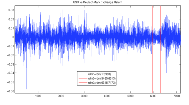
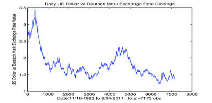
    The USA Dollar Exchange rate in Deusch-Mark, from 11/10/19831110198311/10/1983 to 08/04/20110804201108/04/2011 (717471747174 obs.).

  2. 2.

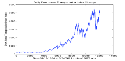
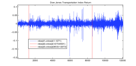
    The USA Dow Jones Transportation Index, from 31/12/19643112196431/12/1964 to 08/04/20110804201108/04/2011 (120721207212072 obs.).

  3. 3.

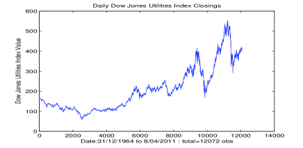
    The USA Dow Jones Utilities Index, from 31/12/19643112196431/12/1964 to 08/04/20110804201108/04/2011 (120721207212072 obs.).

  4. 4.

    The USA Nasdaq Industrials Index, from 05/02/19710502197105/02/1971 to 08/04/20110804201108/04/2011 (104811048110481 obs.).

  5. 5.

    The Japan Nikkei225A Index, from 03/04/19500304195003/04/1950 to 8/04/201180420118/04/2011 (159201592015920 obs.).

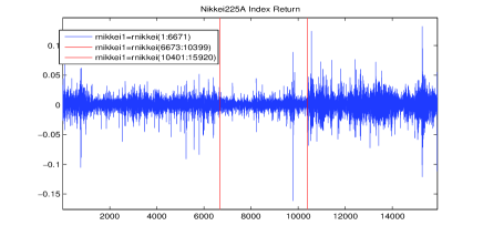
We considered the log-return of this data and tried to test their stationarity properties. Since stationarity or nonstationarity tests are not able to detect (offline) changes, we first used an algorithm developed by M. Lavielle for detecting changes (this free software can be downloaded from his homepage: http://www.math.u-psud.fr/similar-to\simlavielle/programmes¯¯absent\overline{\leavevmode\nobreak\ }lavielle.html). This algorithm provides the choice of detecting changes in mean, in variance, …, and we chose to detect parametric changes in the distribution. Note that the number of changes is also estimated since this algorithm is based on the minimization of a penalized contrast. We obtained for each time series an estimated number of changes equal to 222 which are the following:

  • Two breaks points for the US dollar-Deutsch Mark Exchange rate return are estimated, corresponding to the dates: 21/08/2006 and 24/12/2007. The Financial crisis of 2007-2011, followed by the late 2000s recession and the 2010 European sovereign debt crisis can cause such breaks.

  • Both the breaks points estimated for the US Dow Jones Transportation Index return, of the New-York Stock Market, correspond to the dates: 17/11/1969 and 15/09/1997. The first break change can be a consequence on transportation companies difficulties the American Viet-Nam war against communist block. The second change point can be viewed as a contagion by the spread of the Thai crisis in 1997 to other countries and mainly the US stock Market.

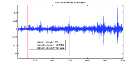
  • Both the breaks points estimated for the US Dow Jones Utilities Index return correspond to the dates: 02/06/1969 and 14/07/1998. The same arguments as above can justify the first break. The second at 1998 is probably a consequence of “the long very acute crisis in the bond markets,…, the dramatic fiscal crisis and Russian Flight to quality caused by it, may have been warning the largest known by the global financial system: we never went too close to a definitive breakdown of relations between the various financial instruments“(Wikipedia).

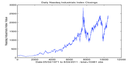
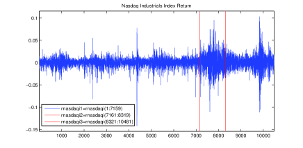
  • The two breaks points for the US Nasdaq Industrials Index return correspond to the dates: 17/07/1998 and 27/12/2002. The first break at 1998 is explained by the Russian flight to quality as above. The second break at 2002 corresponds to the Brazilian public debt crisis of 2002 toward foreign owners (mainly the U.S. and the IMF) which implicitly assigns a default of payment probability close to 100% with a direct impact on the financial markets indexes as the Nasdaq.

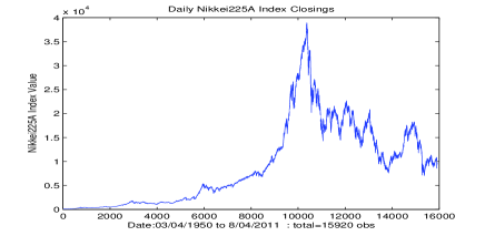
  • Both the breaks points estimated for the Japanese Nikkei225A Index return corresponds to the dates 29/10/1975 and 12/02/1990, perhaps as consequence of the strong dependency of Japan to the middle east Oil following 1974 or anticipating 1990 oil crisis. The credit crunch which is seen as a major factor in the U.S. recession of 1990-91 can play a role in the second break point.

Data and estimated instant breaks can be seen on Figure 1. Then, we applied the estimators and tests described in the previous subsection on trajectories obtained in each stages for the 555 economic time series. These applications were done on the log-returns, their absolute values, their squared values and their θ𝜃\theta-power laws with θ𝜃\theta maximized for each LRD estimators. The results of these numerical experiments can be seen in Tables 9-13.
 
Conclusions of numerical experiments: We exhibited again the well known result: the log-returns are stationary and short memory processes while absolute values or power θ𝜃\theta of log-returns are generally stationary but long memory processes (for this conclusion, we essentially consider the results of S~Nsubscript~𝑆𝑁\widetilde{S}_{N}, T~Nsubscript~𝑇𝑁\widetilde{T}_{N} and V/S tests since the other tests have been shown not to be relevant in the cases of long-memory processes). However the last and third estimated stage of each time series provides generally the largest estimated values of the memory parameter d𝑑d (for power law of log-returns) which are close to 0.50.50.5; hence, for Nasdaq time series, we accepted the nonstationarity assumption.
Refer to caption
Refer to caption
Refer to caption
Refer to caption
Refer to caption
Refer to caption
Refer to caption
Refer to caption
Refer to caption
Refer to caption
Figure 1: The financial data (DowJonesTransportations, DowJonesUtilities, NasdaqIndustrials, Nikkei225A and US Dollar vs Deutsch Mark): original data (left) and log-return with their both estimated breaks instants (right) occurred at the distribution Changes

r=(USD1 vs Deutsh-Mark Exchange Rate Return) Segments (Non)Stationarity Test LRD Kurtosis Skewness d^^𝑑\widehat{d} Breaks S~Nsubscript~𝑆𝑁\widetilde{S}_{N} T~Nsubscript~𝑇𝑁\widetilde{T}_{N} ADF PP KPSS LMC V/S𝑉𝑆V/S κ~~𝜅\widetilde{\kappa} s~~𝑠\widetilde{s} dIR~~superscript𝑑𝐼𝑅\widetilde{d^{IR}} dMS~~superscript𝑑𝑀𝑆\widetilde{d^{MS}} dADG^^superscript𝑑𝐴𝐷𝐺\widehat{d^{ADG}} dWAV~~superscript𝑑𝑊𝐴𝑉\widetilde{d^{WAV}} [1:5963]delimited-[]:15963[1:5963] S S S S S S SM 5.5 -0.2 -0.031 0.059 0.057 -0.007 [5965:6313]delimited-[]:59656313[5965:6313] S S S S S S SM 3.4 0.1 0.034 0.169 0.122 -0.015 [6315:7173]delimited-[]:63157173[6315:7173] S S S S S S SM 5.3 -0.4 0.098 0.140 0.043 0.019

|r|=abs(USD1 vs Deutsh-Mark Exchange Rate Return)𝑟𝑎𝑏𝑠USD1 vs Deutsh-Mark Exchange Rate Return|r|=abs(\mbox{USD1 vs Deutsh-Mark Exchange Rate Return}) Segments (Non)Stationarity Test LRD Kurtosis Skewness d^^𝑑\widehat{d} Breaks S~Nsubscript~𝑆𝑁\widetilde{S}_{N} T~Nsubscript~𝑇𝑁\widetilde{T}_{N} ADF PP KPSS LMC V/S𝑉𝑆V/S κ~~𝜅\widetilde{\kappa} s~~𝑠\widetilde{s} dIR~~superscript𝑑𝐼𝑅\widetilde{d^{IR}} dMS~~superscript𝑑𝑀𝑆\widetilde{d^{MS}} dADG^^superscript𝑑𝐴𝐷𝐺\widehat{d^{ADG}} dWAV~~superscript𝑑𝑊𝐴𝑉\widetilde{d^{WAV}} [1:5963]delimited-[]:15963[1:5963] S S S S NS NS LM 9.5 1.8 0.294 0.301 0.344 0.275 [5965:6313]delimited-[]:59656313[5965:6313] S S NS S NS NS LM 3.6 1.1 -0.121 0.153 0.414 -0.038 [6315:7173]delimited-[]:63157173[6315:7173] S S S S NS NS LM 9.2 1.8 0.168 0.417 0.389 0.410

r2=(USD1 vs Deutsh-Mark Exchange Rate Return)2superscript𝑟2superscriptUSD1 vs Deutsh-Mark Exchange Rate Return2r^{2}=(\mbox{USD1 vs Deutsh-Mark Exchange Rate Return})^{2} Segments (Non)Stationarity Test LRD Kurtosis Skewness d^^𝑑\widehat{d} Breaks S~Nsubscript~𝑆𝑁\widetilde{S}_{N} T~Nsubscript~𝑇𝑁\widetilde{T}_{N} ADF PP KPSS LMC V/S𝑉𝑆V/S κ~~𝜅\widetilde{\kappa} s~~𝑠\widetilde{s} dIR~~superscript𝑑𝐼𝑅\widetilde{d^{IR}} dMS~~superscript𝑑𝑀𝑆\widetilde{d^{MS}} dADG^^superscript𝑑𝐴𝐷𝐺\widehat{d^{ADG}} dWAV~~superscript𝑑𝑊𝐴𝑉\widetilde{d^{WAV}} [1:5963]delimited-[]:15963[1:5963] S S S S S S LM 289.5 10.7 0.081 0.258 0.298 0.078 [5965:6313]delimited-[]:59656313[5965:6313] S S S S NS S LM 8.7 2.3 -0.018 0.127 0.431 -0.096 [6315:7173]delimited-[]:63157173[6315:7173] S S S S NS S LM 81.3 7.1 0.035 0.411 0.336 0.428

|r|θ=(abs(USD1 vs Deutsh-Mark Exchange Rate Return))θsuperscript𝑟𝜃superscript𝑎𝑏𝑠USD1 vs Deutsh-Mark Exchange Rate Return𝜃|r|^{\theta}=(abs(\mbox{USD1 vs Deutsh-Mark Exchange Rate Return}))^{\theta} θ^i(j)=superscriptsubscript^𝜃𝑖𝑗absent\widehat{\theta}_{i}^{(j)}= (Non)Stationarity Test LRD Kurtosis Skewness d^^𝑑\widehat{d} ArgMaxθ(d^(|ri|θ))subscriptArgMax𝜃^𝑑superscriptsubscript𝑟𝑖𝜃\mbox{ArgMax}_{\theta}(\widehat{d}(|r_{i}|^{\theta})) S~Nsubscript~𝑆𝑁\widetilde{S}_{N} T~Nsubscript~𝑇𝑁\widetilde{T}_{N} ADF PP KPSS LMC V/S𝑉𝑆V/S κ~~𝜅\widetilde{\kappa} s~~𝑠\widetilde{s} dIR~~superscript𝑑𝐼𝑅\widetilde{d^{IR}} dMS~~superscript𝑑𝑀𝑆\widetilde{d^{MS}} dADG^^superscript𝑑𝐴𝐷𝐺\widehat{d^{ADG}} dWAV~~superscript𝑑𝑊𝐴𝑉\widetilde{d^{WAV}} θ^1IRsuperscriptsubscript^𝜃1𝐼𝑅\widehat{\theta}_{1}^{IR}=0.32 S S NS S NS NS SM 3.5 -0.5 0.321* 0.251 0.256 0.343 θ^1MSsuperscriptsubscript^𝜃1𝑀𝑆\widehat{\theta}_{1}^{MS}= 0.97 S S S S NS NS SM 8.7 1.1 0.293 0.301* 0.343 0.275 θ^1ADGsuperscriptsubscript^𝜃1𝐴𝐷𝐺\widehat{\theta}_{1}^{ADG}= 1.12 S S S S NS NS SM 13.7 2.3 0.302 0.300 0.345* 0.273 θ^1WAVsuperscriptsubscript^𝜃1𝑊𝐴𝑉\widehat{\theta}_{1}^{WAV}=0.77 S S S S NS NS SM 5.1 1.1 0.273 0.298 0.335 0.379* θ^2IRsuperscriptsubscript^𝜃2𝐼𝑅\widehat{\theta}_{2}^{IR}=0.05 S S NS NS S NS LM 27.9 -5.0 0.246* 0.078 -0.005 0.103 θ^2MSsuperscriptsubscript^𝜃2𝑀𝑆\widehat{\theta}_{2}^{MS}= 1.31 S S S S NS NS LM 4.9 1.5 -0.103 0.166* 0.446 -0.072 θ^2ADGsuperscriptsubscript^𝜃2𝐴𝐷𝐺\widehat{\theta}_{2}^{ADG}=1.50 S S S S NS S LM 5.8 1.8 -0.092 0.162 0.450* -0.082 θ^2WAVsuperscriptsubscript^𝜃2𝑊𝐴𝑉\widehat{\theta}_{2}^{WAV}=0.03 S S NS NS S NS LM 30.9 -5.4 0.239 0.113 -0.030 0.211* θ^3IRsuperscriptsubscript^𝜃3𝐼𝑅\widehat{\theta}_{3}^{IR}=0.63 S S NS NS NS NS LM 3.8 0.7 0.244* 0.354 0.333 0.097 θ^3MSsuperscriptsubscript^𝜃3𝑀𝑆\widehat{\theta}_{3}^{MS}= 1.44 S S S S NS NS LM 27.1 3.7 0.159 0.436* 0.387 0.441 θ^3ADGsuperscriptsubscript^𝜃3𝐴𝐷𝐺\widehat{\theta}_{3}^{ADG}= 1.19 S S S S NS NS LM 14.9 2.6 0.168 0.430 0.394* 0.430 θ^3WAVsuperscriptsubscript^𝜃3𝑊𝐴𝑉\widehat{\theta}_{3}^{WAV}= 2.90 S S S S NS S LM 223.4 13.3 0.053 0.291 0.233 0.475*

Table 9: Results of stationarity, nonstationarity and V/S tests and the 444 long memory parameter estimators applied to several functionals f𝑓f of USD1 vs Deutsh-Mark Exchange Rate Return: from the top to bottom, f(x)=x𝑓𝑥𝑥f(x)=x, f(x)=|x|𝑓𝑥𝑥f(x)=|x|, f(x)=x2𝑓𝑥superscript𝑥2f(x)=x^{2} and f(x)=|x|θ𝑓𝑥superscript𝑥𝜃f(x)=|x|^{\theta} with θ𝜃\theta maximizing the 444 different long memory parameter estimators (”S𝑆S“ for ”stationarity“ decision and ”NS𝑁𝑆NS“ for ”nonstationarity“ decision). Statistics are applied to the 333 estimated stages of each trajectory (obtained from a change detection algorithm).

r=Dow Jones Transportation Index Return Segments (Non)Stationarity Test LRD Kurtosis Skewness d^^𝑑\widehat{d} Breaks S~Nsubscript~𝑆𝑁\widetilde{S}_{N} T~Nsubscript~𝑇𝑁\widetilde{T}_{N} ADF PP KPSS LMC V/S𝑉𝑆V/S κ~~𝜅\widetilde{\kappa} s~~𝑠\widetilde{s} dIR~~superscript𝑑𝐼𝑅\widetilde{d^{IR}} dMS~~superscript𝑑𝑀𝑆\widetilde{d^{MS}} dADG^^superscript𝑑𝐴𝐷𝐺\widehat{d^{ADG}} dWAV~~superscript𝑑𝑊𝐴𝑉\widetilde{d^{WAV}} [1:1271]delimited-[]:11271[1:1271] S S S S S NS SM 4.6 0.0 0.218 0.174 0.098 0.198 [1273:8531]delimited-[]:12738531[1273:8531] S S S S S S SM 21.7 -0.8 0.053 0.002 0.008 -0.404 [8533:12071]delimited-[]:853312071[8533:12071] S S S S S S SM 8.3 -0.3 0.002 -0.015 -0.034 -0.038

|r|=abs(Dow Jones Transportation Index Return)𝑟𝑎𝑏𝑠Dow Jones Transportation Index Return|r|=abs(\mbox{Dow Jones Transportation Index Return}) Segments (Non)Stationarity Test LRD Kurtosis Skewness d^^𝑑\widehat{d} Breaks S~Nsubscript~𝑆𝑁\widetilde{S}_{N} T~Nsubscript~𝑇𝑁\widetilde{T}_{N} ADF PP KPSS LMC V/S𝑉𝑆V/S κ~~𝜅\widetilde{\kappa} s~~𝑠\widetilde{s} dIR~~superscript𝑑𝐼𝑅\widetilde{d^{IR}} dMS~~superscript𝑑𝑀𝑆\widetilde{d^{MS}} dADG^^superscript𝑑𝐴𝐷𝐺\widehat{d^{ADG}} dWAV~~superscript𝑑𝑊𝐴𝑉\widetilde{d^{WAV}} [1:1272]delimited-[]:11272[1:1272] S S S S NS NS LM 6.1 1.5 0.154 0.320 0.270 0.166 [1273:8532]delimited-[]:12738532[1273:8532] S S S S NS NS LM 57.3 4.4 0.322 0.260 0.240 0.168 [8533:12071]delimited-[]:853312071[8533:12071] S S S S NS NS LM 16.3 2.5 0.405 0.476 0.496 0.374

r2=(Dow Jones Transportation Index Return)2superscript𝑟2superscriptDow Jones Transportation Index Return2r^{2}=(\mbox{Dow Jones Transportation Index Return})^{2} Segments (Non)Stationarity Test LRD Kurtosis Skewness d^^𝑑\widehat{d} Breaks S~Nsubscript~𝑆𝑁\widetilde{S}_{N} T~Nsubscript~𝑇𝑁\widetilde{T}_{N} ADF PP KPSS LMC V/S𝑉𝑆V/S κ~~𝜅\widetilde{\kappa} s~~𝑠\widetilde{s} dIR~~superscript𝑑𝐼𝑅\widetilde{d^{IR}} dMS~~superscript𝑑𝑀𝑆\widetilde{d^{MS}} dADG^^superscript𝑑𝐴𝐷𝐺\widehat{d^{ADG}} dWAV~~superscript𝑑𝑊𝐴𝑉\widetilde{d^{WAV}} [1:1272]delimited-[]:11272[1:1272] S S S S NS S LM 32.3 4.4 0.158 0.284 0.231 0.231 [1273:8532]delimited-[]:12738532[1273:8532] S S S S S NS LM 2301.5 39.9 0.334 0.122 0.093 0.118 [8533:12071]delimited-[]:853312071[8533:12071] S NS S S NS NS LM 459.0 15.5 0.416 0.452 0.434 0.356

|r|θ=(abs(Dow Jones Transportation Index Return))θsuperscript𝑟𝜃superscript𝑎𝑏𝑠Dow Jones Transportation Index Return𝜃|r|^{\theta}=(abs(\mbox{Dow Jones Transportation Index Return}))^{\theta} θ^i(j)=superscriptsubscript^𝜃𝑖𝑗absent\widehat{\theta}_{i}^{(j)}= (Non)Stationarity Test LRD Kurtosis Skewness d^^𝑑\widehat{d} ArgMaxθ(d^(|ri|θ)\mbox{ArgMax}_{\theta}(\widehat{d}(|r_{i}|^{\theta}) S~Nsubscript~𝑆𝑁\widetilde{S}_{N} T~Nsubscript~𝑇𝑁\widetilde{T}_{N} ADF PP KPSS LMC V/S𝑉𝑆V/S κ~~𝜅\widetilde{\kappa} s~~𝑠\widetilde{s} dIR~~superscript𝑑𝐼𝑅\widetilde{d^{IR}} dMS~~superscript𝑑𝑀𝑆\widetilde{d^{MS}} dADG^^superscript𝑑𝐴𝐷𝐺\widehat{d^{ADG}} dWAV~~superscript𝑑𝑊𝐴𝑉\widetilde{d^{WAV}} θ^1IRsuperscriptsubscript^𝜃1𝐼𝑅\widehat{\theta}_{1}^{IR}= 1.83 S S S S NS S LM 25.0 3.8 0.252* 0.291 0.237 0.202 θ^1MSsuperscriptsubscript^𝜃1𝑀𝑆\widehat{\theta}_{1}^{MS}= 0.45 S S NS S NS NS LM 2.7 0.4 0.118 0.331* 0.290 0.047 θ^1ADGsuperscriptsubscript^𝜃1𝐴𝐷𝐺\widehat{\theta}_{1}^{ADG}= 0.36 S S NS S NS NS LM 2.9 -0.4 0.118 0.329 0.291* 0.237 θ^1WAVsuperscriptsubscript^𝜃1𝑊𝐴𝑉\widehat{\theta}_{1}^{WAV}= 0.03 S S NS S NS NS LM 12.8 -3.4 0.149 0.257 0.260 0.327* θ^2IRsuperscriptsubscript^𝜃2𝐼𝑅\widehat{\theta}_{2}^{IR}= 2.06 S S S S S NS LM 2551.6 42.6 0.355* 0.113 0.086 0.110 θ^2MSsuperscriptsubscript^𝜃2𝑀𝑆\widehat{\theta}_{2}^{MS}= 0.68 S S S S NS NS LM 10.6 1.6 0.308 0.276* 0.261 0.135 θ^2ADGsuperscriptsubscript^𝜃2𝐴𝐷𝐺\widehat{\theta}_{2}^{ADG}= 0.65 S S S S NS NS LM 9.2 1.4 0.303 0.276 0.261* 0.129 θ^2WAVsuperscriptsubscript^𝜃2𝑊𝐴𝑉\widehat{\theta}_{2}^{WAV}= 1.29 S S S S NS NS LM 246.8 10.1 0.330 0.227 0.200 0.504* θ^3IRsuperscriptsubscript^𝜃3𝐼𝑅\widehat{\theta}_{3}^{IR}= 0.66 S NS S S NS NS LM 5.4 1.1 0.444* 0.435 0.461 0.374 θ^3MSsuperscriptsubscript^𝜃3𝑀𝑆\widehat{\theta}_{3}^{MS}= 1.38 S S S S NS NS LM 64.8 5.2 0.402 0.492* 0.499 0.391 θ^3ADGsuperscriptsubscript^𝜃3𝐴𝐷𝐺\widehat{\theta}_{3}^{ADG}= 1.22 S S S S NS NS LM 36.2 3.8 0.400 0.489 0.502* 0.387 θ^3WAVsuperscriptsubscript^𝜃3𝑊𝐴𝑉\widehat{\theta}_{3}^{WAV}= 2.75 S S S S NS NS LM 1698.7 35.8 0.407 0.315 0.287 0.466*

Table 10: Results of stationarity, nonstationarity and V/S tests and the 444 long memory parameter estimators applied to several functionals f𝑓f of DowJones Transportation Index Return: from the top to bottom, f(x)=x𝑓𝑥𝑥f(x)=x, f(x)=|x|𝑓𝑥𝑥f(x)=|x|, f(x)=x2𝑓𝑥superscript𝑥2f(x)=x^{2} and f(x)=|x|θ𝑓𝑥superscript𝑥𝜃f(x)=|x|^{\theta} with θ𝜃\theta maximizing the 444 different long memory parameter estimators (”S𝑆S“ for ”stationarity“ decision and ”NS𝑁𝑆NS“ for ”nonstationarity“ decision). Statistics are applied to the 333 estimated stages of each trajectory (obtained from a change detection algorithm).

r=Dow Jones Utilities Index Return Segments (Non)Stationarity Test LRD Kurtosis Skewness d^^𝑑\widehat{d} Breaks S~Nsubscript~𝑆𝑁\widetilde{S}_{N} T~Nsubscript~𝑇𝑁\widetilde{T}_{N} ADF PP KPSS LMC V/S𝑉𝑆V/S κ~~𝜅\widetilde{\kappa} s~~𝑠\widetilde{s} dIR~~superscript𝑑𝐼𝑅\widetilde{d^{IR}} dMS~~superscript𝑑𝑀𝑆\widetilde{d^{MS}} dADG^^superscript𝑑𝐴𝐷𝐺\widehat{d^{ADG}} dWAV~~superscript𝑑𝑊𝐴𝑉\widetilde{d^{WAV}} [1:1152]delimited-[]:11152[1:1152] S S S S S S SM 7.3 0.6 0.191 0.037 -0.132 0.222 [1153:8748]delimited-[]:11538748[1153:8748] S S S S S S SM 43.2 -1.3 0.094 0.025 0.001 0.043 [8749:12071]delimited-[]:874912071[8749:12071] S S S S S S SM 13.0 0.0 0.026 0.024 0.001 -0.032

|r|=abs(Dow Jones Utilities Index Return)𝑟𝑎𝑏𝑠Dow Jones Utilities Index Return|r|=abs(\mbox{Dow Jones Utilities Index Return}) Segments (Non)Stationarity Test LRD Kurtosis Skewness d^^𝑑\widehat{d} Breaks S~Nsubscript~𝑆𝑁\widetilde{S}_{N} T~Nsubscript~𝑇𝑁\widetilde{T}_{N} ADF PP KPSS LMC V/S𝑉𝑆V/S κ~~𝜅\widetilde{\kappa} s~~𝑠\widetilde{s} dIR~~superscript𝑑𝐼𝑅\widetilde{d^{IR}} dMS~~superscript𝑑𝑀𝑆\widetilde{d^{MS}} dADG^^superscript𝑑𝐴𝐷𝐺\widehat{d^{ADG}} dWAV~~superscript𝑑𝑊𝐴𝑉\widetilde{d^{WAV}} [1:1152]delimited-[]:11152[1:1152] S S S S NS NS LM 11.9 2.4 0.283 0.287 0.316 0.225 [1153:8748]delimited-[]:11538748[1153:8748] S S S S NS NS LM 127.4 5.9 0.134 0.301 0.304 0.184 [8749:12071]delimited-[]:874912071[8749:12071] S S S S NS NS LM 25.5 3.4 0.417 0.559 0.484 0.595

r2=(Dow Jones Utilities Index Return)2superscript𝑟2superscriptDow Jones Utilities Index Return2r^{2}=(\mbox{Dow Jones Utilities Index Return})^{2} Segments (Non)Stationarity Test LRD Kurtosis Skewness d^^𝑑\widehat{d} Breaks S~Nsubscript~𝑆𝑁\widetilde{S}_{N} T~Nsubscript~𝑇𝑁\widetilde{T}_{N} ADF PP KPSS LMC V/S𝑉𝑆V/S κ~~𝜅\widetilde{\kappa} s~~𝑠\widetilde{s} dIR~~superscript𝑑𝐼𝑅\widetilde{d^{IR}} dMS~~superscript𝑑𝑀𝑆\widetilde{d^{MS}} dADG^^superscript𝑑𝐴𝐷𝐺\widehat{d^{ADG}} dWAV~~superscript𝑑𝑊𝐴𝑉\widetilde{d^{WAV}} [1:1152]delimited-[]:11152[1:1152] S S S S NS S LM 63.1 6.7 0.250 0.253 0.212 0.270 [1153:8748]delimited-[]:11538748[1153:8748] S S S S NS NS LM 5322.4 67.8 0.130 0.100 0.100 0.100 [8749:12071]delimited-[]:874912071[8749:12071] S NS S S NS NS LM 289.6 14.0 0.510 0.468 0.423 0.513

|r|θ=(abs(Dow Jones Utilities Index Return))θsuperscript𝑟𝜃superscript𝑎𝑏𝑠Dow Jones Utilities Index Return𝜃|r|^{\theta}=(abs(\mbox{Dow Jones Utilities Index Return}))^{\theta} θ^i(j)=superscriptsubscript^𝜃𝑖𝑗absent\widehat{\theta}_{i}^{(j)}= (Non)Stationarity Test LRD Kurtosis Skewness d^^𝑑\widehat{d} ArgMaxθ(d^(|ri|θ))subscriptArgMax𝜃^𝑑superscriptsubscript𝑟𝑖𝜃\mbox{ArgMax}_{\theta}(\widehat{d}(|r_{i}|^{\theta})) S~Nsubscript~𝑆𝑁\widetilde{S}_{N} T~Nsubscript~𝑇𝑁\widetilde{T}_{N} ADF PP KPSS LMC V/S𝑉𝑆V/S κ~~𝜅\widetilde{\kappa} s~~𝑠\widetilde{s} dIR~~superscript𝑑𝐼𝑅\widetilde{d^{IR}} dMS~~superscript𝑑𝑀𝑆\widetilde{d^{MS}} dADG^^superscript𝑑𝐴𝐷𝐺\widehat{d^{ADG}} dWAV~~superscript𝑑𝑊𝐴𝑉\widetilde{d^{WAV}} θ^1IR=0.39superscriptsubscript^𝜃1𝐼𝑅0.39\widehat{\theta}_{1}^{IR}=0.39 S S NS S NS NS LM 3.3 -0.1 0.354* 0.262 0.327 0.145 θ^1MS=1.09superscriptsubscript^𝜃1𝑀𝑆1.09\widehat{\theta}_{1}^{MS}=1.09 S S S S NS NS LM 14.6 8.4 0.215 0.288* 0.308 0.234 θ^1ADG=0.60superscriptsubscript^𝜃1𝐴𝐷𝐺0.60\widehat{\theta}_{1}^{ADG}=0.60 S S NS S NS NS LM 4.5 0.8 0.311 0.276 0.336* 0.396 θ^1WAV=0.63superscriptsubscript^𝜃1𝑊𝐴𝑉0.63\widehat{\theta}_{1}^{WAV}=0.63 S S S S NS NS LM 4.8 1.0 0.310 0.278 0.336 0.398* θ^2IR=3.00superscriptsubscript^𝜃2𝐼𝑅3.00\widehat{\theta}_{2}^{IR}=3.00 S S S S S S LM 7320.6 84.9 0.165* 0.015 0.017 0.040 θ^2MS=0.61superscriptsubscript^𝜃2𝑀𝑆0.61\widehat{\theta}_{2}^{MS}=0.61 S S S S NS NS LM 9.1 1.2 0.113 0.330* 0.327 0.113 θ^2ADG=0.67superscriptsubscript^𝜃2𝐴𝐷𝐺0.67\widehat{\theta}_{2}^{ADG}=0.67 S S S S NS NS LM 13.0 1.6 0.117 0.330 0.327* 0.113 θ^2WAV=1.84superscriptsubscript^𝜃2𝑊𝐴𝑉1.84\widehat{\theta}_{2}^{WAV}=1.84 S S S S NS NS LM 4386.6 59.1 0.125 0.130 0.129 0.377* θ^3IR=2.69superscriptsubscript^𝜃3𝐼𝑅2.69\widehat{\theta}_{3}^{IR}=2.69 S NS S S NS NS LM 683.1 22.5 0.527* 0.394 0.344 0.426 θ^3MS=0.95superscriptsubscript^𝜃3𝑀𝑆0.95\widehat{\theta}_{3}^{MS}=0.95 S S S S NS NS LM 21.6 3.1 0.415 0.560* 0.483 0.544 θ^3ADG=1.10superscriptsubscript^𝜃3𝐴𝐷𝐺1.10\widehat{\theta}_{3}^{ADG}=1.10 S S S S NS NS LM 35.2 4.2 0.421 0.557 0.485* 0.364 θ^3WAV=1.03superscriptsubscript^𝜃3𝑊𝐴𝑉1.03\widehat{\theta}_{3}^{WAV}=1.03 S S S S NS NS LM 28.2 3.7 0.419 0.559 0.484 0.723*

Table 11: Results of stationarity, nonstationarity and V/S tests and the 444 long memory parameter estimators applied to several functionals f𝑓f of Dow Jones Utilities Index Return: from the top to bottom, f(x)=x𝑓𝑥𝑥f(x)=x, f(x)=|x|𝑓𝑥𝑥f(x)=|x|, f(x)=x2𝑓𝑥superscript𝑥2f(x)=x^{2} and f(x)=|x|θ𝑓𝑥superscript𝑥𝜃f(x)=|x|^{\theta} with θ𝜃\theta maximizing the 444 different long memory parameter estimators (”S𝑆S“ for ”stationarity“ decision and ”NS𝑁𝑆NS“ for ”nonstationarity“ decision). Statistics are applied to the 333 estimated stages of each trajectory (obtained from a change detection algorithm).

r=Nasdaq Industrials Index Return Segments (Non)Stationarity Test LRD Kurtosis Skewness d^^𝑑\widehat{d} Breaks S~Nsubscript~𝑆𝑁\widetilde{S}_{N} T~Nsubscript~𝑇𝑁\widetilde{T}_{N} ADF PP KPSS LMC V/S𝑉𝑆V/S κ~~𝜅\widetilde{\kappa} s~~𝑠\widetilde{s} dIR~~superscript𝑑𝐼𝑅\widetilde{d^{IR}} dMS~~superscript𝑑𝑀𝑆\widetilde{d^{MS}} dADG^^superscript𝑑𝐴𝐷𝐺\widehat{d^{ADG}} dWAV~~superscript𝑑𝑊𝐴𝑉\widetilde{d^{WAV}} [1:7160]delimited-[]:17160[1:7160] S S S S S S SM 20.7 -1.5 0.141 0.073 0.092 -0.202 [7161:8320]delimited-[]:71618320[7161:8320] S S S S S S SM 4.6 0.0 0.012 0.070 0.116 0.014 [8321:10480]delimited-[]:832110480[8321:10480] S S S S NS S SM 10.4 -0.3 0.045 0.078 0.082 -0.045

|r|=abs(Nasdaq Industrials Index Return)𝑟𝑎𝑏𝑠Nasdaq Industrials Index Return|r|=abs(\mbox{Nasdaq Industrials Index Return}) Segments (Non)Stationarity Test LRD Kurtosis Skewness d^^𝑑\widehat{d} Breaks S~Nsubscript~𝑆𝑁\widetilde{S}_{N} T~Nsubscript~𝑇𝑁\widetilde{T}_{N} ADF PP KPSS LMC V/S𝑉𝑆V/S κ~~𝜅\widetilde{\kappa} s~~𝑠\widetilde{s} dIR~~superscript𝑑𝐼𝑅\widetilde{d^{IR}} dMS~~superscript𝑑𝑀𝑆\widetilde{d^{MS}} dADG^^superscript𝑑𝐴𝐷𝐺\widehat{d^{ADG}} dWAV~~superscript𝑑𝑊𝐴𝑉\widetilde{d^{WAV}} [1:7160]delimited-[]:17160[1:7160] S S S S S NS SM 52.4 4.4 0.361 0.309 0.287 0.274 [7161:8320]delimited-[]:71618320[7161:8320] S S S S NS NS LM 7.4 1.6 0.284 0.532 0.504 0.385 [8321:10480]delimited-[]:832110480[8321:10480] S NS S NS NS NS LM 18.3 3.0 0.516 0.761 0.606 0.668

r2=(Nasdaq Industrials Index Return)2superscript𝑟2superscriptNasdaq Industrials Index Return2r^{2}=(\mbox{Nasdaq Industrials Index Return})^{2} Segments (Non)Stationarity Test LRD Kurtosis Skewness d^^𝑑\widehat{d} Breaks S~Nsubscript~𝑆𝑁\widetilde{S}_{N} T~Nsubscript~𝑇𝑁\widetilde{T}_{N} ADF PP KPSS LMC V/S𝑉𝑆V/S κ~~𝜅\widetilde{\kappa} s~~𝑠\widetilde{s} dIR~~superscript𝑑𝐼𝑅\widetilde{d^{IR}} dMS~~superscript𝑑𝑀𝑆\widetilde{d^{MS}} dADG^^superscript𝑑𝐴𝐷𝐺\widehat{d^{ADG}} dWAV~~superscript𝑑𝑊𝐴𝑉\widetilde{d^{WAV}} [1:7160]delimited-[]:17160[1:7160] S S S S S NS SM 1356.8 31.4 0.381 0.146 0.114 0.100 [7161:8320]delimited-[]:71618320[7161:8320] S S S S NS NS LM 49.0 5.4 0.304 0.466 0.378 0.432 [8321:10480]delimited-[]:832110480[8321:10480] S NS S S NS NS LM 140.0 10.0 0.498 0.786 0.544 0.708

|r|θ=(abs(Nasdaq Industrials Index Return))θsuperscript𝑟𝜃superscript𝑎𝑏𝑠Nasdaq Industrials Index Return𝜃|r|^{\theta}=(abs(\mbox{Nasdaq Industrials Index Return}))^{\theta} θ^i(j)=superscriptsubscript^𝜃𝑖𝑗absent\widehat{\theta}_{i}^{(j)}= (Non)Stationarity Test LRD Kurtosis Skewness d^^𝑑\widehat{d} ArgMaxθ(d^(|ri|θ))subscriptArgMax𝜃^𝑑superscriptsubscript𝑟𝑖𝜃\mbox{ArgMax}_{\theta}(\widehat{d}(|r_{i}|^{\theta})) S~Nsubscript~𝑆𝑁\widetilde{S}_{N} T~Nsubscript~𝑇𝑁\widetilde{T}_{N} ADF PP KPSS LMC V/S𝑉𝑆V/S κ~~𝜅\widetilde{\kappa} s~~𝑠\widetilde{s} dIR~~superscript𝑑𝐼𝑅\widetilde{d^{IR}} dMS~~superscript𝑑𝑀𝑆\widetilde{d^{MS}} dADG^^superscript𝑑𝐴𝐷𝐺\widehat{d^{ADG}} dWAV~~superscript𝑑𝑊𝐴𝑉\widetilde{d^{WAV}} θ^1IR=1.04superscriptsubscript^𝜃1𝐼𝑅1.04\widehat{\theta}_{1}^{IR}=1.04 S S S S S NS LM 63.7 4.9 0.396* 0.304 0.281 0.325 θ^1MS=0.67superscriptsubscript^𝜃1𝑀𝑆0.67\widehat{\theta}_{1}^{MS}=0.67 S S S S NS NS LM 10.2 0.7 0.188 0.329* 0.325 0.293 θ^1ADG=0.56superscriptsubscript^𝜃1𝐴𝐷𝐺0.56\widehat{\theta}_{1}^{ADG}=0.56 S S S S NS NS LM 6.3 0.9 0.178 0.326 0.328* 0.275 θ^1WAV=0.83superscriptsubscript^𝜃1𝑊𝐴𝑉0.83\widehat{\theta}_{1}^{WAV}=0.83 S S S S NS NS LM 22.4 2.6 0.199 0.324 0.311 0.587* θ^2IR=2.83superscriptsubscript^𝜃2𝐼𝑅2.83\widehat{\theta}_{2}^{IR}=2.83 S S S S NS S LM 142.0 9.8 0.317* 0.374 0.276 0.263 θ^2MS=1.03superscriptsubscript^𝜃2𝑀𝑆1.03\widehat{\theta}_{2}^{MS}=1.03 S S S S NS NS LM 7.9 1.7 0.284 0.532* 0.501 0.388 θ^2ADG=0.73superscriptsubscript^𝜃2𝐴𝐷𝐺0.73\widehat{\theta}_{2}^{ADG}=0.73 S S NS S NS NS LM 4.2 0.9 0.300 0.517 0.517* 0.340 θ^2WAV=1.87superscriptsubscript^𝜃2𝑊𝐴𝑉1.87\widehat{\theta}_{2}^{WAV}=1.87 S S S S NS NS LM 39.8 4.8 0.299 0.479 0.395 0.432* θ^3IR=2.60superscriptsubscript^𝜃3𝐼𝑅2.60\widehat{\theta}_{3}^{IR}=2.60 S NS S S NS S LM 256.9 14.3 0.548* 0.272 0.479 0.669 θ^3MS=1.70superscriptsubscript^𝜃3𝑀𝑆1.70\widehat{\theta}_{3}^{MS}=1.70 S NS S S NS NS LM 89.1 7.7 0.504 0.801* 0.575 0.739 θ^3ADG=1.13superscriptsubscript^𝜃3𝐴𝐷𝐺1.13\widehat{\theta}_{3}^{ADG}=1.13 S NS S S NS NS LM 26.0 3.7 0.526 0.772 0.608* 0.671 θ^3WAV=1.26superscriptsubscript^𝜃3𝑊𝐴𝑉1.26\widehat{\theta}_{3}^{WAV}=1.26 S NS S S NS NS LM 36.0 4.5 0.532 0.782 0.606 0.760*

Table 12: Results of stationarity, nonstationarity and V/S tests and the 444 long memory parameter estimators applied to several functionals f𝑓f of Nasdaq Industrials Index Return: from the top to bottom, f(x)=x𝑓𝑥𝑥f(x)=x, f(x)=|x|𝑓𝑥𝑥f(x)=|x|, f(x)=x2𝑓𝑥superscript𝑥2f(x)=x^{2} and f(x)=|x|θ𝑓𝑥superscript𝑥𝜃f(x)=|x|^{\theta} with θ𝜃\theta maximizing the 444 different long memory parameter estimators (”S𝑆S“ for ”stationarity“ decision and ”NS𝑁𝑆NS“ for ”nonstationarity“ decision). Statistics are applied to the 333 estimated stages of each trajectory (obtained from a change detection algorithm).

r=Nikkei 225A Index Return Segments (Non)Stationarity Test LRD Kurtosis Skewness d^^𝑑\widehat{d} Breaks S~Nsubscript~𝑆𝑁\widetilde{S}_{N} T~Nsubscript~𝑇𝑁\widetilde{T}_{N} ADF PP KPSS LMC V/S𝑉𝑆V/S κ~~𝜅\widetilde{\kappa} s~~𝑠\widetilde{s} dIR~~superscript𝑑𝐼𝑅\widetilde{d^{IR}} dMS~~superscript𝑑𝑀𝑆\widetilde{d^{MS}} dADG^^superscript𝑑𝐴𝐷𝐺\widehat{d^{ADG}} dWAV~~superscript𝑑𝑊𝐴𝑉\widetilde{d^{WAV}} [1:6672]delimited-[]:16672[1:6672] S S S S S S SM 12.6 -0.6 0.083 0.067 0.084 0.022 [6673:10400]delimited-[]:667310400[6673:10400] S S S S S S SM 63.7 -2.3 -0.021 -0.016 -0.013 -0.039 [10401:15919]delimited-[]:1040115919[10401:15919] S S S S S S SM 9.0 -0.1 0.033 0.047 -0.005 -0.015

|r|=abs(Nikkei 225A Index Return)𝑟𝑎𝑏𝑠Nikkei 225A Index Return|r|=abs(\mbox{Nikkei 225A Index Return}) Segments (Non)Stationarity Test LRD Kurtosis Skewness d^^𝑑\widehat{d} Breaks S~Nsubscript~𝑆𝑁\widetilde{S}_{N} T~Nsubscript~𝑇𝑁\widetilde{T}_{N} ADF PP KPSS LMC V/S𝑉𝑆V/S κ~~𝜅\widetilde{\kappa} s~~𝑠\widetilde{s} dIR~~superscript𝑑𝐼𝑅\widetilde{d^{IR}} dMS~~superscript𝑑𝑀𝑆\widetilde{d^{MS}} dADG^^superscript𝑑𝐴𝐷𝐺\widehat{d^{ADG}} dWAV~~superscript𝑑𝑊𝐴𝑉\widetilde{d^{WAV}} [1:6672]delimited-[]:16672[1:6672] S S S S NS NS LM 26.1 3.3 0.302 0.343 0.313 0.218 [6673:10400]delimited-[]:667310400[6673:10400] S S S S NS NS LM 150.9 7.5 0.196 0.346 0.304 0.321 [10401:15919]delimited-[]:1040115919[10401:15919] S S S S NS NS LM 17.0 2.6 0.413 0.415 0.431 0.335

r2=(Nikkei 225A Index Return)2superscript𝑟2superscriptNikkei 225A Index Return2r^{2}=(\mbox{Nikkei 225A Index Return})^{2} Segments (Non)Stationarity Test LRD Kurtosis Skewness d^^𝑑\widehat{d} Breaks S~Nsubscript~𝑆𝑁\widetilde{S}_{N} T~Nsubscript~𝑇𝑁\widetilde{T}_{N} ADF PP KPSS LMC V/S𝑉𝑆V/S κ~~𝜅\widetilde{\kappa} s~~𝑠\widetilde{s} dIR~~superscript𝑑𝐼𝑅\widetilde{d^{IR}} dMS~~superscript𝑑𝑀𝑆\widetilde{d^{MS}} dADG^^superscript𝑑𝐴𝐷𝐺\widehat{d^{ADG}} dWAV~~superscript𝑑𝑊𝐴𝑉\widetilde{d^{WAV}} [1:6672]delimited-[]:16672[1:6672] S S S S NS NS LM 427.8 16.9 0.275 0.241 0.267 0.080 [6673:10400]delimited-[]:667310400[6673:10400] S S S S S NS LM 2610.8 48.0 0.230 0.146 0.154 0.117 [10401:15919]delimited-[]:1040115919[10401:15919] S S S S NS NS LM 235.5 12.3 0.381 0.396 0.363 0.377

|r|θ=(abs(Nikkei 225A Index Return))θsuperscript𝑟𝜃superscript𝑎𝑏𝑠Nikkei 225A Index Return𝜃|r|^{\theta}=(abs(\mbox{Nikkei 225A Index Return}))^{\theta} θ^i(j)=superscriptsubscript^𝜃𝑖𝑗absent\widehat{\theta}_{i}^{(j)}= (Non)Stationarity Test LRD Kurtosis Skewness d^^𝑑\widehat{d} ArgMaxθ(d^(|ri|θ))subscriptArgMax𝜃^𝑑superscriptsubscript𝑟𝑖𝜃\mbox{ArgMax}_{\theta}(\widehat{d}(|r_{i}|^{\theta})) S~Nsubscript~𝑆𝑁\widetilde{S}_{N} T~Nsubscript~𝑇𝑁\widetilde{T}_{N} ADF PP KPSS LMC V/S𝑉𝑆V/S κ~~𝜅\widetilde{\kappa} s~~𝑠\widetilde{s} dIR~~superscript𝑑𝐼𝑅\widetilde{d^{IR}} dMS~~superscript𝑑𝑀𝑆\widetilde{d^{MS}} dADG^^superscript𝑑𝐴𝐷𝐺\widehat{d^{ADG}} dWAV~~superscript𝑑𝑊𝐴𝑉\widetilde{d^{WAV}} θ^1IR=1.53superscriptsubscript^𝜃1𝐼𝑅1.53\widehat{\theta}_{1}^{IR}=1.53 S S S S NS NS LM 149.8 9.0 0.323* 0.296 0.296 0.201 θ^1MS=0.86superscriptsubscript^𝜃1𝑀𝑆0.86\widehat{\theta}_{1}^{MS}=0.86 S S S S NS NS LM 15.4 4.4 0.286 0.345* 0.311 0.213 θ^1ADG=1.01superscriptsubscript^𝜃1𝐴𝐷𝐺1.01\widehat{\theta}_{1}^{ADG}=1.01 S S S S NS NS LM 27.1 3.4 0.303 0.342 0.313* 0.218 θ^1WAV=1.30superscriptsubscript^𝜃1𝑊𝐴𝑉1.30\widehat{\theta}_{1}^{WAV}=1.30 S S S S NS NS LM 74.8 6.1 0.273 0.322 0.307 0.622* θ^2IR=3.00superscriptsubscript^𝜃2𝐼𝑅3.00\widehat{\theta}_{2}^{IR}=3.00 S S S S S S LM 3487.4 58.3 0.252* 0.037 0.042 0.045 θ^2MS=0.84superscriptsubscript^𝜃2𝑀𝑆0.84\widehat{\theta}_{2}^{MS}=0.84 S S S S NS NS SM 55.5 4.1 0.180 0.353* 0.304 0.154 θ^2ADG=0.91superscriptsubscript^𝜃2𝐴𝐷𝐺0.91\widehat{\theta}_{2}^{ADG}=0.91 S S S S NS NS SM 87.1 5.3 0.186 0.352 0.305* 0.035 θ^2WAV=1.64superscriptsubscript^𝜃2𝑊𝐴𝑉1.64\widehat{\theta}_{2}^{WAV}=1.64 S S S S S NS SM 1697.1 35.8 0.221 0.220 0.222 0.465* θ^3IR=1.23superscriptsubscript^𝜃3𝐼𝑅1.23\widehat{\theta}_{3}^{IR}=1.23 S NS S S NS NS LM 35.7 4.1 0.467* 0.412 0.426 0.386 θ^3MS=0.87superscriptsubscript^𝜃3𝑀𝑆0.87\widehat{\theta}_{3}^{MS}=0.87 S S S S NS NS LM 11.0 2.0 0.429 0.415* 0.428 0.351 θ^3ADG=1.00superscriptsubscript^𝜃3𝐴𝐷𝐺1.00\widehat{\theta}_{3}^{ADG}=1.00 S S S S NS NS LM 17.0 2.6 0.413 0.415 0.431* 0.335 θ^3WAV=1.27superscriptsubscript^𝜃3𝑊𝐴𝑉1.27\widehat{\theta}_{3}^{WAV}=1.27 S NS S S NS NS LM 40.3 4.4 0.467 0.411 0.424 0.425*

Table 13: Results of stationarity, nonstationarity and V/S tests and the 444 long memory parameter estimators applied to several functionals f𝑓f of Nikkei 225A Index Return: from the top to bottom, f(x)=x𝑓𝑥𝑥f(x)=x, f(x)=|x|𝑓𝑥𝑥f(x)=|x|, f(x)=x2𝑓𝑥superscript𝑥2f(x)=x^{2} and f(x)=|x|θ𝑓𝑥superscript𝑥𝜃f(x)=|x|^{\theta} with θ𝜃\theta maximizing the 444 different long memory parameter estimators (”S𝑆S“ for ”stationarity“ decision and ”NS𝑁𝑆NS“ for ”nonstationarity“ decision). Statistics are applied to the 333 estimated stages of each trajectory (obtained from a change detection algorithm).

6 Proofs

Proof of Proposition 1.

This proposition is based on results of Surgailis et al. (2008) and was already proved in Bardet et Dola (2012) in the case 0.5<d<0.50.5𝑑0.5-0.5<d<0.5.
Mutatis mutandis, the case 0.5<d<1.250.5𝑑1.250.5<d<1.25 can be treated exactly following the same steps.
The only new proof which has to be established concerns the case d=0.5𝑑0.5d=0.5 since Surgailis et al. (2008) do not provide a CLT satisfied by the (unidimensional) statistic IRN(m)𝐼subscript𝑅𝑁𝑚IR_{N}(m) in this case. Let Ym(j)subscript𝑌𝑚𝑗Y_{m}(j) the standardized process defined Surgailis et al. (2008). Then, for d=0.5𝑑0.5d=0.5,

j1,|γm(j)|=|E(Ym(j)Ym(0))|=2Vm2|0πcos(jx)x(c0+O(xβ))sin4(mx2)sin4(x2)𝑑x|.formulae-sequencefor-all𝑗1subscript𝛾𝑚𝑗Esubscript𝑌𝑚𝑗subscript𝑌𝑚02subscriptsuperscript𝑉2𝑚superscriptsubscript0𝜋𝑗𝑥𝑥subscript𝑐0𝑂superscript𝑥𝛽superscript4𝑚𝑥2superscript4𝑥2differential-d𝑥\displaystyle\forall j\geq 1,\quad|\gamma_{m}(j)|=\big{|}\mathrm{E}\big{(}Y_{m}(j)Y_{m}(0)\big{)}\big{|}=\frac{2}{V^{2}_{m}}\Big{|}\int_{0}^{\pi}\leavevmode\nobreak\ \cos(jx)\leavevmode\nobreak\ x\big{(}c_{0}+O(x^{\beta})\big{)}\frac{\sin^{4}(\frac{mx}{2})}{\sin^{4}(\frac{x}{2})}dx\Big{|}.

Denote γm(j)=ρm(j)=2Vm2(I1+I2)subscript𝛾𝑚𝑗subscript𝜌𝑚𝑗2subscriptsuperscript𝑉2𝑚subscript𝐼1subscript𝐼2\gamma_{m}(j)=\rho_{m}(j)=\frac{2}{V^{2}_{m}}\big{(}I_{1}+I_{2}\big{)} as in (5.39) of Surgailis et al. (2008). Both inequalities (5.41) and (5.42) remain true for d=0.5𝑑0.5d=0.5 and

|I1|Cm3j,|I2|Cm4j2|I1+I2|Cm3j|γm(j)|=|ρm(j)|2Vm2(|I1+I2|)Cmj.|I_{1}|\leq C\,\frac{m^{3}}{j},\quad|I_{2}|\leq C\,\frac{m^{4}}{j^{2}}\quad\Longrightarrow\quad|I_{1}+I_{2}|\leq C\,\frac{m^{3}}{j}\quad\Longrightarrow\quad|\gamma_{m}(j)|=|\rho_{m}(j)|\leq\frac{2}{V^{2}_{m}}\big{(}|I_{1}+I_{2}|\big{)}\leq C\,\frac{m}{j}.

Now let ηm(j):=|Ym(j)+Ym(j+m)||Ym(j)|+|Ym(j+m)|:=ψ(Ym(j),Ym(j+m))assignsubscript𝜂𝑚𝑗subscript𝑌𝑚𝑗subscript𝑌𝑚𝑗𝑚subscript𝑌𝑚𝑗subscript𝑌𝑚𝑗𝑚assign𝜓subscript𝑌𝑚𝑗subscript𝑌𝑚𝑗𝑚\eta_{m}(j):=\frac{|Y_{m}(j)+Y_{m}(j+m)|}{|Y_{m}(j)|+|Y_{m}(j+m)|}:=\psi\Big{(}Y_{m}(j),Y_{m}(j+m)\Big{)}. The Hermite rank of the function ψ𝜓\psi is 222 and therefore the equation (5.23) of Surgailis et al. (2008) obtained from Arcones Lemma remains valid. Hence:

|Cov(ηm(0),ηm(j))|Cm2j2Covsubscript𝜂𝑚0subscript𝜂𝑚𝑗𝐶superscript𝑚2superscript𝑗2\big{|}\mathrm{Cov}(\eta_{m}(0),\eta_{m}(j))\big{|}\leq C\frac{m^{2}}{j^{2}}

from Lemma (8.2) and then the equations (5.28-5.31) remain valid for all d[0.5,1.25)𝑑0.51.25d\in[0.5,1.25). Then for d=0.5𝑑0.5d=0.5,

Nm(IRN(m)E[IRN(m)])[N/m]m𝒩(0,σ2(0.5)),𝑁𝑚𝐼subscript𝑅𝑁𝑚Edelimited-[]𝐼subscript𝑅𝑁𝑚superscriptdelimited-[]𝑁𝑚𝑚𝒩0superscript𝜎20.5\displaystyle\sqrt{\frac{N}{m}}\,\Big{(}IR_{N}(m)-\mathrm{E}\big{[}IR_{N}(m)\big{]}\Big{)}\begin{array}[t]{c}\stackrel{{\scriptstyle{\mathcal{L}}}}{{\longrightarrow}}\\ {\scriptstyle[N/m]\wedge m\rightarrow\infty}\end{array}\mathcal{N}\big{(}0,\sigma^{2}(0.5)\big{)},

with σ2(0.5)(0.2524)2similar-to-or-equalssuperscript𝜎20.5superscript0.25242\sigma^{2}(0.5)\simeq(0.2524)^{2}. ∎

Proof of Property 2.1.

As in Surgailis et al (2008), we can write:

E[IRN(m)]=E(|Y0+Y1||Y0|+|Y1|)=Λ(RmVm2)withRmVm2:=120πf(x)sin6(mx2)sin2(x2)𝑑x0πf(x)sin4(mx2)sin2(x2)𝑑x.formulae-sequenceEdelimited-[]𝐼subscript𝑅𝑁𝑚Esuperscript𝑌0superscript𝑌1superscript𝑌0superscript𝑌1Λsubscript𝑅𝑚superscriptsubscript𝑉𝑚2assignwithsubscript𝑅𝑚superscriptsubscript𝑉𝑚212superscriptsubscript0𝜋𝑓𝑥superscript6𝑚𝑥2superscript2𝑥2differential-d𝑥superscriptsubscript0𝜋𝑓𝑥superscript4𝑚𝑥2superscript2𝑥2differential-d𝑥\displaystyle\mathrm{E}\big{[}IR_{N}(m)\big{]}=\mathrm{E}\big{(}\frac{|Y^{0}+Y^{1}|}{|Y^{0}|+|Y^{1}|}\big{)}=\Lambda(\frac{R_{m}}{V_{m}^{2}})\quad\mbox{with}\quad\frac{R_{m}}{V_{m}^{2}}:=1-2\,\frac{\int_{0}^{\pi}f(x)\frac{\sin^{6}(\frac{mx}{2})}{\sin^{2}(\frac{x}{2})}dx\leavevmode\nobreak\ }{\int_{0}^{\pi}f(x)\frac{\sin^{4}(\frac{mx}{2})}{\sin^{2}(\frac{x}{2})}dx}.

Therefore an expansion of Rm/Vm2subscript𝑅𝑚superscriptsubscript𝑉𝑚2R_{m}/V_{m}^{2} provides an expansion of E[IRN(m)]Edelimited-[]𝐼subscript𝑅𝑁𝑚\mathrm{E}\big{[}IR_{N}(m)\big{]} when m𝑚m\to\infty.
 
Step 1 Let f𝑓f satisfy Assumption IG(d,β)𝐼𝐺𝑑𝛽IG(d,\beta). Then we are going to establish that there exist positive real numbers C1subscript𝐶1{C}_{1}, C2subscript𝐶2{C}_{2} and C3subscript𝐶3{C}_{3} specified in (6.2), (6.3) and (6.4) such that for 0.5d<1.50.5𝑑1.50.5\leq d<1.5 and with ρ(d)𝜌𝑑\rho(d) defined in (2.14),

1.1\displaystyle 1. if β<2d1,RmVm2=ρ(d)+C1(22d,β)mβ+O(m2+m2β);if β<2d1,subscript𝑅𝑚superscriptsubscript𝑉𝑚2𝜌𝑑subscript𝐶122𝑑𝛽superscript𝑚𝛽𝑂superscript𝑚2superscript𝑚2𝛽\displaystyle\quad\mbox{if $\beta<2d-1$,}\quad\frac{R_{m}}{V_{m}^{2}}=\rho(d)+{C}_{1}(2-2d,\beta)m^{-\beta}+O\Big{(}m^{-2}+m^{-2\beta}\Big{)};
2.2\displaystyle 2. if β=2d1,RmVm2=ρ(d)+C2(22d,β)mβ+O(m2+m2βlog(m)+m2β);if β=2d1,subscript𝑅𝑚superscriptsubscript𝑉𝑚2𝜌𝑑subscript𝐶222𝑑𝛽superscript𝑚𝛽𝑂superscript𝑚2superscript𝑚2𝛽𝑚superscript𝑚2𝛽\displaystyle\quad\mbox{if $\beta=2d-1$,}\quad\frac{R_{m}}{V_{m}^{2}}=\rho(d)+{C}_{2}(2-2d,\beta)m^{-\beta}+O\Big{(}m^{-2}+m^{-2-\beta}\log(m)+m^{-2\beta}\Big{)};
3.3\displaystyle 3. if 2d1<β<2d+1,RmVm2=ρ(d)+C3(22d,β)mβ+O(mβϵ+m2d1log(m)+m2β);if 2d1<β<2d+1,subscript𝑅𝑚superscriptsubscript𝑉𝑚2𝜌𝑑subscript𝐶322𝑑𝛽superscript𝑚𝛽𝑂superscript𝑚𝛽italic-ϵsuperscript𝑚2𝑑1𝑚superscript𝑚2𝛽\displaystyle\quad\mbox{if $2d-1<\beta<2d+1$,}\quad\frac{R_{m}}{V_{m}^{2}}=\rho(d)+{C}_{3}(2-2d,\beta)m^{-\beta}+O\Big{(}m^{-\beta-\epsilon}+m^{-2d-1}\log(m)+m^{-2\beta}\Big{)};
4.4\displaystyle 4. if β=2d+1,RmVm2=ρ(d)+O(m2d1log(m)+m2).if β=2d+1,subscript𝑅𝑚superscriptsubscript𝑉𝑚2𝜌𝑑𝑂superscript𝑚2𝑑1𝑚superscript𝑚2\displaystyle\quad\mbox{if $\beta=2d+1$,}\quad\frac{R_{m}}{V_{m}^{2}}=\rho(d)+O\Big{(}m^{-2d-1}\leavevmode\nobreak\ \log(m)+m^{-2}\Big{)}.

Under Assumption IG(d,β)𝐼𝐺𝑑𝛽IG(d,\beta) and with Jj(a,m)subscript𝐽𝑗𝑎𝑚J_{j}(a,m) defined in (6.16) in Lemma 6.16, it is clear that,

RmVm2=12J6(22d,m)+c1c0J6(22d+β,m)+O(J6(22d+β+ε))J4(22d,m)+c1c0J4(22d+β,m)+O(J4(22d+β+ε)),subscript𝑅𝑚superscriptsubscript𝑉𝑚212subscript𝐽622𝑑𝑚subscript𝑐1subscript𝑐0subscript𝐽622𝑑𝛽𝑚𝑂subscript𝐽622𝑑𝛽𝜀subscript𝐽422𝑑𝑚subscript𝑐1subscript𝑐0subscript𝐽422𝑑𝛽𝑚𝑂subscript𝐽422𝑑𝛽𝜀\frac{R_{m}}{V_{m}^{2}}=1-2\,\frac{J_{6}(2-2d,m)+\frac{c_{1}}{c_{0}}J_{6}(2-2d+\beta,m)+O(J_{6}(2-2d+\beta+\varepsilon))}{J_{4}(2-2d,m)+\frac{c_{1}}{c_{0}}J_{4}(2-2d+\beta,m)+O(J_{4}(2-2d+\beta+\varepsilon))},

since 0πO(x22d+β+ε)sinj(mx2)sin2(x2)𝑑x=O(Jj(22d+β+ε))superscriptsubscript0𝜋𝑂superscript𝑥22𝑑𝛽𝜀superscript𝑗𝑚𝑥2superscript2𝑥2differential-d𝑥𝑂subscript𝐽𝑗22𝑑𝛽𝜀\displaystyle\int_{0}^{\pi}O(x^{2-2d+\beta+\varepsilon})\frac{\sin^{j}(\frac{mx}{2})}{\sin^{2}(\frac{x}{2})}dx=O(J_{j}(2-2d+\beta+\varepsilon)). Now using the results of Lemma 6.16 and constants Cjsubscript𝐶𝑗{C}_{j\ell}, Cjsubscriptsuperscript𝐶𝑗{C}^{\prime}_{j\ell} and Cj′′subscriptsuperscript𝐶′′𝑗{C}^{\prime\prime}_{j\ell}, j=4, 6𝑗46j=4,\,6, =1,212\ell=1,2 defined in Lemma 6.16,
 
1. Let 0<β<2d1<20𝛽2𝑑120<\beta<2d-1<2, i.e. 1<22d+β<1122𝑑𝛽1-1<2-2d+\beta<1. Then

RmVm2subscript𝑅𝑚superscriptsubscript𝑉𝑚2\displaystyle\frac{R_{m}}{V_{m}^{2}} =\displaystyle= 12C61(22d)m1+2d+O(m2d1)+c1c0C61(22d+β)m1+2dβ+O(m2d1β)C41(22d)m1+2d+O(m2d1)+c1c0C41(22d+β)m1+2dβ+O(m2d1β)12subscript𝐶6122𝑑superscript𝑚12𝑑𝑂superscript𝑚2𝑑1subscript𝑐1subscript𝑐0subscript𝐶6122𝑑𝛽superscript𝑚12𝑑𝛽𝑂superscript𝑚2𝑑1𝛽subscript𝐶4122𝑑superscript𝑚12𝑑𝑂superscript𝑚2𝑑1subscript𝑐1subscript𝑐0subscript𝐶4122𝑑𝛽superscript𝑚12𝑑𝛽𝑂superscript𝑚2𝑑1𝛽\displaystyle 1-2\,\frac{{C}_{61}(2-2d)\leavevmode\nobreak\ m^{1+2d}+O\big{(}m^{2d-1}\big{)}+\frac{c_{1}}{c_{0}}{C}_{61}(2-2d+\beta)m^{1+2d-\beta}+O\big{(}m^{2d-1-\beta}\big{)}}{{C}_{41}(2-2d)m^{1+2d}+O\big{(}m^{2d-1}\big{)}+\frac{c_{1}}{c_{0}}{C}_{41}(2-2d+\beta)m^{1+2d-\beta}+O\big{(}m^{2d-1-\beta}\big{)}}
=\displaystyle= 12C41(22d)[C61(22d)+c1c0C61(22d+β)mβ][1c1c0C41(22d+β)C41(22d)mβ]+O(m2)12subscript𝐶4122𝑑delimited-[]subscript𝐶6122𝑑subscript𝑐1subscript𝑐0subscript𝐶6122𝑑𝛽superscript𝑚𝛽delimited-[]1subscript𝑐1subscript𝑐0subscript𝐶4122𝑑𝛽subscript𝐶4122𝑑superscript𝑚𝛽𝑂superscript𝑚2\displaystyle 1-\frac{2}{{C}_{41}(2-2d)}\Big{[}{C}_{61}(2-2d)+\frac{c_{1}}{c_{0}}{C}_{61}(2-2d+\beta)m^{-\beta}\Big{]}\Big{[}1-\frac{c_{1}}{c_{0}}\frac{{C}_{41}(2-2d+\beta)}{{C}_{41}(2-2d)}m^{-\beta}\Big{]}+O\big{(}m^{-2}\big{)}
=\displaystyle= 12C61(22d)C41(22d)+2c1c0[C61(22d)C41(22d+β)C41(22d)C41(22d)C61(22d+β)C41(22d)]mβ+O(m2+m2β).12subscript𝐶6122𝑑subscript𝐶4122𝑑2subscript𝑐1subscript𝑐0delimited-[]subscript𝐶6122𝑑subscript𝐶4122𝑑𝛽subscript𝐶4122𝑑subscript𝐶4122𝑑subscript𝐶6122𝑑𝛽subscript𝐶4122𝑑superscript𝑚𝛽𝑂superscript𝑚2superscript𝑚2𝛽\displaystyle 1-\frac{2{C}_{61}(2-2d)}{{C}_{41}(2-2d)}+2\frac{c_{1}}{c_{0}}\Big{[}\frac{{C}_{61}(2-2d){C}_{41}(2-2d+\beta)}{{C}_{41}(2-2d){C}_{41}(2-2d)}-\frac{{C}_{61}(2-2d+\beta)}{{C}_{41}(2-2d)}\Big{]}m^{-\beta}+O\big{(}m^{-2}+m^{-2\beta}\big{)}.

As a consequence,,

RmVm2=ρ(d)+C1(22d,β)mβ+O(m2+m2β)(m),with 0<β<2d1<2 andC1(22d,β):=2c1c01C412(22d)[C61(22d)C41(22d+β)C61(22d+β)C41(22d)],\frac{R_{m}}{V_{m}^{2}}=\rho(d)\leavevmode\nobreak\ +\leavevmode\nobreak\ {C}_{1}(2-2d,\beta)\leavevmode\nobreak\ \leavevmode\nobreak\ m^{-\beta}+\leavevmode\nobreak\ O\Big{(}m^{-2}+m^{-2\beta}\Big{)}\quad(m\to\infty),\quad\mbox{with $0<\beta<2d-1<2$ and}\\ {C}_{1}(2-2d,\beta):=2\,\frac{c_{1}}{c_{0}}\frac{1}{{C}^{2}_{41}(2-2d)}\big{[}{C}_{61}(2-2d){C}_{41}(2-2d+\beta)-{C}_{61}(2-2d+\beta){C}_{41}(2-2d)\big{]}, (6.2)

and numerical experiments proves that C1(22d,β)/c1subscript𝐶122𝑑𝛽subscript𝑐1{C}_{1}(2-2d,\beta)/c_{1} is negative for any d(0.5,1.5)𝑑0.51.5d\in(0.5,1.5) and β>0𝛽0\beta>0.
 
2. Let β=2d1𝛽2𝑑1\beta=2d-1, i.e. 22d+β=122𝑑𝛽12-2d+\beta=1. Then,

RmVm2subscript𝑅𝑚superscriptsubscript𝑉𝑚2\displaystyle\frac{R_{m}}{V_{m}^{2}} =\displaystyle= 12C61(22d)m1+2d+O(m2d1)+c1c0C61(1)m12d+O(log(m))C41(22d)m1+2d+O(m2d1)+c1c0C41(1)m12d+O(log(m))12subscript𝐶6122𝑑superscript𝑚12𝑑𝑂superscript𝑚2𝑑1subscript𝑐1subscript𝑐0subscriptsuperscript𝐶611superscript𝑚12𝑑𝑂𝑚subscript𝐶4122𝑑superscript𝑚12𝑑𝑂superscript𝑚2𝑑1subscript𝑐1subscript𝑐0subscriptsuperscript𝐶411superscript𝑚12𝑑𝑂𝑚\displaystyle 1-2\,\frac{{C}_{61}(2-2d)\leavevmode\nobreak\ m^{1+2d}+O\big{(}m^{2d-1}\big{)}+\frac{c_{1}}{c_{0}}{C^{\prime}}_{61}(1)m^{1-2d}+O\big{(}\log(m)\big{)}}{{C}_{41}(2-2d)m^{1+2d}+O\big{(}m^{2d-1}\big{)}+\frac{c_{1}}{c_{0}}{C^{\prime}}_{41}(1)m^{1-2d}+O\big{(}\log(m)\big{)}}
=\displaystyle= 12C41(22d)[C61(22d)+c1c0C61(1)m12d][1c1c0C41(1)C41(22d)m12d]+O(m2+m2d1log(m))12subscript𝐶4122𝑑delimited-[]subscript𝐶6122𝑑subscript𝑐1subscript𝑐0subscriptsuperscript𝐶611superscript𝑚12𝑑delimited-[]1subscript𝑐1subscript𝑐0subscriptsuperscript𝐶411subscript𝐶4122𝑑superscript𝑚12𝑑𝑂superscript𝑚2superscript𝑚2𝑑1𝑚\displaystyle 1-\frac{2}{{C}_{41}(2-2d)}\Big{[}{C}_{61}(2-2d)+\frac{c_{1}}{c_{0}}{C^{\prime}}_{61}(1)m^{1-2d}\Big{]}\Big{[}1-\frac{c_{1}}{c_{0}}\frac{{C^{\prime}}_{41}(1)}{{C}_{41}(2-2d)}m^{1-2d}\Big{]}+O\big{(}m^{-2}+m^{-2d-1}\log(m)\big{)}
=\displaystyle= 12C61(22d)C41(22d)+2c1c0[C61(22d)C41(1)C41(22d)C41(22d)C61(1)C41(22d)]m12d+O(m2+m2d1log(m)+m24d).12subscript𝐶6122𝑑subscript𝐶4122𝑑2subscript𝑐1subscript𝑐0delimited-[]subscript𝐶6122𝑑subscriptsuperscript𝐶411subscript𝐶4122𝑑subscript𝐶4122𝑑subscriptsuperscript𝐶611subscript𝐶4122𝑑superscript𝑚12𝑑𝑂superscript𝑚2superscript𝑚2𝑑1𝑚superscript𝑚24𝑑\displaystyle 1-\frac{2{C}_{61}(2-2d)}{{C}_{41}(2-2d)}+2\frac{c_{1}}{c_{0}}\Big{[}\frac{{C}_{61}(2-2d){C^{\prime}}_{41}(1)}{{C}_{41}(2-2d){C}_{41}(2-2d)}-\frac{{C^{\prime}}_{61}(1)}{{C}_{41}(2-2d)}\Big{]}m^{1-2d}+O\big{(}m^{-2}+m^{-2d-1}\log(m)+m^{2-4d}\big{)}.

As a consequence,

RmVm2=ρ(d)+C2(22d,β)mβ+O(m2+m2βlog(m)+m2β)(m),with 0<β=2d1<2 and C2(22d,β):=2c1c01C412(22d)[C61(22d)C41(1)C61(1)C41(22d)],\frac{R_{m}}{V_{m}^{2}}=\rho(d)\leavevmode\nobreak\ +\leavevmode\nobreak\ {C}_{2}(2-2d,\beta)\leavevmode\nobreak\ \leavevmode\nobreak\ m^{-\beta}+\leavevmode\nobreak\ O\Big{(}m^{-2}+m^{-2-\beta}\log(m)+m^{-2\beta}\Big{)}\quad(m\to\infty),\quad\mbox{with $0<\beta=2d-1<2$ and }\\ {C}_{2}(2-2d,\beta):=2\,\frac{c_{1}}{c_{0}}\frac{1}{{C}^{2}_{41}(2-2d)}\big{[}{C}_{61}(2-2d){C^{\prime}}_{41}(1)-{C^{\prime}}_{61}(1){C}_{41}(2-2d)\big{]}, (6.3)

and numerical experiments proves that C2(22d,β)/c1subscript𝐶222𝑑𝛽subscript𝑐1{C}_{2}(2-2d,\beta)/c_{1} is negative for any d[0.5,1.5)𝑑0.51.5d\in[0.5,1.5) and β>0𝛽0\beta>0.

3. Let 2d1<β<2d+12𝑑1𝛽2𝑑12d-1<\beta<2d+1, i.e. 1<22d+β<3122𝑑𝛽31<2-2d+\beta<3. Then,

RmVm2subscript𝑅𝑚superscriptsubscript𝑉𝑚2\displaystyle\frac{R_{m}}{V_{m}^{2}} =\displaystyle= 12C61(22d)m1+2d+c1c0C61(22d+β)m1+2dβ+O(m1+2dβϵ+log(m))C41(22d)m1+2d+c1c0C41(22d+β)m1+2dβ+O(m1+2dβϵ+m2d1log(m))12subscript𝐶6122𝑑superscript𝑚12𝑑subscript𝑐1subscript𝑐0subscriptsuperscript𝐶6122𝑑𝛽superscript𝑚12𝑑𝛽𝑂superscript𝑚12𝑑𝛽italic-ϵ𝑚subscript𝐶4122𝑑superscript𝑚12𝑑subscript𝑐1subscript𝑐0subscriptsuperscript𝐶4122𝑑𝛽superscript𝑚12𝑑𝛽𝑂superscript𝑚12𝑑𝛽italic-ϵsuperscript𝑚2𝑑1𝑚\displaystyle 1-2\,\frac{{C}_{61}(2-2d)m^{1+2d}+\frac{c_{1}}{c_{0}}{C^{\prime}}_{61}(2-2d+\beta)m^{1+2d-\beta}+O\big{(}m^{1+2d-\beta-\epsilon}+\log(m)\big{)}}{{C}_{41}(2-2d)m^{1+2d}+\frac{c_{1}}{c_{0}}{C^{\prime}}_{41}(2-2d+\beta)m^{1+2d-\beta}+O\big{(}m^{1+2d-\beta-\epsilon}+m^{-2d-1}\log(m)\big{)}}
=\displaystyle= 12C41(22d)[C61(22d)+c1c0C61(22d+β)mβ][1c1c0C41(22d+β)C41(22d)mβ]+O(mβϵ+m2d1log(m))12subscript𝐶4122𝑑delimited-[]subscript𝐶6122𝑑subscript𝑐1subscript𝑐0subscriptsuperscript𝐶6122𝑑𝛽superscript𝑚𝛽delimited-[]1subscript𝑐1subscript𝑐0subscriptsuperscript𝐶4122𝑑𝛽subscript𝐶4122𝑑superscript𝑚𝛽𝑂superscript𝑚𝛽italic-ϵsuperscript𝑚2𝑑1𝑚\displaystyle 1-\frac{2}{{C}_{41}(2-2d)}\Big{[}{C}_{61}(2-2d)+\frac{c_{1}}{c_{0}}{C^{\prime}}_{61}(2-2d+\beta)m^{-\beta}\Big{]}\Big{[}1-\frac{c_{1}}{c_{0}}\frac{{C^{\prime}}_{41}(2-2d+\beta)}{{C}_{41}(2-2d)}m^{-\beta}\Big{]}+O\big{(}m^{-\beta-\epsilon}+m^{-2d-1}\log(m)\big{)}
=\displaystyle= 12C61(22d)C41(22d)+2c1c0[C61(22d)C41(22d+β)C41(22d)C41(22d)C61(22d+β)C41(22d)]mβ+O(mβϵ+m2d1log(m)).12subscript𝐶6122𝑑subscript𝐶4122𝑑2subscript𝑐1subscript𝑐0delimited-[]subscript𝐶6122𝑑subscriptsuperscript𝐶4122𝑑𝛽subscript𝐶4122𝑑subscript𝐶4122𝑑subscriptsuperscript𝐶6122𝑑𝛽subscript𝐶4122𝑑superscript𝑚𝛽𝑂superscript𝑚𝛽italic-ϵsuperscript𝑚2𝑑1𝑚\displaystyle 1-\frac{2{C}_{61}(2-2d)}{{C}_{41}(2-2d)}+2\frac{c_{1}}{c_{0}}\Big{[}\frac{{C}_{61}(2-2d){C^{\prime}}_{41}(2-2d+\beta)}{{C}_{41}(2-2d){C}_{41}(2-2d)}-\frac{{C^{\prime}}_{61}(2-2d+\beta)}{{C}_{41}(2-2d)}\Big{]}m^{-\beta}+O\big{(}m^{-\beta-\epsilon}+m^{-2d-1}\log(m)\big{)}.

As a consequence,

RmVm2=ρ(d)+C3(22d,β)mβ+O(mβϵ+m2d1log(m)+m2β)(m),andC3(22d,β):=2c1c01C412(22d)[C61(22d)C41(22d+β)C61(22d+β)C41(22d)],\frac{R_{m}}{V_{m}^{2}}=\rho(d)\leavevmode\nobreak\ +\leavevmode\nobreak\ {C}_{3}(2-2d,\beta)\leavevmode\nobreak\ \leavevmode\nobreak\ m^{-\beta}+\leavevmode\nobreak\ O\Big{(}m^{-\beta-\epsilon}+m^{-2d-1}\log(m)+m^{-2\beta}\Big{)}\quad(m\to\infty),\quad\mbox{and}\\ {C}_{3}(2-2d,\beta):=2\,\frac{c_{1}}{c_{0}}\frac{1}{{C}^{2}_{41}(2-2d)}\big{[}{C}_{61}(2-2d){C^{\prime}}_{41}(2-2d+\beta)-{C^{\prime}}_{61}(2-2d+\beta){C}_{41}(2-2d)\big{]}, (6.4)

and numerical experiments proves that C3(22d,β)/c1subscript𝐶322𝑑𝛽subscript𝑐1{C}_{3}(2-2d,\beta)/c_{1} is negative for any d[0.5,1.5)𝑑0.51.5d\in[0.5,1.5) and β>0𝛽0\beta>0.
 
4. Let β=2d+1𝛽2𝑑1\beta=2d+1. Then, Once again with Lemma 6.16:

RmVm2subscript𝑅𝑚superscriptsubscript𝑉𝑚2\displaystyle\frac{R_{m}}{V_{m}^{2}} =\displaystyle= 12C61(22d)m1+2d+O(m2d1)+c1c0C62(3)log(m)+O(1)C41(22d)m1+2d+O(m2d1)+c1c0C42(3)log(m)+O(1)12subscript𝐶6122𝑑superscript𝑚12𝑑𝑂superscript𝑚2𝑑1subscript𝑐1subscript𝑐0subscriptsuperscript𝐶623𝑚𝑂1subscript𝐶4122𝑑superscript𝑚12𝑑𝑂superscript𝑚2𝑑1subscript𝑐1subscript𝑐0subscriptsuperscript𝐶423𝑚𝑂1\displaystyle 1-2\,\frac{{C}_{61}(2-2d)\leavevmode\nobreak\ m^{1+2d}+O\big{(}m^{2d-1}\big{)}+\frac{c_{1}}{c_{0}}{C^{\prime}}_{62}(3)\log(m)+O\big{(}1\big{)}}{{C}_{41}(2-2d)m^{1+2d}+O\big{(}m^{2d-1}\big{)}+\frac{c_{1}}{c_{0}}{C^{\prime}}_{42}(3)\log(m)+O\big{(}1\big{)}}
=\displaystyle= 12C41(22d)[C61(22d)+c1c0C62(3)mβlog(m)][1c1c0C42(3)C41(22d)mβlog(m)]+O(m2+m2d1)12subscript𝐶4122𝑑delimited-[]subscript𝐶6122𝑑subscript𝑐1subscript𝑐0subscriptsuperscript𝐶623superscript𝑚𝛽𝑚delimited-[]1subscript𝑐1subscript𝑐0subscriptsuperscript𝐶423subscript𝐶4122𝑑superscript𝑚𝛽𝑚𝑂superscript𝑚2superscript𝑚2𝑑1\displaystyle 1-\frac{2}{{C}_{41}(2-2d)}\Big{[}{C}_{61}(2-2d)+\frac{c_{1}}{c_{0}}{C^{\prime}}_{62}(3)m^{-\beta}\log(m)\Big{]}\Big{[}1-\frac{c_{1}}{c_{0}}\frac{{C^{\prime}}_{42}(3)}{{C}_{41}(2-2d)}m^{-\beta}\log(m)\Big{]}+O\big{(}m^{-2}+m^{-2d-1}\big{)}
=\displaystyle= 12C61(22d)C41(22d)+2c1c0[C61(22d)C42(3)C41(22d)C41(22d)C62(3)C41(22d)]mβlog(m)+O(m2).12subscript𝐶6122𝑑subscript𝐶4122𝑑2subscript𝑐1subscript𝑐0delimited-[]subscript𝐶6122𝑑subscriptsuperscript𝐶423subscript𝐶4122𝑑subscript𝐶4122𝑑subscriptsuperscript𝐶623subscript𝐶4122𝑑superscript𝑚𝛽𝑚𝑂superscript𝑚2\displaystyle 1-\frac{2{C}_{61}(2-2d)}{{C}_{41}(2-2d)}+2\frac{c_{1}}{c_{0}}\Big{[}\frac{{C}_{61}(2-2d){C^{\prime}}_{42}(3)}{{C}_{41}(2-2d){C}_{41}(2-2d)}-\frac{{C^{\prime}}_{62}(3)}{{C}_{41}(2-2d)}\Big{]}m^{-\beta}\log(m)+O\big{(}m^{-2}\big{)}.

As a consequence,

RmVm2=ρ(d)+O(m2d1log(m)+m2)(m),with 2<β=2d+1<4.subscript𝑅𝑚superscriptsubscript𝑉𝑚2𝜌𝑑𝑂superscript𝑚2𝑑1𝑚superscript𝑚2𝑚with 2<β=2d+1<4.\displaystyle\frac{R_{m}}{V_{m}^{2}}=\rho(d)\leavevmode\nobreak\ +\leavevmode\nobreak\ O\big{(}m^{-2d-1}\leavevmode\nobreak\ \log(m)+m^{-2}\big{)}\quad(m\to\infty),\quad\mbox{with $2<\beta=2d+1<4$.} (6.5)

Step 2: A Taylor expansion of Λ()Λ\Lambda(\cdot) around ρ(d)𝜌𝑑\rho(d) provides:

Λ(RmVm2)Λ(ρ(d))+[Λρ](ρ(d))(RmVm2ρ(d))+12[2Λρ2](ρ(d))(RmVm2ρ(d))2.similar-to-or-equalsΛsubscript𝑅𝑚superscriptsubscript𝑉𝑚2Λ𝜌𝑑delimited-[]Λ𝜌𝜌𝑑subscript𝑅𝑚superscriptsubscript𝑉𝑚2𝜌𝑑12delimited-[]superscript2Λsuperscript𝜌2𝜌𝑑superscriptsubscript𝑅𝑚superscriptsubscript𝑉𝑚2𝜌𝑑2\displaystyle\Lambda\Big{(}\frac{R_{m}}{V_{m}^{2}}\Big{)}\simeq\Lambda\big{(}\rho(d)\big{)}+\Big{[}\frac{\partial\Lambda}{\partial\rho}\Big{]}(\rho(d))\Big{(}\frac{R_{m}}{V_{m}^{2}}-\rho(d)\Big{)}+\frac{1}{2}\,\Big{[}\frac{\partial^{2}\Lambda}{\partial\rho^{2}}\Big{]}(\rho(d))\Big{(}\frac{R_{m}}{V_{m}^{2}}-\rho(d)\Big{)}^{2}.

Note that numerical experiments show that [Λρ](ρ)>0.2delimited-[]Λ𝜌𝜌0.2\displaystyle\Big{[}\frac{\partial\Lambda}{\partial\rho}\Big{]}(\rho)>0.2 for any ρ(1,1)𝜌11\rho\in(-1,1). As a consequence, using the previous expansions of Rm/Vm2subscript𝑅𝑚superscriptsubscript𝑉𝑚2R_{m}/V_{m}^{2} obtained in Step 1 and since E[IRN(m)]=Λ(Rm/Vm2)Edelimited-[]𝐼subscript𝑅𝑁𝑚Λsubscript𝑅𝑚superscriptsubscript𝑉𝑚2\mathrm{E}\big{[}IR_{N}(m)\big{]}=\Lambda\big{(}R_{m}/V_{m}^{2}\big{)}, then for all 0<β20𝛽20<\beta\leq 2:

E[IRN(m)]=Λ0(d)+{c1C1(d,β)mβ+O(m2+m2β)ifβ<2d1c1C2(d,β)mβ+O(m2+m2βlogm+m2β)ifβ=2d1c1C3(d,β)mβ+O(mβϵ+m2d1logm+m2β)if 2d1<β<2d+1O(m2d1logm+m2)ifβ=1+2dEdelimited-[]𝐼subscript𝑅𝑁𝑚subscriptΛ0𝑑casessubscript𝑐1subscriptsuperscript𝐶1𝑑𝛽superscript𝑚𝛽𝑂superscript𝑚2superscript𝑚2𝛽if𝛽2𝑑1subscript𝑐1subscriptsuperscript𝐶2𝑑𝛽superscript𝑚𝛽𝑂superscript𝑚2superscript𝑚2𝛽𝑚superscript𝑚2𝛽if𝛽2𝑑1subscript𝑐1subscriptsuperscript𝐶3𝑑𝛽superscript𝑚𝛽𝑂superscript𝑚𝛽italic-ϵsuperscript𝑚2𝑑1𝑚superscript𝑚2𝛽if2𝑑1𝛽2𝑑1𝑂superscript𝑚2𝑑1𝑚superscript𝑚2if𝛽12𝑑\displaystyle\mathrm{E}\big{[}IR_{N}(m)\big{]}=\Lambda_{0}(d)+\left\{\begin{array}[]{ll}c_{1}\,{C^{\prime}}_{1}(d,\beta)\,m^{-\beta}+O\big{(}m^{-2}+m^{-2\beta}\big{)}&\mbox{if}\leavevmode\nobreak\ \leavevmode\nobreak\ \leavevmode\nobreak\ \beta<2d-1\\ c_{1}\,{C^{\prime}}_{2}(d,\beta)\,m^{-\beta}+O\big{(}m^{-2}+m^{-2-\beta}\log m+m^{-2\beta}\big{)}&\mbox{if}\leavevmode\nobreak\ \leavevmode\nobreak\ \leavevmode\nobreak\ \beta=2d-1\\ c_{1}\,{C^{\prime}}_{3}(d,\beta)\,m^{-\beta}+O\big{(}m^{-\beta-\epsilon}+m^{-2d-1}\log m+m^{-2\beta}\big{)}&\mbox{if}\leavevmode\nobreak\ \leavevmode\nobreak\ \leavevmode\nobreak\ 2d-1<\beta<2d+1\\ O\big{(}m^{-2d-1}\log m+m^{-2}\big{)}&\mbox{if}\leavevmode\nobreak\ \leavevmode\nobreak\ \leavevmode\nobreak\ \beta=1+2d\\ \end{array}\right.

with C(d,β)=[Λρ](ρ(d))C(22d,β)subscriptsuperscript𝐶𝑑𝛽delimited-[]Λ𝜌𝜌𝑑subscript𝐶22𝑑𝛽C^{\prime}_{\ell}(d,\beta)=\Big{[}\frac{\partial\Lambda}{\partial\rho}\Big{]}(\rho(d))\,C_{\ell}(2-2d,\beta) for =1,2,3123\ell=1,2,3 and Csubscript𝐶C_{\ell} defined in (6.2), (6.3) and (6.4). ∎

Proof of Theorem 1.

Using Property 2.1, if mCNαsimilar-to-or-equals𝑚𝐶superscript𝑁𝛼m\simeq C\,N^{\alpha} with C>0𝐶0C>0 and (1+2β)1<α<1superscript12𝛽1𝛼1(1+2\beta)^{-1}<\alpha<1 then N/m(E[IRN(m)]Λ0(d))N0𝑁𝑚Edelimited-[]𝐼subscript𝑅𝑁𝑚subscriptΛ0𝑑superscriptabsent𝑁0\sqrt{N/m}\,\big{(}\mathrm{E}\big{[}IR_{N}(m)\big{]}-\Lambda_{0}(d)\big{)}\begin{array}[t]{c}\stackrel{{\scriptstyle}}{{\longrightarrow}}\\ {\scriptstyle N\rightarrow\infty}\end{array}0 and it implies that the multidimensional CLT (2.9) can be replaced by

Nm(IRN(mj)Λ0(d))1jpN𝒩(0,Γp(d)).𝑁𝑚subscript𝐼subscript𝑅𝑁subscript𝑚𝑗subscriptΛ0𝑑1𝑗𝑝superscript𝑁𝒩0subscriptΓ𝑝𝑑\displaystyle\sqrt{\frac{N}{m}}\Big{(}IR_{N}(m_{j})-\Lambda_{0}(d)\Big{)}_{1\leq j\leq p}\begin{array}[t]{c}\stackrel{{\scriptstyle{\mathcal{L}}}}{{\longrightarrow}}\\ {\scriptstyle N\rightarrow\infty}\end{array}{\cal N}(0,\Gamma_{p}(d)). (6.9)

It remains to apply the Delta-method with the function Λ01superscriptsubscriptΛ01\Lambda_{0}^{-1} to CLT (6.9). This is possible since the function dΛ0(d)𝑑subscriptΛ0𝑑d\to\Lambda_{0}(d) is an increasing function such that Λ0(d)>0superscriptsubscriptΛ0𝑑0\Lambda_{0}^{\prime}(d)>0 and (Λ01)(Λ0(d))=1/Λ0(d)>0superscriptsuperscriptsubscriptΛ01subscriptΛ0𝑑1subscriptsuperscriptΛ0𝑑0\big{(}\Lambda_{0}^{-1})^{\prime}(\Lambda_{0}(d))=1/\Lambda^{\prime}_{0}(d)>0 for all d(0.5,1.5)𝑑0.51.5d\in(-0.5,1.5). It achieves the proof of Theorem 1. ∎

Proof of Proposition 2.

See Bardet and Dola (2012). ∎

Proof of Theorem 2.

See Bardet and Dola (2012). ∎

Appendix

We first recall usual equalities frequently used in the sequel:

Lemma 6.1.

For all λ>0𝜆0\lambda>0

  1. 1.

    For a(0,2)𝑎02a\in(0,2), 2|λ|a10sin(λx)xa𝑑x=4a2a|λ|a0sin2(λx)xa+1𝑑x=πΓ(a)sin(aπ2)2superscript𝜆𝑎1superscriptsubscript0𝜆𝑥superscript𝑥𝑎differential-d𝑥4𝑎superscript2𝑎superscript𝜆𝑎superscriptsubscript0superscript2𝜆𝑥superscript𝑥𝑎1differential-d𝑥𝜋Γ𝑎𝑎𝜋2\displaystyle\frac{2}{|\lambda|^{a-1}}\int_{0}^{\infty}\frac{\sin(\lambda x)}{x^{a}}dx=\frac{4a}{2^{a}|\lambda|^{a}}\int_{0}^{\infty}\frac{\sin^{2}(\lambda x)}{x^{a+1}}dx=\frac{\leavevmode\nobreak\ \pi\leavevmode\nobreak\ }{\Gamma(a)\sin(\frac{a\pi}{2})};

  2. 2.

    For b(1,1)𝑏11b\in(-1,1), 121b10sin4(λx)x4b𝑑x=1615+623b33b×0sin6(λx)x4b𝑑x= 23b|λ|3bπ4Γ(4b)sin((1b)π2)1superscript21𝑏1superscriptsubscript0superscript4𝜆𝑥superscript𝑥4𝑏differential-d𝑥16156superscript23𝑏superscript33𝑏superscriptsubscript0superscript6𝜆𝑥superscript𝑥4𝑏differential-d𝑥superscript23𝑏superscript𝜆3𝑏𝜋4Γ4𝑏1𝑏𝜋2\displaystyle\frac{1}{2^{1-b}-1}\int_{0}^{\infty}\frac{\sin^{4}(\lambda x)}{x^{4-b}}dx=\frac{16}{-15+6\cdot 2^{3-b}-3^{3-b}}\times\int_{0}^{\infty}\frac{\sin^{6}(\lambda x)}{x^{4-b}}dx=\frac{\leavevmode\nobreak\ 2^{3-b}|\lambda|^{3-b}\leavevmode\nobreak\ \pi\leavevmode\nobreak\ }{4\leavevmode\nobreak\ \Gamma(4-b)\sin(\frac{(1-b)\pi}{2})};

  3. 3.

    For b(1,3)𝑏13b\in(1,3), 1121b0sin4(λx)x4b𝑑x=1615623b+33b×0sin6(λx)x4b𝑑x= 23b|λ|3bπ4Γ(4b)sin((3b)π2)11superscript21𝑏superscriptsubscript0superscript4𝜆𝑥superscript𝑥4𝑏differential-d𝑥16156superscript23𝑏superscript33𝑏superscriptsubscript0superscript6𝜆𝑥superscript𝑥4𝑏differential-d𝑥superscript23𝑏superscript𝜆3𝑏𝜋4Γ4𝑏3𝑏𝜋2\displaystyle\frac{1}{1-2^{1-b}}\int_{0}^{\infty}\frac{\sin^{4}(\lambda x)}{x^{4-b}}dx=\frac{16}{15-6\cdot 2^{3-b}+3^{3-b}}\times\int_{0}^{\infty}\frac{\sin^{6}(\lambda x)}{x^{4-b}}dx=\frac{\leavevmode\nobreak\ 2^{3-b}|\lambda|^{3-b}\leavevmode\nobreak\ \pi\leavevmode\nobreak\ }{4\leavevmode\nobreak\ \Gamma(4-b)\sin(\frac{(3-b)\pi}{2})}.

Proof.

These equations are given or deduced (using decompositions of sinj()superscript𝑗\sin^{j}(\cdot) and integration by parts) from (see Doukhan et al., p. 31).

Lemma 6.2.

For j=4,6𝑗46j=4,6, denote

Jj(a,m):=0πxasinj(mx2)sin4(x2)𝑑x.assignsubscript𝐽𝑗𝑎𝑚superscriptsubscript0𝜋superscript𝑥𝑎superscript𝑗𝑚𝑥2superscript4𝑥2differential-d𝑥J_{j}(a,m):=\int_{0}^{\pi}x^{a}\frac{\sin^{j}(\frac{mx}{2})}{\sin^{4}(\frac{x}{2})}dx. (6.10)

Then, we have the following expansions when m𝑚m\to\infty:

Jj(a,m)={Cj1(a)m3a+O(m1a)if 1<a<1Cj1(1)m3a+O(log(m))if a=1Cj1(a)m3a+O(1)if 1<a<3Cj2(3)log(m)+O(1)if a=3C′′j1(a)+O(m((a3)2))if a>3subscript𝐽𝑗𝑎𝑚casessubscript𝐶𝑗1𝑎superscript𝑚3𝑎𝑂superscript𝑚1𝑎if 1<a<1subscriptsuperscript𝐶𝑗11superscript𝑚3𝑎𝑂𝑚if a=1subscriptsuperscript𝐶𝑗1𝑎superscript𝑚3𝑎𝑂1if 1<a<3subscriptsuperscript𝐶𝑗23𝑚𝑂1if a=3subscriptsuperscript𝐶′′𝑗1𝑎𝑂superscript𝑚𝑎32if a>3\displaystyle J_{j}(a,m)=\left\{\begin{array}[]{ll}{C}_{j1}(a)\,m^{3-a}+O\big{(}m^{1-a}\big{)}&\mbox{if $-1<a<1$}\\ {C}^{\prime}_{j1}(1)\,m^{3-a}+O\big{(}\log(m)\big{)}&\mbox{if $a=1$}\\ {C}^{\prime}_{j1}(a)\,m^{3-a}+O\big{(}1\big{)}&\mbox{if $1<a<3$}\\ {C}^{\prime}_{j2}(3)\,\log(m)+O\big{(}1\big{)}&\mbox{if $a=3$}\\ {C^{\prime\prime}}_{j1}(a)+O\big{(}m^{-((a-3)\wedge 2)})&\mbox{if $a>3$}\end{array}\right. (6.16)

with the following real constants (which do not vanish for any a𝑎a on the corresponding set):

\displaystyle\bullet C41(a):=4π(123a4)(3a)Γ(3a)sin((3a)π2)andC61(a):=π(15623a+33a)4(3a)Γ(3a)sin((3a)π2)formulae-sequenceassignsubscript𝐶41𝑎4𝜋1superscript23𝑎43𝑎Γ3𝑎3𝑎𝜋2andassignsubscript𝐶61𝑎𝜋156superscript23𝑎superscript33𝑎43𝑎Γ3𝑎3𝑎𝜋2\displaystyle{C}_{41}(a):=\frac{4\leavevmode\nobreak\ \leavevmode\nobreak\ \pi(1-\frac{2^{3-a}}{4})}{(3-a)\Gamma(3-a)\sin(\frac{(3-a)\pi}{2})}\quad\mbox{and}\quad{C}_{61}(a):=\frac{\pi(15-6\cdot 2^{3-a}\leavevmode\nobreak\ +3^{3-a})}{4(3-a)\Gamma(3-a)\sin(\frac{(3-a)\pi}{2})}
\displaystyle\bullet C41(a):=(63a1{1a<3}+1601sin4(y2)y4a𝑑y+211y4a(4cos(y)+cos(2y))𝑑y)assignsubscriptsuperscript𝐶41𝑎63𝑎subscript11𝑎316superscriptsubscript01superscript4𝑦2superscript𝑦4𝑎differential-d𝑦2superscriptsubscript11superscript𝑦4𝑎4𝑦2𝑦differential-d𝑦\displaystyle{C}^{\prime}_{41}(a):=\Big{(}\frac{6}{3-a}\textbf{1}_{\{1\leq a<3\}}+16\int_{0}^{1}\frac{\sin^{4}(\frac{y}{2})}{y^{4-a}}dy+2\int_{1}^{\infty}\frac{1}{y^{4-a}}\Big{(}-4\cos(y)+\cos(2y)\Big{)}dy\Big{)}
andC61(a):=[1601sin6(y2)y4a𝑑y+53a1{1a<3}+1211y4a(15cos(y)+6cos(2y)cos(3y))𝑑y]assignandsubscriptsuperscript𝐶61𝑎delimited-[]16superscriptsubscript01superscript6𝑦2superscript𝑦4𝑎differential-d𝑦53𝑎subscript11𝑎312superscriptsubscript11superscript𝑦4𝑎15𝑦62𝑦3𝑦differential-d𝑦\displaystyle\mbox{and}\quad{C}^{\prime}_{61}(a):=\Big{[}16\int_{0}^{1}\frac{\sin^{6}(\frac{y}{2})}{y^{4-a}}dy+\frac{5}{3-a}\textbf{1}_{\{1\leq a<3\}}+\frac{1}{2}\int_{1}^{\infty}\frac{1}{y^{4-a}}\Big{(}-15\cos(y)+6\cos(2y)-\cos(3y)\Big{)}dy\Big{]}
\displaystyle\bullet C42(a):=(61{a=3}+1{a=1})andC62(a):=(51{a=3}+561{a=1})formulae-sequenceassignsubscriptsuperscript𝐶42𝑎6subscript1𝑎3subscript1𝑎1andassignsubscriptsuperscript𝐶62𝑎5subscript1𝑎356subscript1𝑎1\displaystyle{C}^{\prime}_{42}(a):=\Big{(}6\cdot\textbf{1}_{\{a=3\}}+\textbf{1}_{\{a=1\}}\Big{)}\quad\mbox{and}\quad{C}^{\prime}_{62}(a):=\Big{(}5\cdot\textbf{1}_{\{a=3\}}+\frac{5}{6}\cdot\textbf{1}_{\{a=1\}}\Big{)}
\displaystyle\bullet C41′′(a):=380πxasin4(x2)𝑑xandC61′′(a):=5160πxasin4(x2)𝑑x.formulae-sequenceassignsubscriptsuperscript𝐶′′41𝑎38superscriptsubscript0𝜋superscript𝑥𝑎superscript4𝑥2differential-d𝑥andassignsubscriptsuperscript𝐶′′61𝑎516superscriptsubscript0𝜋superscript𝑥𝑎superscript4𝑥2differential-d𝑥\displaystyle{C}^{\prime\prime}_{41}(a):=\frac{3}{8}\int_{0}^{\pi}\frac{x^{a}}{\sin^{4}(\frac{x}{2})}dx\quad\mbox{and}\quad{C}^{\prime\prime}_{61}(a):=\frac{5}{16}\int_{0}^{\pi}\frac{x^{a}}{\sin^{4}(\frac{x}{2})}dx.
Proof.

The proof of these expansions follows the steps than those of Lemma 5.1 in Bardet and Dola (2012). Hence we write for j=4,6𝑗46j=4,6,

Jj(a,m)subscript𝐽𝑗𝑎𝑚\displaystyle J_{j}(a,m) =\displaystyle= J~j(a,m)+0πxasinj(mx2)1(x2)4𝑑x+0πxasinj(mx2)231(x2)2𝑑xsubscript~𝐽𝑗𝑎𝑚superscriptsubscript0𝜋superscript𝑥𝑎superscript𝑗𝑚𝑥21superscript𝑥24differential-d𝑥superscriptsubscript0𝜋superscript𝑥𝑎superscript𝑗𝑚𝑥2231superscript𝑥22differential-d𝑥\displaystyle\widetilde{J}_{j}(a,m)+\int_{0}^{\pi}x^{a}\sin^{j}(\frac{mx}{2})\frac{1}{(\frac{x}{2})^{4}}dx+\int_{0}^{\pi}x^{a}\sin^{j}(\frac{mx}{2})\frac{2}{3}\frac{1}{(\frac{x}{2})^{2}}dx (6.17)

with

J~j(a,m)subscript~𝐽𝑗𝑎𝑚\displaystyle\widetilde{J}_{j}(a,m) :=assign\displaystyle:= 0πxasinj(mx2)(1sin4(x2)1(x2)4231(x2)2)𝑑x.superscriptsubscript0𝜋superscript𝑥𝑎superscript𝑗𝑚𝑥21superscript4𝑥21superscript𝑥24231superscript𝑥22differential-d𝑥\displaystyle\int_{0}^{\pi}x^{a}\sin^{j}(\frac{mx}{2})\big{(}\frac{1}{\sin^{4}(\frac{x}{2})}-\frac{1}{(\frac{x}{2})^{4}}-\frac{2}{3}\frac{1}{(\frac{x}{2})^{2}}\big{)}dx.

The expansions when m𝑚m\to\infty of both the right hand sided integrals in (6.17) are obtained from Lemma 6.1. It remains to obtain the expansion of J~j(a,m)subscript~𝐽𝑗𝑎𝑚\widetilde{J}_{j}(a,m). Then, using classical trigonometric and Taylor expansions:

sin4(y2)superscript4𝑦2\displaystyle\sin^{4}(\frac{y}{2}) =\displaystyle= 18(34cos(y)+cos(2y))and1sin4(y)1y4231y21145(y0)formulae-sequencesimilar-to1834𝑦2𝑦and1superscript4𝑦1superscript𝑦4231superscript𝑦21145𝑦0\displaystyle\frac{1}{8}\big{(}3-4\cos(y)+\cos(2y)\big{)}\quad\mbox{and}\quad\frac{1}{\sin^{4}(y)}-\frac{1}{y^{4}}-\frac{2}{3}\frac{1}{y^{2}}\sim\frac{11}{45}\quad(y\to 0)
sin6(y2)superscript6𝑦2\displaystyle\sin^{6}(\frac{y}{2}) =\displaystyle= 132(1015cos(y)+6cos(2y)cos(3y))and1y5+131y3cos(y)sin5(y)31945y(y0),formulae-sequencesimilar-to1321015𝑦62𝑦3𝑦and1superscript𝑦5131superscript𝑦3𝑦superscript5𝑦31945𝑦𝑦0\displaystyle\frac{1}{32}\big{(}10-15\cos(y)+6\cos(2y)-\cos(3y)\big{)}\quad\mbox{and}\quad\frac{1}{y^{5}}+\frac{1}{3}\frac{1}{y^{3}}-\frac{\cos(y)}{\sin^{5}(y)}\sim\frac{31}{945}\,y\quad(y\to 0),

the expansions of J~j(a,m)subscript~𝐽𝑗𝑎𝑚\widetilde{J}_{j}(a,m) can be obtained.

Numerical experiments show that C41′′(a)0subscriptsuperscript𝐶′′41𝑎0{C}^{\prime\prime}_{41}(a)\neq 0, C61′′(a)0subscriptsuperscript𝐶′′61𝑎0{C}^{\prime\prime}_{61}(a)\neq 0, C42′′(a)0subscriptsuperscript𝐶′′42𝑎0{C}^{\prime\prime}_{42}(a)\neq 0 and C62′′(a)0subscriptsuperscript𝐶′′62𝑎0{C}^{\prime\prime}_{62}(a)\neq 0. ∎

References

  • [1] Abadir, K.M., Distaso, W. and Giraitis, L. 2007. Nonstationarity-extended local Whittle estimation. J. Econometrics, 141, 1353-1384.
  • [2] Abry, P., Veitch, D. and Flandrin, P. 1998. Long-range dependent: revisiting aggregation with wavelets. J. Time Ser. Anal. , 19, 253-266.
  • [3] Bardet, J.M. and Bibi H. 2013. Adaptive semiparametric wavelet estimator and goodness-of-fit test for long-memory linear processes. Electronic Journal of Statistics, 7, 1-54.
  • [4] Bardet, J.M., Bibi H. and Jouini, A. 2008. Adaptive wavelet-based estimator of the memory parameter for stationary Gaussian processes. Bernoulli, 14, 691-724.
  • [5] Bardet, J.M. and Dola B. 2012. Adaptive estimator of the memory parameter and goodness-of-fit test using a multidimensional increment ratio statistic. Journal of Multivariate Analysis, 105, 222-240.
  • [6] Bardet J.M. and Surgailis, D. 2011. Measuring the roughness of random paths by increment ratios. Bernoulli, 17, 749-780.
  • [7] Beran, J. 1994. Statistics for Long-Memory Processes. Chapman and Hall, New York.
  • [8] Doukhan, P., Oppenheim, G. and Taqqu M.S. (Editors) 2003. Theory and applications of long-range dependence, Birkhäuser.
  • [9] Elder, J. and Kennedy, P.E. 2001. Testing for Unit Roots : What Should Students Be Taught? Journal of Economic Education, 32, 137-146.
  • [10] Giraitis, L., Kokoszka, P. and Leipus, R. 2001. Testing for long memory in the presence of a general trend. J. Appl. Probab. 38, 1033-1054.
  • [11] Giraitis, L., Kokoszka, P., Leipus, R. and Teyssière, G. 2003. Rescaled variance and related tests for long memory in volatility and levels. J. Econometrics, 112, 265-294.
  • [12] Giraitis, L., Leipus, R. and Philippe, A. 2006. A test for stationarity versus trends and unit roots for a wide class of dependent errors. Econometric Th., 22, 989-1029.
  • [13] Giraitis, L., Robinson P.M. and Samarov, A. 1997. Rate optimal semi-parametric estimation of the memory parameter of the Gaussian time series with long range dependence. J. Time Ser. Anal., 18, 49-61.
  • [14] Giraitis, L., Robinson P.M., and Samarov, A. 2000. Adaptive semiparametric estimation of the memory parameter. J. Multivariate Anal., 72, 183-207.
  • [15] Hamilton, J.D. 1994. Time Series Analysis, Princeton University Press, Princeton, New Jersey.
  • [16] Henry, M. and Robinson, P.M. 1996. Bandwidth choice in Gaussian semiparametric estimation of long range dependence. In: Athens Conference on Applied Probability and Time Series Analysis, Vol. II, 220-232, Springer, New York.
  • [17] Hurvich, C.M. and Ray, B.K. 1995. Estimation of the Memory Parameter for Nonstationary or Noninvertible Fractionally Integrated Processes. Journal of Time Series Analysis, 16, 17-41.
  • [18] Hurvich, C.M. and Chen, W.W. 2000. An Efficient Taper for Potentially Overdifferenced Long-Memory Time Series. Journal of Time Series Analysis, 21, 155-180.
  • [19] Iouditsky, A., Moulines, E. and Soulier, P. 2001. Adaptive estimation of the fractional differencing coefficient. Bernoulli, 7, 699-731.
  • [20] Leybourne, S.J. and McCabe, B.P.M. 1994. A Consistent Test for a Unit Root. Journal of Business and Economic Statistics, 12, 157-166.
  • [21] Leybourne, S.J. and McCabe, B.P.M. 1999. Modified Stationarity Tests with Data-Dependent Model-Selection Rules. Journal of Business and Economic Statistics, 17, 264-270.
  • [22] Ling, S. and Li, W.K. 2001. Asymptotic Inference for nonstationary fractionally integrated autoregressive moving-average models. Econometric Theory, 17, 738-765.
  • [23] Ling, S. 2003. Adaptive estimators and tests of stationary and non-stationary short and long memory ARIMA-GARCH models. J. Amer. Statist. Assoc., 92, 1184-1192.
  • [24] Moulines, E., Roueff, F. and Taqqu, M.S. 2007. On the spectral density of the wavelet coefficients of long memory time series with application to the log-regression estimation of the memory parameter. J. Time Ser. Anal., 28, 155-187.
  • [25] Moulines, E. and Soulier, P. 2003. Semiparametric spectral estimation for fractionnal processes. In P. Doukhan, G. Openheim and M.S. Taqqu editors, Theory and applications of long-range dependence, 251-301, Birkhäuser, Boston.
  • [26] Nielsen, M.O. 2004. Efficient Likelihood Inference in Nonstationary Univariate Models. Econometric Theory, 20, 116-146.
  • [27] Philipps, P.C.B. (1999). Discrete Fourier Transforms of Fractional Processes. Technical Report, Yale University.
  • [28] Robinson, P.M. 1994. Efficient Tests of Nonstationary Hypotheses. Journal of the American Statistical Association, 89, 1420-37.
  • [29] Robinson, P.M. 1995a. Log-periodogram regression of time series with long range dependence. The Annals of statistics, 23, 1048-1072.
  • [30] Robinson, P.M. 1995b. Gaussian semiparametric estimation of long range dependence. The Annals of statistics, 23, 1630-1661.
  • [31] Shimotsu, K. and Phillips, P.C.B. 2005. The Exact Local Whittle Estimation of Fractional Integration. The Annals of Statistics, 33, 1890-1933.
  • [32] Surgailis, D., Teyssière, G., Vaičiulis, M. 2008. The increment ratio statistic. J. Multiv. Anal., 99, 510-541.
  • [33] Tanaka, K. 1999. The Nonstationary Fractional Unit Root. Econometric Theory, 15, 549-582.
  • [34] Veitch, D., Abry, P., Taqqu, M.S. 2003. On the Automatic Selection of the Onset of Scaling. Fractals, 11, 377-390.
  • [35] Velasco, C. 1999a. Non-stationary log-periodogram regression. Journal of Econometrics, 91, 325-371.
  • [36] Velasco, C. 1999b. Gaussian Semiparametric Estimation of Non-stationary Time Series. Journal of Time Series Analysis, 20, 87-127.
  • [37] Velasco, C., Robinson, P. 2000. Whittle pseudo-maximum likelihood estimation for nonstationary time series. J. Am. Statist. Assoc., 95, 1229-1243.