NLTE analysis of Sr lines in spectra of late-type stars with new R-matrix atomic data

We investigate statistical equilibrium of neutral and singly-ionized strontium in late-type stellar atmospheres. Particular attention is given to the completeness of the model atom, which includes new energy levels, transition probabilities, photoionization and electron-impact excitation cross-sections computed with the R-matrix method. The NLTE model is applied to the analysis of Sr I and Sr II lines in the spectra of the Sun, Procyon, Arcturus, and HD 122563, showing a significant improvement in the ionization balance compared to LTE line formation calculations, which predict abundance discrepancies of up to $0.5$ dex. The solar Sr abundance is $\log\epsilon=2.93\pm 0.04$ dex, in agreement with the meteorites. A grid of NLTE abundance corrections for Sr I and Sr II lines covering a large range of stellar parameters is presented.

1 Introduction

Spectroscopic observations of low-mass stars have shaped our understanding of Galactic evolution and stellar nucleosynthesis. Strontium, as one of the abundant r-process elements, has been extensively investigated in the past few decades. However, its main production site has not yet been identified: the observed abundances of Sr in metal-poor stars are far too large to be explained by conventional rapid neutron-capture nucleosynthesis in SNe II, suggesting some alternative exotic scenarios, such as the light element primary process (Travaglio et al. 2004), rp-process in accretion disks around low-mass black holes (Schatz et al. 1998), black hole - neutron star mergers (Surman et al. 2008), high-entropy winds in SN II (Farouqi et al. 2010), and low-mass electron-capture supernovae (Wanajo et al. 2011) to name just a few (see José & Iliadis 2011, and references therein).

Until recently, determinations of Sr abundances in metal-poor stars relied almost exclusively on the two near-UV lines of Sr ii, which are sufficiently strong to be detected also in the spectra of moderate-to-low resolution and signal-to-noise. The drawback is that in spectra of stars typically used for studies of Galactic chemical evolution, [Fe/H] $>-2$, these lines saturate and develop pronounced damping wings, overlapping with various atomic and molecular blends. Thus, at higher metallicities a preference is sometimes given to the weak Sr i line at $4607.34$ Å and/or the Sr ii line at $4161$ Å. However, there is evidence that the Sr i lines may be subject to non-local thermodynamic equilibrium (hereafter, NLTE) effects (Barklem & O’Mara 2000), which has been supported by ab initio calculations solving for radiative transfer in NLTE for a small grid or red giant model atmospheres (Short & Hauschildt 2006). In a few studies utilizing near-IR spectra, also the Sr ii triplet ($10\,037$, $10\,327$, and $10\,915$ $\AA$ have been used (Andrievsky et al. 2011). In the majority of published studies, the preference is given to one ionization stage only (e.g., Jehin et al. 1999), and only a few studies investigated both Sr i and Sr ii lines (Gratton & Sneden 1994; Cowan et al. 2002), finding discrepant results.

In this study, we perform for the first time a NLTE analysis of the Sr i and Sr ii lines in spectra of late-type stars. The new atomic model was constructed from the state-of-art atomic data, computed specifically for this work. The NLTE model atom is tested on a number of reference stars with parameters determined by other independent methods. Furthermore, we present a large grid of NLTE abundance corrections for Sr i and Sr ii lines. The results presented in this work will be applied to the analysis of a representative sample of metal-poor stars observed at a very-high resolution and signal-to-noise in Hansen et al. (in prep.) Furthermore, we plan to undertake the NLTE Sr abundance analysis of the thick-disk and halo stars with spectroscopic parameters from Ruchti et al. (2011).

2 Methods

2.1 Model atmospheres and NLTE calculations

All calculations in this work were performed with classical 1D LTE plane-parallel model atmospheres. We used the MAFAGS-OS (Grupp 2004a, b) and MAFAGS-ODF models, which are well-adapted for the analysis of late-type stars. A brief description of these models and comparison with other models of a similar type (MARCS, Gustafsson et al. 2008) is presented in Bergemann et al. (2012).

The NLTE statistical equilibrium calculations were performed with the revised version of the DETAIL code (Butler & Giddings 1985). The statistical equilibrium and radiative transfer equations are solved by the accelerated $\Lambda$-iteration method in the formulation of Rybicki & Hummer (1991, 1992). The method allows for self-consistent treatment of overlapping lines and continua. A description of the code with some recent modifications related to the treatment of background line opacity can be found in Bergemann et al. (2012). In the statistical equilibrium calculations, we treat the diagnostic lines investigated here with Voigt profiles, whereas all other Sr lines were computed with a Gaussian profile with $13$ frequency points.

The LTE and NLTE abundances for the reference stars, as well as the NLTE abundance corrections, were determined by full spectrum synthesis with the revised version of the SIU code (Reetz 1999), which was adapted for automated NLTE abundance calculations (L. Sbordone, private communication). The line lists in SIU have been continuously updated by the members of the Munich group (Gehren et al. 2004, 2006) and they are mainly based on the Kurucz, Hannover , and NIST (Ralchenko et al. 2012) compilations.

2.2 Model atom

The model atom of Sr was constructed using the available atomic data from the Hannover and NIST databases and supplemented by our new calculations of atomic energy levels, dipole-permitted and forbidden transitions (see below). Thus, the model is the most complete representation of atomic system of Sr i and Sr ii, to date. In particular, we also include $135$ Sr ii transitions from the Coulomb approximation calculations of Lindgård & Nielson (1977). The neutral atom is, thus, represented by $141$ levels with the principle quantum numbers n$*\leq 20$, and the uppermost level $20$f $\@element[1]{\mathrm{F^{\circ}}}$ is located at $5.66$ eV, i.e. $0.03$ eV from the 1-st ionization limit at $5.69$ eV. The singly-ionized atom includes $49$ levels including the highest experimentally-observed level $14$d $\@element[2]{\mathrm{D}}$, which is located at $10.684$ eV. The model is closed by the Sr iii ground state 4p⁶ $\@element[1]{\mathrm{S_{0}}}$. The number of dipole-allowed transitions is $336$ and $214$ for Sr i and Sr ii, respectively.

Figure 1: Grotrian diagram of the Sr i (bottom) and Sr ii (top) model atoms. Only dipole-allowed transitions are shown. This is the most complete model atom utilized for NLTE calculations of FGK stars so far.

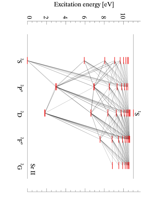
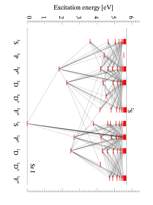
Our model of Sr is similar to that of Andrievsky et al. (2011) with respect to the term structure and the number of dipole-permitted transitions of Sr ii. However, we include more accurate transition probabilities for Sr ii. More importantly, our model atom includes new quantum-mechanical photoionization cross-sections for Sr i and e^- impact excitation cross-sections for dipole-permitted and forbidden transitions in Sr ii (see below). The model atoms employed by Short & Hauschildt (2006) and Mashonkina & Gehren (2001) are much simpler than that employed in this work ($84$ and $41$ total levels, respectively).

2.2.1 New calculations of atomic data

We compute single-electron orbitals for the target ions Sr⁺ with the atomic structure code autostructure by Badnell (1986, 1997). This code is an extension of the program superstructure (Eissner & Nussbaumer 1969), computes fine-structure CI energy levels, and radiative and Auger rates in a Breit-Pauli relativistic framework. Single electron orbitals are constructed by diagonalizing the non-relativistic Hamiltonian, within a statistical Thomas-Fermi-Dirac-Amaldi (TFDA) model potential (Eissner & Nussbaumer 1969). The scaling parameters are optimized by minimizing a weighted sum of the LS term energies. We employ a very extensive configuration expansion with configurations of the form $4p^{6}nl$, with $n$ going from 4 to 6 and $l\leq 3$, and configurations with multiple promotion from the 4p orbital, i.e. $4p^{q}5s^{r}4d^{t}nl$ with $3\leq q\leq 6$, $0\leq r\leq 2$, and $0\leq t\leq 2$. These multiple promotions from the 4p orbital are essential in computing the photoionization cross sections and that will be the subject of a future publication.

Our target representations give term energies in reasonable agreement, within $\sim 5$ percent with experimental values.

The photoionization cross-sections are computed with the R-matrix method (Burke et al. 1971). The present calculation for Sr⁰ includes the lowest $67$ LS-terms of the target in the close coupling expansion and all short range (N+1)-electron configurations that results from adding an electron to the target configurations. We find $197$ singlet and triplet bound terms of Sr⁰ with $n<9$ and $L\leq 5$, and compute photoionization cross sections for all of them. The cross sections are computed at an even energy mesh of $5\times 10^{-5}$ Ry from threshold up to 0.23 Ry, mesh of $10^{-3}$ Ry from 0.23 Ry to 2.3 Ry (roughly the highest target threshold), and another mesh of 0.02 Ry from 2.3 Ry to 4.3 Ry. Figure 2 shows the partial cross sections for ionization from the ground term of Sr⁰ into each of the first six terms of the target Sr⁺. We note, however, that DETAIL is not yet able to consistently treat ionization to specific states of the target ion. Therefore, total photoionization cross-sections are adopted here. Figure 3 shows the total cross sections for the lowest six excited state of Sr⁰. For comparison, we show the hydrogenic cross-sections computed with effective principal quantum number. The latter reproduce the functional dependence of the cross-section with energy. However, the quantum-mechanical photoionization cross-sections are typically larger both in the background (factor of two to five) and in the resonances (up to three orders of magnitude).

Figure 2: Partial photoionization cross-sections for the Sr i ground state into the lowest six states of the Sr ii target. The cross-sections are dominated by prominent resonances.

Figure 3: Total photoionization cross-sections for the selected Sr i levels. Dotted lines show hydrogenic cross-sections. The new cross-sections are up to few orders of magnitude larger than the commonly-used hydrogenic approximation.

2.2.2 Collision rates

Electron impact excitation rate coefficients for the $49$ levels of Sr ii levels were taken from Bautista et al. (2002). The data were computed with the same technique, i.e., the close-coupling approximation with the R-matrix method. For all other levels of Sr i and Sr ii the electron collision rates were computed using the formulae of van Regemorter (1962) for dipole-allowed and Allen (1973) for dipole-forbidden transitions. Cross-sections for transitions caused by inelastic collisions with H i atoms are basically unknown for any atom heavier than Mg. The only available formula developed originally for collisions between equal H-like atoms (Drawin 1968, 1969) and later slightly modified by Steenbock & Holweger (1984) and Lambert (1993) was shown to over-estimate the rates of bound-bound transitions by two to seven orders of magnitude (Belyaev & Barklem 2003; Barklem et al. 2012). Furthermore, the charge transfer processes can not be described by this simple classical formula at all. Our tests with various scaling factors to the Drawin’s H i inelastic collision cross-sections demonstrated that excitation and ionization balance of Sr i/Sr ii in the reference stars can be satisfied simultaneously only if the efficiency of H i collisions is very low (Sect. 4), few orders of magnitude lower than that given by the Drawin’s recipe, which is consistent with the quantum-mechanical results mentioned above. On these grounds we do not include inelastic H i collisions in our reference model atom.

2.3 Line selection and atomic data

In spectra of FGK stars, only a few Sr lines are useful for abundance determinations. These are two Sr i and $6$ Sr ii lines. The Sr i resonance line at $4607$ Å is weak, and, thus, sufficiently reliable for more metal-rich stars ([Fe/H]$>-1.5$) observed at high resolution. The two resonance Sr ii lines, in contrast, remain strong even in spectra of very metal-poor stars, however, severe blends in the inner and outer wings lead to systematic errors in abundances, when the blends are not properly accounted for. The three near-IR Sr ii lines at $1\mu$m appear to be un-blended and are sufficiently strong to be detected even at [Fe/H] $<-2$.

Table 1: Lines of Sr i and Sr ii selected for abundance calculations.

$\lambda$	$E_{\rm low}$	low	$E_{\rm up}$	up	$\log gf$	$\log(\gamma/N_{\rm H})$	$\log C_{6}$
$\AA$	[eV]		[eV]			rad cm3 s-1
Sr i
4607.33	0.00	${\rm 5s^{2}}\,^{1}{\rm S}_{\rm 0}$	2.69	${\rm 5p}\,^{1}{\rm P}^{{\rm\circ}}_{\rm 1}$	$0.283$	$-7.53$	$-31.2$
7070.01	1.85	${\rm 5p}\,^{3}{\rm P}^{{\rm\circ}}_{\rm 2}$	3.60	${\rm 6s}\,^{3}{\rm S}_{\rm 1}$	$-0.020$	$-7.15$	$-30.2$
Sr ii
4077.71	0.00	${\rm 5s}\,^{2}{\rm S}_{\rm 1/2}$	3.04	${\rm 5p}\,^{2}{\rm P}^{{\rm\circ}}_{\rm 3/2}$	$0.158$	$-7.81$	$-32.0$
4167.80	2.94	${\rm 5p}\,^{2}{\rm P}^{{\rm\circ}}_{\rm 1/2}$	5.92	${\rm 6s}\,^{2}{\rm S}_{\rm 1/2}$	$-0.502$	$-7.81$	$-32.0$
4215.52	0.00	${\rm 5s}\,^{2}{\rm S}_{\rm 1/2}$	2.94	${\rm 5p}\,^{2}{\rm P}^{{\rm\circ}}_{\rm 1/2}$	$-0.155$	$-7.81$	$-32.0$
10036.65	1.81	${\rm 4d}\,^{2}{\rm D}_{\rm 3/2}$	3.04	${\rm 5p}\,^{2}{\rm P}^{{\rm\circ}}_{\rm 3/2}$	$-1.194$	$-7.64$	$-31.5$
10327.31	1.84	${\rm 4d}\,^{2}{\rm D}_{\rm 5/2}$	3.04	${\rm 5p}\,^{2}{\rm P}^{{\rm\circ}}_{\rm 3/2}$	$-0.240$	$-7.64$	$-31.5$
10914.89	1.80	${\rm 4d}\,^{2}{\rm D}_{\rm 3/2}$	2.94	${\rm 5p}\,^{2}{\rm P}^{{\rm\circ}}_{\rm 1/2}$	$-0.474$	$-7.64$	$-31.5$

Table 2: Hyperfine structure and isotopic shift for the 4077 $\AA$ line.

Isotope	$\lambda$	$\log gf$
	$\AA$
87	4077.697	$-1.645$
87	4077.699	$-1.485$
84	4077.708	$-2.094$
86	4077.709	$-0.848$
88	4077.710	$0.075$
87	4077.724	$-1.465$
87	4077.725	$-1.956$

The lines selected in this work are given in Table 1. The transition probabilities were taken from different experimental and theoretical sources. According to NIST, the Sr i $gf$-values are very accurate, the uncertainty is lower than $1$ percent for the $4607$ Å line and better than $10$ percent for the $7070$ Å subordinate line. These $gf$-values are taken from the laboratory analysis of Parkinson (1976) and García & Campos (1988), respectively. The oscillator strengths of the near-IR Sr ii lines were adopted from the only available laboratory results of Gallagher (1967). These are fully consistent with the most recent ab initio calculations of Bautista et al. (2002), which are also adopted in the NLTE model atom.

Damping widths for the calculation of broadening due to elastic collisions with H i are available for the Sr ii lines from the quantum-mechanical calculations of Barklem et al. (2000) and for the Sr i lines they were kindly provided by the referee. We adopt the values from Barklem et al. for the near-IR Sr ii transitions. However, for the strong resonance Sr ii lines, which are very sensitive to this parameter, our spectrum synthesis calculations indicate somewhat lower values, by $\sim 20$ percent. The question is whether this difference can be attributed to the uncertainties of the theoretical data arising because of certain approximations in the Anstee, Barklem, and O’Mara (ABO) theory. These include representation of the interaction potential and collisional dynamics and have been investigated by Kerkeni et al. (2004) for neutral atoms of Mg, Sr, Ca, and Na. They find that whereas the semi-classical description of a collision is a sufficiently-good approximation, the ABO potentials become rather inaccurate at small interatomic separations. However, the effect of the latter is rather to under-estimate the line width that clearly does not explain our finding. For the Sr ii $4167$ line we assume the same $\gamma$ as for the resonance lines, but note that the line is too weak even in the solar spectrum to be sensitive to this parameter at all.

The adopted values of damping widths at $10000$ K per H atom, $\gamma/N_{\rm H}$, as well as the commonly-used interaction constants in the van der Waals-type interaction C₆ computed for $T=5780$ K, are given in the Table 1. Here, the latter is a parameter in the Unsöld (1955, Eq. 82,48) formula needed to reproduce the correct line width $\gamma$ at the given temperature.

For the $4077$ Sr ii line, which will be used for the abundance determinations in Sect. 4, we included the hyperfine structure and isotopic shifts. The magnetic dipole and electric quadrupole constants were taken from Buchinger et al. (1990): A (${\rm 5s^{2}}\,^{1}{\rm S}_{\rm 0}$)$=-1000.5$ MHz, A (${\rm 5p}\,^{2}{\rm P}^{{\rm\circ}}_{\rm 3/2}$) $=-36$ MHz, B (${\rm 5p}\,^{2}{\rm P}^{{\rm\circ}}_{\rm 3/2}$) $=88.5$ MHz. The data are in agreement with the older experiment by Borghs et al. (1983) and theoretical calculations by Yu et al. (2004). Isotope shifts for ⁸⁴Sr, ⁸⁶Sr, ⁸⁷Sr were taken from Borghs et al. (1983) and the solar isotopic ratios were adopted. The wavelengths and $\log gf$ values of the hyperfine structure (HFS) components are given in Table 2. We note that the 4215 Å Sr i line is only used for a comparative LTE to NLTE analysis for the reasons discussed in Sect. 3.3.

3 Statistical equilibrium of Sr

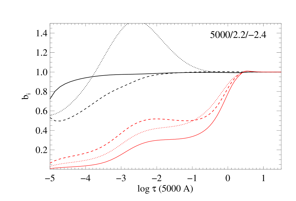
The departure coefficients for selected levels of Sr are shown as a function of continuum optical depth $\log\tau_{\rm c}$ at $500$ in Fig. 4 for the model atmospheres with parameters corresponding to dwarfs and giants with [Fe/H] $=0$ and $-2.4$. Only the levels, which give rise to the spectral lines selected for the abundance analysis (Table 1), are included in the plots. These are two levels of Sr i, forming the resonance lines at $4607$ Å, and two levels of Sr ii, which are connected by the $4077$ Å transition commonly used in the analysis of metal-poor stars.

Table 3: NLTE abundance corrections for the 4607 Sr I line.

$T_{\mathrm{eff}}$	[Fe/H]	$\Delta_{\mathrm{NLTE}}$
$\log g$		2.20	2.60	3.00	3.40	3.80	4.20	4.60
4400	$-3.0$	0.54	0.51	0.47	–	–	–	–
4400	$-2.4$	0.49	0.49	0.49	–	–	–	–
4400	$-1.2$	0.29	0.29	0.28	–	–	–	–
4400	$-0.6$	0.27	0.26	0.24	–	–	–	–
4400	$0.0$	0.19	0.18	0.16	–	–	–	–
4800	$-3.0$	0.55	0.55	0.51	0.49	0.45	–	–
4800	$-2.4$	0.50	0.51	0.51	0.49	0.46	0.43	0.36
4800	$-1.2$	0.32	0.33	0.33	0.33	0.32	0.30	0.28
4800	$-0.6$	0.17	0.17	0.18	0.18	0.17	0.16	0.14
4800	$0.0$	0.19	0.18	0.18	0.17	0.15	0.13	0.10
5200	$-3.0$	0.50	0.52	0.52	0.50	0.47	0.45	0.42
5200	$-2.4$	0.47	0.48	0.49	0.48	0.45	0.43	0.41
5200	$-1.2$	0.34	0.35	0.36	0.36	0.35	0.34	0.32
5200	$-0.6$	0.19	0.20	0.20	0.20	0.20	0.19	0.17
5200	$0.0$	0.09	0.10	0.10	0.11	0.11	0.10	0.09
5600	$-3.0$	0.44	0.45	0.46	0.46	0.45	0.42	0.40
5600	$-2.4$	0.40	0.42	0.43	0.43	0.43	0.40	0.38
5600	$-1.2$	0.31	0.32	0.33	0.33	0.33	0.32	0.31
5600	$-0.6$	0.23	0.24	0.24	0.24	0.24	0.23	0.21
5600	$0.0$	0.09	0.10	0.10	0.10	0.11	0.10	0.09
6000	$-3.0$	0.39	0.39	0.39	0.39	0.39	0.37	0.35
6000	$-2.4$	0.35	0.36	0.36	0.37	0.36	0.35	0.34
6000	$-1.2$	0.27	0.28	0.28	0.28	0.28	0.28	0.27
6000	$-0.6$	0.22	0.23	0.23	0.23	0.23	0.22	0.21
6000	$0.0$	0.14	0.14	0.14	0.14	0.13	0.13	0.12

Table 4: NLTE abundance corrections for the 4077 Sr II line.

$T_{\mathrm{eff}}$	[Fe/H]	$\Delta_{\mathrm{NLTE}}$
$\log g$		2.20	2.60	3.00	3.40	3.80	4.20	4.60
4400	$-3.9$	$-0.07$	$-0.04$	$-0.04$	–	–	–	–
4400	$-3.0$	0.00	0.00	0.00	–	–	–	–
4400	$-2.4$	0.00	0.00	0.00	–	–	–	–
4400	$-1.2$	0.00	0.00	0.00	–	–	–	–
4400	$-0.6$	0.00	0.00	0.00	–	–	–	–
4400	$0.0$	0.00	0.00	0.00	–	–	–	–
4800	$-3.9$	$-0.11$	$-0.08$	$-0.04$	$-0.01$	$-0.01$	–	–
4800	$-3.0$	$-0.02$	$-0.02$	$-0.02$	$-0.01$	$-0.01$	$-0.01$	0.00
4800	$-2.4$	0.00	0.00	0.00	0.00	$-0.01$	$-0.01$	0.00
4800	$-1.2$	0.00	0.00	0.00	0.00	0.00	0.00	0.00
4800	$-0.6$	0.00	0.00	0.00	0.00	0.00	0.00	0.00
4800	$0.0$	0.00	0.00	0.00	0.00	0.00	0.00	0.00
5200	$-3.9$	$-0.07$	$-0.03$	0.01	0.05	0.08	0.12	0.13
5200	$-3.0$	$-0.05$	$-0.06$	$-0.06$	$-0.05$	$-0.04$	$-0.03$	$-0.01$
5200	$-2.4$	$-0.01$	$-0.01$	$-0.01$	$-0.01$	$-0.01$	$-0.01$	$-0.01$
5200	$-1.2$	0.00	0.00	0.00	0.00	$-0.01$	$-0.01$	$-0.01$
5200	$-0.6$	0.00	0.00	0.00	0.00	0.00	0.00	0.00
5200	$0.0$	0.00	0.00	0.00	0.00	0.00	0.00	0.00
5600	$-3.9$	0.05	0.08	0.11	0.13	0.14	0.14	0.15
5600	$-3.0$	$-0.07$	$-0.08$	$-0.09$	$-0.08$	$-0.06$	$-0.04$	$-0.01$
5600	$-2.4$	$-0.01$	$-0.03$	$-0.03$	$-0.04$	$-0.04$	$-0.04$	$-0.03$
5600	$-1.2$	0.00	0.00	-0.01	-0.01	-0.01	-0.01	-0.01
5600	$-0.6$	0.00	0.00	0.00	-0.01	-0.01	-0.01	-0.01
5600	$0.0$	0.00	0.00	0.00	0.00	0.00	0.00	0.00
6000	$-3.9$	0.19	0.19	0.19	0.18	0.17	0.16	0.15
6000	$-3.0$	$-0.04$	$-0.06$	$-0.06$	$-0.05$	$-0.04$	$-0.02$	0.01
6000	$-2.4$	$-0.01$	$-0.03$	$-0.05$	$-0.06$	$-0.07$	$-0.07$	$-0.06$
6000	$-1.2$	0.01	0.00	$-0.01$	$-0.01$	$-0.01$	$-0.01$	$-0.01$
6000	$-0.6$	0.00	0.00	0.00	$-0.01$	$-0.01$	$-0.01$	$-0.01$
6000	$0.0$	0.00	0.00	0.00	0.00	0.00	0.00	0.00

Table 5: NLTE abundance corrections for the 10036 Sr II line.

$T_{\mathrm{eff}}$	[Fe/H]	$\Delta_{\mathrm{NLTE}}$
$\log g$		2.20	2.60	3.00	3.40	3.80	4.20	4.60
4400	$-3.9$	$-0.14$	$-0.15$	$-0.18$	–	–	–	–
4400	$-3.0$	$-0.13$	$-0.12$	$-0.12$	–	–	–	–
4400	$-2.4$	$-0.13$	$-0.12$	$-0.12$	–	–	–	–
4400	$-1.2$	$-0.17$	$-0.15$	$-0.13$	–	–	–	–
4400	$-0.6$	$-0.15$	$-0.14$	$-0.13$	–	–	–	–
4400	$0.0$	$-0.10$	$-0.11$	$-0.10$	–	–	–	–
4800	$-3.9$	$-0.18$	$-0.18$	$-0.19$	$-0.20$	$-0.12$	–	–
4800	$-3.0$	$-0.13$	$-0.13$	$-0.12$	$-0.12$	$-0.12$	$-0.09$	$-0.08$
4800	$-2.4$	$-0.15$	$-0.14$	$-0.13$	$-0.12$	$-0.10$	$-0.09$	$-0.05$
4800	$-1.2$	$-0.19$	$-0.17$	$-0.15$	$-0.12$	$-0.09$	$-0.07$	$-0.06$
4800	$-0.6$	$-0.17$	$-0.16$	$-0.14$	$-0.12$	$-0.09$	$-0.07$	$-0.05$
4800	$0.0$	$-0.11$	$-0.12$	$-0.11$	$-0.10$	$-0.08$	$-0.07$	$-0.05$
5200	$-3.9$	$-0.19$	$-0.19$	$-0.19$	$-0.19$	$-0.17$	$-0.15$	$-0.13$
5200	$-3.0$	$-0.13$	$-0.12$	$-0.12$	$-0.12$	$-0.11$	$-0.10$	$-0.09$
5200	$-2.4$	$-0.14$	$-0.14$	$-0.13$	$-0.12$	$-0.10$	$-0.09$	$-0.08$
5200	$-1.2$	$-0.20$	$-0.19$	$-0.16$	$-0.13$	$-0.10$	$-0.08$	$-0.06$
5200	$-0.6$	$-0.19$	$-0.18$	$-0.16$	$-0.13$	$-0.10$	$-0.07$	$-0.05$
5200	$0.0$	$-0.13$	$-0.13$	$-0.12$	$-0.11$	$-0.09$	$-0.07$	$-0.05$
5600	$-3.9$	$-0.16$	$-0.15$	$-0.14$	$-0.12$	$-0.10$	$-0.06$	$-0.03$
5600	$-3.0$	$-0.10$	$-0.10$	$-0.10$	$-0.10$	$-0.09$	$-0.07$	$-0.05$
5600	$-2.4$	$-0.12$	$-0.11$	$-0.10$	$-0.09$	$-0.08$	$-0.07$	$-0.06$
5600	$-1.2$	$-0.20$	$-0.19$	$-0.17$	$-0.14$	$-0.11$	$-0.08$	$-0.06$
5600	$-0.6$	$-0.19$	$-0.19$	$-0.17$	$-0.15$	$-0.12$	$-0.08$	$-0.06$
5600	$0.0$	$-0.14$	$-0.14$	$-0.14$	$-0.13$	$-0.11$	$-0.08$	$-0.06$
6000	$-3.9$	$-0.08$	$-0.06$	$-0.04$	$-0.02$	$0.01$	$0.04$	$0.07$
6000	$-3.0$	$-0.06$	$-0.06$	$-0.05$	$-0.05$	$-0.03$	$-0.02$	$0.01$
6000	$-2.4$	$-0.08$	$-0.07$	$-0.06$	$-0.06$	$-0.05$	$-0.04$	$-0.03$
6000	$-1.2$	$-0.17$	$-0.16$	$-0.14$	$-0.12$	$-0.10$	$-0.08$	$-0.06$
6000	$-0.6$	$-0.18$	$-0.18$	$-0.17$	$-0.15$	$-0.12$	$-0.09$	$-0.06$
6000	$0.0$	$-0.14$	$-0.15$	$-0.14$	$-0.14$	$-0.12$	$-0.09$	$-0.07$

3.1 NLTE effects in Sr i

Figure 4: Departure coefficients $b_{i}$ of selected Sr i and Sr ii levels for different stellar parameters, $T_{\rm eff}$, $\log g$, and [Fe/H] (indicated in each sub-plot). Red: Sr i levels, ${\rm 5s^{2}}\,^{1}{\rm S}$ (solid), ${\rm 5p}\,^{3}{\rm P}^{{\rm\circ}}$ (dotted), ${\rm 5p}\,^{1}{\rm P}^{{\rm\circ}}$ (dashed). Black: Sr ii levels, ${\rm 5s}\,^{2}{\rm S}_{\rm 1/2}$ (solid), ${\rm 4d}\,^{2}{\rm D}_{\rm 3/2}$ (dotted), ${\rm 5p}\,^{2}{\rm P}^{{\rm\circ}}_{\rm 1/2}$ (dashed).

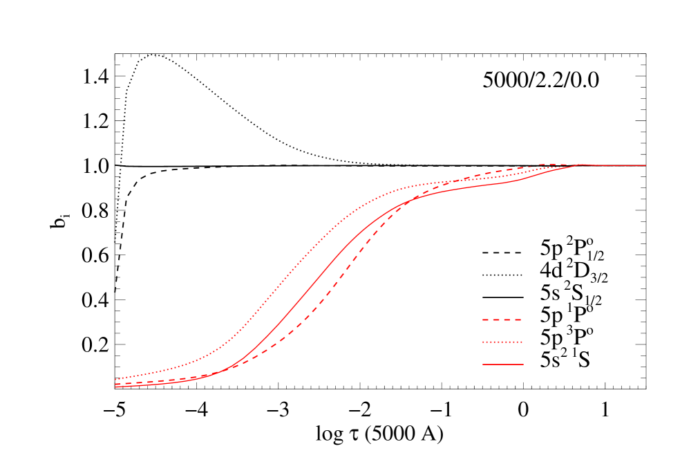
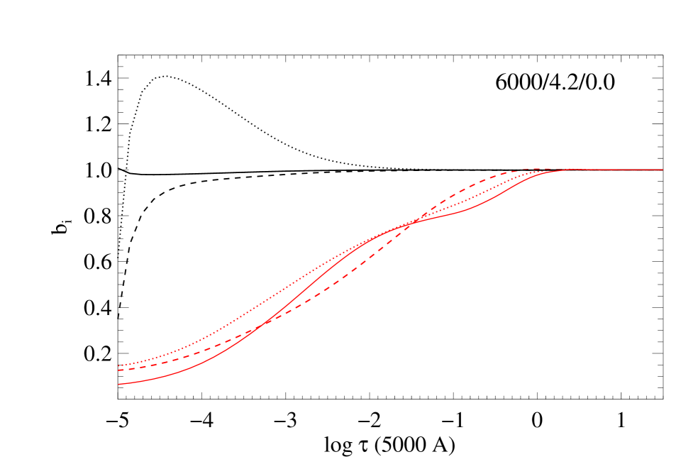
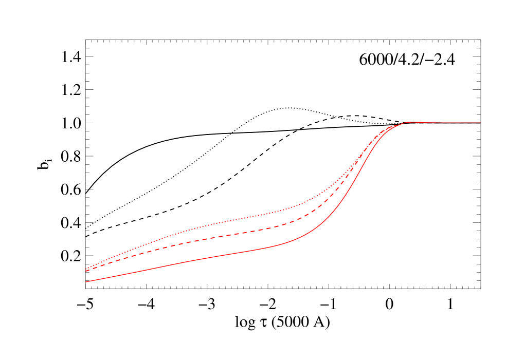
Sr i with the ionization potential $5.69$ eV is a trace atom in the the atmospheres of late-type stars. The ratio of Sr i/Sr ii falls below $10^{-3}$ above continuum optical depth unity, and the departures from LTE in the distribution of atomic level populations are almost entirely due to overionization. The behavior of the Sr i departure coefficients with stellar parameters, thus, resembles that of the similar trace atoms, such as Co i (Bergemann et al. 2010) or Cr i (Bergemann & Cescutti 2010). The levels are underpopulated and their $b_{i}$-factors monotonously decrease outwards. The ground state ${\rm 5s^{2}}\,^{1}{\rm S}$ with the ionization edge at $2177$ Å is also strongly over-ionized and it decouples from the other low-excited levels because collisions can not bridge the large energy gap of $\sim 2$ eV between them. Line transitions have a small influence on the statistical equilibrium of Sr i causing some changes of the level populations only in the solar-metallicity models. For example, in the metal-rich models (Fig. 4, left panel), the departure coefficient of the 5p $\@element[1]{\mathrm{P^{o}}}$ level drops below that of the 5s² $\@element[1]{\mathrm{S}}$ at $\log\tau_{\rm c}\approx-1$, marking the depth at which the $4607$ resonance line becomes optically thin, and spontaneous transitions depopulate the upper level of the transition.

In the metal-poor models (Fig. 4, right panel), the coupling of the levels by radiative bound-bound transitions and collisions diminishes even though the collision rates between the low-excited levels are large enough to keep them are in detailed balance even in the models with [Fe/H] $=-1$. The populations are now set primarily by the balance between radiative ionizations and recombinations, and the run of $b_{i}$-factors with $\log\tau_{\rm c}$ simply reflects the mean intensity vs Planck function inequalities, $J_{\nu}\neq B_{\nu}$, at the frequencies of the level photoionization continua at each depth point. For example, in the model with $T_{\rm eff}=6000$ K, $\log g=4.2$, and [Fe/H] $=-2.4$, the lowest energy levels 5p $\@element[3]{\mathrm{P^{o}}}$ and 5p $\@element[1]{\mathrm{P^{o}}}$ decouple from each other and from the continuum at $\log\tau_{\rm c}\approx 0$. Then, in a very narrow interval of optical depths, $-1<\log\tau_{\rm c}<0$, their departure coefficients demonstrate a sudden drop following the steep temperature gradient of the atmosphere, and thus, rapidly increasing $J_{\nu}-B_{\nu}$ imbalance (note that matter becomes transparent to the radiation above ionization edges of both levels, $3202$ and $4126$ Å at $\log\tau_{\rm c}=+0.11$ respectively $\log\tau_{\rm c}=+0.05$). Further out, $\log\tau_{\rm c}<-1$, where the mean intensity as well as the local kinetic temperature remain roughly constant, the departure coefficients smooth out, slowly decreasing outwards.

The NLTE effects on the formation of the Sr i line at $4607$ Å are generally to decrease the line opacity, shifting the line $\tau_{\nu}$ scale to the deeper hotter atmospheric layers and, thus, leading to weaker lines compared to the LTE case.

3.2 NLTE effects in Sr ii

The NLTE effects on the Sr ii levels are due to the non-equilibrium excitation in the line transitions. This was extensively investigated by Belyakova & Mashonkina (1997) and Short & Hauschildt (2006), and our results are qualitatively very similar to these studies. The analysis of radiative and collisional rates populating and de-populating the levels, as well as trial calculations with atomic models devoid of some key transitions, in particular the resonance and subordinate lines, allows us to draw the following conclusions.

In the solar-metallicity models (Fig. 4, left panel), the ground state, ${\rm 5s}\,^{2}{\rm S}$ ($\lambda_{\rm thr}\sim 1130\AA$) and the lowest odd level ${\rm 5p}\,^{2}{\rm P}^{{\rm\circ}}$ level ($\lambda_{\rm thr}\sim 1540\AA$ , $E\sim 3$ eV) have nearly LTE populations out to $\log\tau_{\rm c}\sim-3$, and become underpopulated only in the outermost layers, which are transparent to the radiation across their ionization edges. Still, there is small net radiative excitation in the transitions from these levels upwards, which very efficiently populates the levels with excitation energy $E\geq 6$ eV, such as ${\rm 5d}\,^{2}{\rm D}$, ${\rm 6p}\,^{2}{\rm P}^{{\rm\circ}}$, and ${\rm 7s}\,^{2}{\rm S}$ (not shown in the plots) due to their small Boltzmann factors. The high-excited levels are, however, also over-ionized, which in turn, increases the number density of the Sr iii ground state. The lowest metastable Sr ii level ${\rm 4d}\,^{2}{\rm D}$ ($E\sim 1.8$ eV) is nearly in thermal equilibrium with ${\rm 5p}\,^{2}{\rm P}^{{\rm\circ}}$ due to the dominance of collision rates in the deeper layers, however in the outer layers it gains appreciable overpopulation due to the photon losses in the near-IR transitions between the two levels. In fact, this process is a part of photon suction in a sequence of low-frequency transitions, which connect ${\rm 4d}\,^{2}{\rm D}$ to a large number of high-levels close to the continuum. Many of these transitions become optically thin at $\log\tau_{\rm c}<-3$, so that spontaneous de-excitation lead to the overpopulation ${\rm 4d}\,^{2}{\rm D}$, the lowest energy state of the cascading sequence.

The departures from LTE change with decreasing metallicity (Fig. 4, right panel). First, the line transitions weaken and and over-population of ${\rm 4d}\,^{2}{\rm D}$ occurs in the deeper layers compared to the solar metallicity models. Also, radiative pumping in the resonance transitions at $4077$ and $4215$ Å is more efficient due to larger radiative fluxes. This process leads to a marked over-population of the ${\rm 5p}\,^{2}{\rm P}^{{\rm\circ}}$ level at $-1<\log\tau_{\rm c}<0$, especially in the hotter model, $T_{\rm eff}=6200$ K. Outside these optical depths, over-ionization dominates and all low-lying levels become underpopulated. The importance of strong line scattering was tested by excluding the resonance lines and subordinate lines at $1$ $\mu$m from the model atom. The overpopulation of the ${\rm 5p}\,^{2}{\rm P}^{{\rm\circ}}$ and ${\rm 4d}\,^{2}{\rm D}$ vanished both for the metal-rich and metal-poor models.

Figure 5: NLTE abundance corrections for the Sr i and Sr ii lines. Note different x-axis scales.

3.3 NLTE abundance corrections

To quantify the effect of NLTE on the abundance determinations, we use the concept of the NLTE abundance correction $\Delta_{\rm NLTE}$, where:

$$\Delta_{\rm NLTE}=\log\epsilon\rm{(Sr)}_{\rm NLTE}-\log\epsilon\rm{(Sr)}_{\rm LTE}$$ (1)

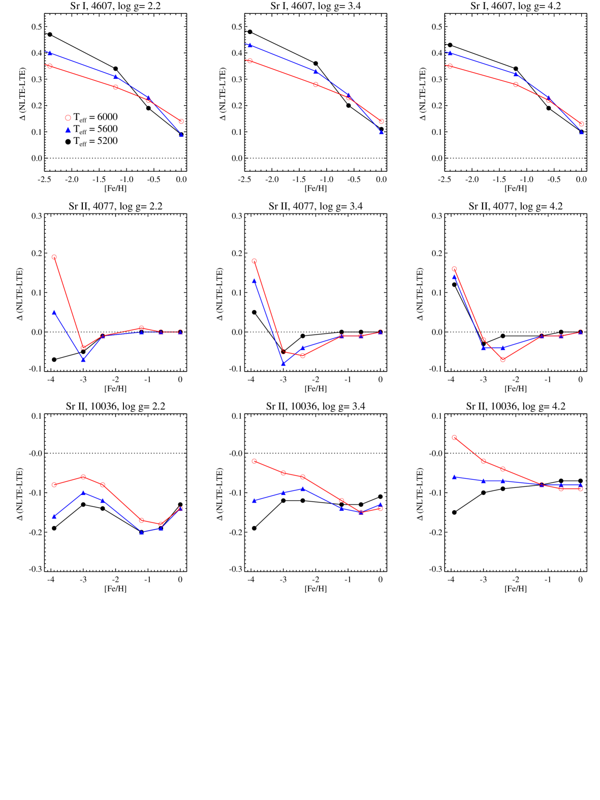
is the the logarithmic correction, which has to be applied to an LTE abundance determination of a specific line to obtain the exact value corresponding to the use of NLTE line formation. These values were computed for a grid of model atmospheres by equalizing the NLTE equivalent widths though varying the element abundance in the LTE calculations. The NLTE abundance corrections for the $4077$, $4607$ and $10036$ line are given in Tables 3, 4, and 5 for a wide range of stellar parameters. Fig. 5 (top panel) also shows the values of $\Delta_{\rm NLTE}$ for selected model atmospheres as a function of effective temperature, gravity, and [Fe/H].

As evident from Fig. 5 (top panel) and Table 3, the NLTE abundance corrections for the $4607$ Å are always positive, and they are maximum for cool giants with sub-solar metallicity, [Fe/H] $<-1$. This behavior can be easily understood by inspecting the plots of departure coefficients (Fig. 4, top right panel): at the typical depths of the resonance line formation, $\log\tau_{\rm c}\sim 0...-0.5$, the level populations are already depleted by a factor of two compared to LTE. In the models of warmer metal-poor dwarfs, the line formation is confined to the deeper layers, $\log\tau_{\rm c}\sim 0$, where the NLTE effects in the Sr i ionization balance are smaller. This is reflected in the behavior of the abundance corrections, which also decrease. $\Delta_{\rm NLTE}$ are comparatively small for the warmest models, corresponding to horizontal branch stars ($T_{\rm eff}=6200$ and $\log g=2.2$). Note, however, that at $T_{\rm eff}>6000$ K and [Fe/H]$<-1.5$ the $4607$ Å line is very weak, $W_{\lambda}<0.5$ mÅ, and, thus, is not useful for abundance determinations. In contrast, the line could be suitable for the analysis in sufficiently good-quality (R $>$ 20000, S/N $>$50) spectra of giants and sub-giants down to [Fe/H] $\sim-2.5$.

As described in the previous section, the formation of Sr ii lines is also significantly affected by the NLTE effects. Inspection of Table 4 and Fig. 5 (middle panel) shows that for the resonance Sr ii line at $4077$ Å the NLTE abundance corrections are typically negative for stars with metallicity [Fe/H]$>-3$, but rapidly increase for more metal-poor stars with $T_{\rm eff}>5000$ K and/or $\log g>3$. The amplitude of $\Delta_{\rm NLTE}$ increases with $T_{\rm eff}$ and decreasing $\log g$. Another resonance Sr ii line at $4215$ Å shows the same pattern and the NLTE abundance corrections are nearly identical; we caution, however, that this line is blended by an Fe i line, and should be avoided in abundance analyses of cool stars. The implication is that, compared to NLTE, traditional LTE studies relying on the resonance Sr ii lines under-estimate the abundance of Sr in very metal-poor stars, but somewhat over-estimate it for less metal-poor objects, such at that of thick and thin disk of the Galaxy.

For the near-IR subordinate Sr ii lines, the NLTE abundance corrections are typically negative (Table 5 and Fig. 5, bottom panel), being as large as $-0.2$ dex even for mildly metal-poor giants; this behaviour is consistent with the discussion in Sect. 3.2, as the NLTE effects are due to strong line scattering. However, $\Delta_{\rm NLTE}$ are usually within $-0.1$ dex for dwarfs and become mildly positive only at very low metallicity, [Fe/H] $<-3$ and $T_{\rm eff}>6000$ K. The NLTE abundance corrections presented in Table 5 are rather similar for the other two members of the near-IR triplet, i.e., the lines at $10327$ and $10914$ Å, and can be provided by request.

Our NLTE abundance corrections are in line with the results of Short & Hauschildt (2006), although they investigated the formation of the resonance Sr ii lines only. They find NLTE line strengthening for the giant models with [Fe/H] $=-1\ldots-2$ and NLTE weakening for the models with [Fe/H] $=-4\ldots-5$. However, we note some qualitative differences with Andrievsky et al. (2011). For example, for the near-IR Sr ii lines their abundance corrections at [Fe/H] $=-3$ and $T_{\rm eff}=4800-5300$ K are of the order of $-0.3$ to $-0.5$ dex and are very sensitive to surface gravity (their Fig. 7, top panel). In contrast, our values for the $10036$ Å line remain within $\sim-0.1$ dex for any $\log g$ value in this [Fe/H] and $T_{\rm eff}$ range. For the resonance Sr ii line at $4077$ Å, our $\Delta_{\rm NLTE}$ are mildy negative for any $\log g$ and $T_{\rm eff}$ at [Fe/H] $=-3$, whereas Andrievsky et al. (2011) obtain large positive corrections for dwarfs and negative $\Delta_{\rm NLTE}$ for giants. The differences are most likely caused by the differences in the NLTE model atoms, as described in Sect. 2.2.

4 Application to the abundance analysis of late-type stars

Figure 6: NLTE and LTE line-by-line Sr abundances for the selected stars. In contrast to LTE (red open circles), the Sr i and Sr ii lines provide consistent abundances in NLTE (black filled circles).

In addition to the Sun, three other late-type stars were selected for the abundance analysis. The principle selection criteria were that stellar parameters are well-constrained by independent techniques (interferometry, parallaxes), observations cover a large wavelength interval and their quality is very high for the 4607 Sr i line and the near-IR Sr ii triplet to be accurately measured. Stellar parameters for the warm turn-off star Procyon, moderately metal-poor giant Arcturus (HD 124897), and very metal-poor giant HD 122563 were taken from Korn et al. (2003), Tsuji (2009), and Mashonkina et al. (2008), respectively (Table 6). The accuracy of these parameters was verified in our recent analysis of Fe NLTE statistical equilibrium with mean 3D model atmospheres (Bergemann et al. 2012). We stress that it is not our goal here to obtain Sr abundances for a large sample of stars, as this will be the focus of our forthcoming publications (Hansen et al. in prep., Ruchti et al. in prep.), but rather to test the performance of the new NLTE model atom.

For the spectrum synthesis (Sect. 2.1), we used the solar KPNO flux spectrum (Kurucz et al. 1984). The spectra of Arcturus (HD 124897), Procyon (HD 61421), and HD 122563 were retrieved from the UVESPOP database (Bagnulo et al. 2003). These UVES (VLT, Paranal) spectra have a slit-determined resolution of $\sim 80000$ and a signal-to-noise ratio $S/N\sim 300$ near 5000 Å.

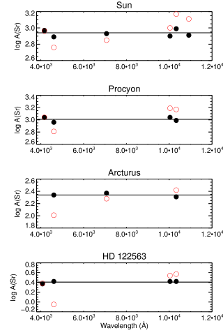
The solar abundance was determined using five Sr lines from the Table 1, adopting $T_{\rm eff}=5777$, $\log g=4.44$, [Fe/H] $=0$, and $\xi_{\rm t}=1$ km/s. The results are largely discrepant in LTE: $\log\epsilon_{\rm SrI}=2.81\pm 0.06$ and $\log\epsilon_{\rm SrII}=3.06\pm 0.1$. The NLTE model atom successfully eliminates this problem. The abundances from the two ionization stages are fully consistent $\log\epsilon_{\rm SrI}=2.91\pm 0.03$ and $\log\epsilon_{\rm SrII}=2.94\pm 0.04$ in NLTE. Here, the error corresponds to one standard deviation of the line sample. The NLTE result is also in agreement with the meteoritic abundance of Sr, $\log\epsilon=2.90\pm 0.03$ dex (Lodders et al. 2009). We note that the meteoritic abundance of Sr given by Asplund et al. (2009), Sr, $\log\epsilon=2.88\pm 0.03$ dex, is slightly lower, which is a consequence of different reference Si abundances. The solar Sr abundance was also determined by Barklem & O’Mara (2000), Andrievsky et al. (2011), and Mashonkina & Gehren (2001). The last two references perform NLTE calculations, which are generally in agreement with our results, both in terms of NLTE abundance corrections and absolute abundances. We caution, however, that this agreement is not particularly telling, because other parameters in the modeling are different. Mashonkina & Gehren (2001) adopted $\xi_{\rm t}=0.8$ km/s and employed the older (ODF) version of the MAFAGS model atmospheres. Barklem & O’Mara (2000) recover meteoritic Sr abundance from the neutral Sr lines even in LTE, which is not unexpected as they used $\xi_{\rm t}=0.85$ km/s and the solar Holweger-Müller (1974) model atmosphere.

Table 6: Basic parameters and the Sr abundances for the selected stars.

Star	Teff	$\log g$	[Fe/H]	$\xi$	LTE		NLTE
	K	(cgs)		km/s	[Sr i/Fe]	[Sr ii/Fe]	[Sr i/Fe]	[Sr ii/Fe]
HD 61421	6510	3.96	$-0.03$	1.8	$-0.08$	$0.27$	0.07	0.15
HD 122563	4600	1.60	$-2.50$	1.8	$-0.47$	$0.08$	$0.00$	$-0.02$
HD 124897	4300	1.50	$-0.50$	1.5	$-0.28$	$0.00$	$-0.07$	$-0.11$

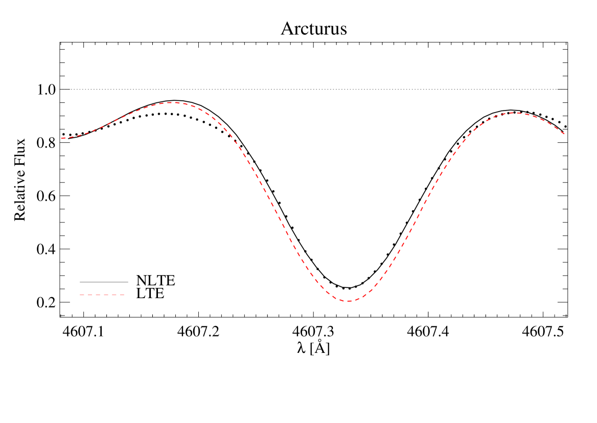
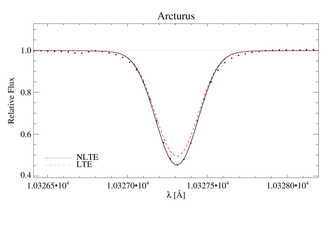
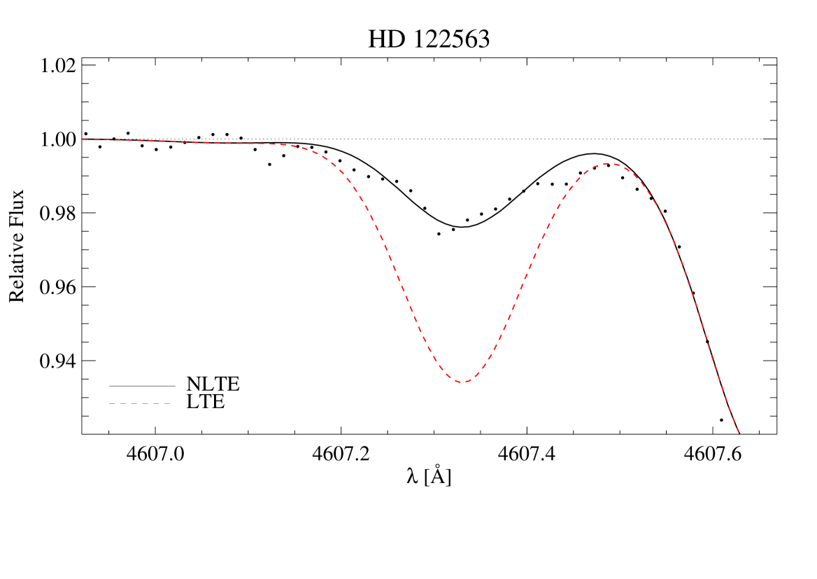
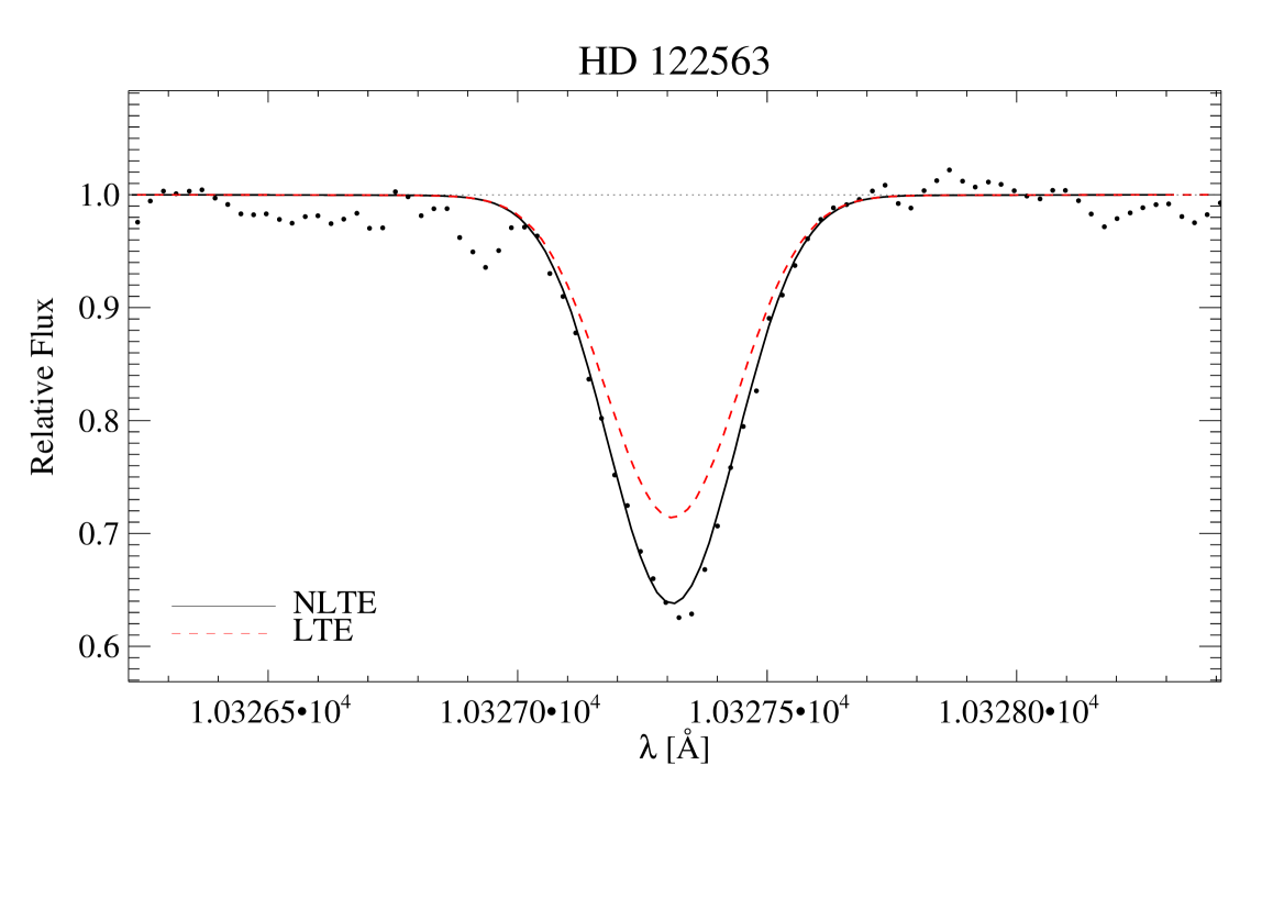
The LTE and NLTE Sr abundances determined for the reference stars are given in Table 6 and a line-by-line comparison is shown in Fig. 6. Few examples of synthetic and observed line profiles are shown in Fig. 7. Comparison of the [Sr i/Fe] and [Sr ii/Fe] from Table 6 reveals that the LTE approach predicts a systematic discrepancy between the lines of two ionization stages, which is also evident from the Fig. 6. The difference between the Sr i and the near-IR Sr ii lines, which are almost insensitive to damping, is of the order $0.3$ to $0.5$ dex. This is far beyond the uncertainties in stellar parameters, which are $\sim 80$ K for $T_{\rm eff}$, $0.1$ dex for $\log g$, and $0.1$ dex for [Fe/H]. Also, the uncertainties of the transition probabilities are far smaller than that (Sect. 2.3).

The NLTE model atom provides, in contrast, realistic ionization balance, significantly reducing the scatter between the Sr lines of different ionization stages and excitation energies (Fig. 6). In this respect, especially important is a good agreement between the NLTE abundances from the near-IR Sr ii and visual resonance Sr i line, which are very sensitive to NLTE and the effects are of different nature, i.e., overionization-stipulated decrease of opacity in the $4607$ line and source function depletion in the lines of the $1\mu$m triplet.

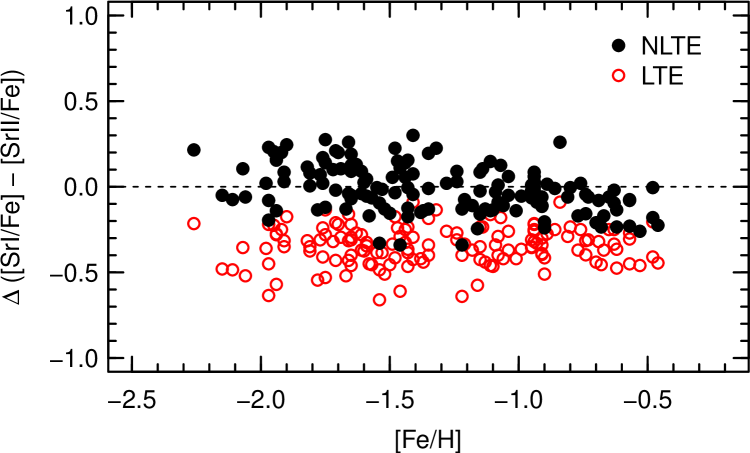
The analysis of a larger sample of stars supports the importance of NLTE effects in the ionization balance of Sr. This is evident from Fig. 8, which shows the difference between the mean abundances computed using the Sr i and Sr ii lines for a sample of thick-disk and halo RAVE stars with high-resolution spectroscopic follow-up observations (see Ruchti et al. 2011). In LTE, the mean offset between the two ionization stages is $\sim 0.4$ dex and it is alleviated when the NLTE effects are taken into account. A detailed analysis of the data will be presented in Ruchti et al. (in prep.).

We thus conclude that NLTE must be taken into account in abundance analysis of resonance Sr i and subordinate Sr ii lines in spectra of late-type stars. Also, at low metallicities, the resonance Sr ii lines are sensitive to NLTE effects, and abundances determined in LTE are largely under-estimated. It is also important to note that the NLTE effects for Sr might be larger than our estimates, because of interlocking with NLTE-affected lines of other atoms, as demonstrated by Short & Hauschildt (2006).

Figure 7: NLTE and LTE line profiles of the Sr i and Sr ii lines for selected stars compared with observed stellar spectra.

Figure 8: NLTE and LTE abundance differences between Sr i and Sr ii lines for the representative sample of thick-disk and halo stars from Ruchti et al. (2011).

5 Conclusions

We investigate statistical equilibrium of Sr in the atmospheres of late-type stars. The NLTE model atom was constructed using new atomic data, computed with the R-matrix method, which include levels, transition probabilities, photoionization and electron-impact excitation cross-sections.

The NLTE effects are significant for the Sr i resonance line at $4607$ Å and are stipulated by overionization. For the resonance Sr ii lines, typically observed in metal-poor FGK stars, our model predicts small deviations from LTE, although NLTE effects become important at very low metallicity, [Fe/H] $<-3$, reaching $+0.2$ dex for very metal-poor turnoff stars. The near-IR Sr ii triplet shows substantial sensitivity to NLTE, and the NLTE corrections vary between $+0.1$ and $-0.2$ dex depending on the model metallicity, temperature, and surface gravity.

The NLTE model atom was applied to the analysis of the Sun and three stars with well-constrained stellar parameters. In contrast to LTE approach, the NLTE model recovers ionization and excitation equilibria of Sr for all these reference stars, thus confirming that the NLTE modeling approach developed in this work provides a solid base for future abundance determinations of late-type stars.

The NLTE abundance corrections are provided for the important diagnostic Sr i and Sr ii lines for a grid of model atmospheres in the following range of stellar parameters $4400\leq T_{\rm eff}\leq 6000$ K, $2.2\leq\log g\leq 4.6$, $-4\leq$ [Fe/H] $\leq 0$; for other Sr lines and other models the abundance corrections can be also computed by request.