Encounter times in overlapping domains: application to epidemic spread in a population of territorial animals

Abstract

We develop an analytical method to calculate encounter times of two random walkers in one dimension when each individual is segregated in its own spatial domain and shares with its neighbor only a fraction of the available space, finding very good agreement with numerically-exact calculations. We model a population of susceptible and infected territorial individuals with this spatial arrangement, and which may transmit an epidemic when they meet. We apply the results on encounter times to determine analytically the macroscopic propagation speed of the epidemic as a function of the microscopic characteristics: the confining geometry, the animal diffusion constant, and the infection transmission probability.

The spatial propagation of an epidemic in a population is highly dependent on the transmission dynamics, in particular, the frequency of encounters between individuals, or contact rate, and the probability of transmission upon encounter Diekmann and Heesterbeek (2000). These, in turn, are affected by individual mobility Belik et al. (2011), by spatial structure of the environment Hufnagel et al. (2004), and by what is transmitted, e.g., an infection, a rumor, or information, which influences the contact network via which the epidemic spreads Barrat et al. (2008).

Recent studies on the importance of individual-level processes on disease propagation have reemphasized the need to develop models that go beyond the assumptions of well-mixed, homogeneous populations Ferguson et al. (2003); Colizza and Vespignani (2007); Aparicio and Pascual (2007); Aparicio and Vespigani (2011), and to link ‘macroscopic’ features of the spatial spread of an infection to ‘microscopic’ characteristics of the agents carrying the infection. In this Letter, we make a considerable advance in that direction by focusing on the role that the spatial organization of a population plays for the spread of an epidemic through that population. We relate the propagation speed of the epidemic to pairwise interaction events, consisting of direct encounters between one susceptible and one infected individual.

The rate of encounters between individuals has previously been analyzed when different individuals occupy the same spatial region Sanders and Larralde (2008); Sanders (2009); Tejedor et al. (2011), based upon recent theoretical developments on first-passage times Redner (2001) in confined geometries Condamin et al. (2007); Bénichou et al. (2010); Meyer et al. (2011). Here, we develop a framework to study encounter times when the regions occupied by individuals are distinct.

Model:-

Individuals are modeled as random walkers confined to regions of equal size; a fraction of each region overlaps those of the neighboring individuals. This spatial arrangement is common in territorial animals: individuals are confined within a home range Giuggioli et al. (2006), having exclusive access to certain core areas, the territories, Giuggioli et al. (2011), but also sharing other regions, the home-range overlap, with their neighbors.

When a population is arranged spatially, as depicted in Fig. 1, on a one-dimensional (1D) lattice, infection spread proceeds by contact between one infected individual and its neighbor; encounters may take place only within the corresponding overlap region. To represent an SI (susceptible–infected) model, we suppose that, upon encounter, transmission of the infection takes place with probability $p$.

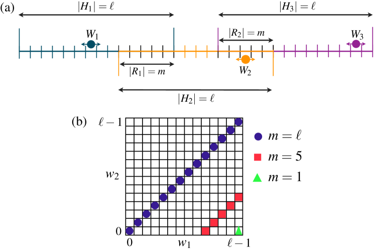
Figure 1: (Color online) (a) Three discrete random walkers, with positions $W_{i}$ on a one-dimensional lattice, in their respective habitats $H_{i}$, having overlap regions $R_{i}$ with their neighbors. (b) Mapping of $W_{1}$ and $W_{2}$ to shifted coordinates $(w_{1},w_{2})$ of a single 2D walker. Static targets corresponding to the locations where the two walkers meet are shown for $m=5$ (squares), $m=1$ (triangles) and $m=\ell$ (circles).

The discrete position of the $i$th individual is denoted by $W_{i}$; it is restricted to its home range region $H_{i}$ by reflecting boundaries, and has overlap regions $R_{i-1}$ and $R_{i}$ with, respectively, its left and right neighbor. The sizes of both types of region are constant: the $H_{i}$ each occupy $\ell$ sites, and the $R_{i}$ occupy $m$ sites. A similar geometry has been used independently in a model for heat conduction in 1D systems Ryals and Young (2012); Huveneers (2011).

Encounter times:-

We first suppose that the probability $p$ of transmission is $1$. To calculate the mean first-encounter time (MFET) between the two walkers, we map their movement onto that of a single random walker in 2D, whose allowed positions are represented by the vector $\vec{w}=(w_{1},w_{2})$; see Fig. 1(b). Here, $w_{i}:=W_{i}-(i-1)\Delta$ is the displacement of walker $i$ from the leftmost site of its habitat $H_{i}$, with $0\leq w_{i}\leq\ell-1$, and $\Delta:=\ell-m$ is the distance between the centers of $H_{i}$ and $H_{i+1}$, i.e., the mean spacing between walkers.

The possible locations where the two walkers may encounter one other then become a sequence of static target positions on the 2D lattice. When $m=1$, the overlap region is a single site, giving a single target in 2D at the bottom right corner, $(\ell-1,0)$. As $m$ increases, the target set grows, until the limiting case $m=\ell$, when the two walkers occupy the same space and the target set is the main diagonal; see Fig. 1(b).

The first-encounter time is now equivalent to the first-passage time to the 2D target set, with reflecting boundary conditions at the outer edge of Fig. 1(b). To compute this, it is convenient to consider a symmetrized version of the problem: instead of reflecting a walker which attempts to leave the domain, it is allowed to move unimpeded into a reflected copy of the domain. Doing this for all borders gives rise to an unfolded version of the system. This unfolding, a well-known technique in other fields Chernov and Markarian (2006), creates an inner absorbing rhombus inside an outer reflecting square as shown in Fig. 2(a–b).

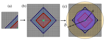
Figure 2: (Color online) Unfolding for $\ell=15$: (a) original system with reflecting boundaries; (b) unfolded system. Filled, colored sites show targets for the 2D walker for $m=1$, $m=7$ and $m=12$, shown by triangles, squares, and circles, respectively. (c) Approximation for $m=12$, replacing the region between the inner rhombus and outer square by an annulus with inner radius $a$ and outer radius $b$.

When $m=1$, the extended system has a “thick” target, i.e., four neighboring sites at the center of the lattice, while for other values of $m$ a larger rhombus of target sites is obtained. In the continuum limit, we may approximate the first-encounter distribution of the walkers by computing the first-passage distribution to the target rhombus.

When the 2D walker starts inside the rhombus, corresponding to $W_{1}>W_{2}$, i.e., walker $W_{1}$ to the right of $W_{2}$ inside their mutual overlap region, one writes the solution of the 2D diffusion equation for the probability distribution $P_{\mathrm{in}}(x,y,t)$ in Cartesian coordinates with $x$ and $y$ parallel to the edges of the rhombus and with Dirichlet (absorbing) boundary conditions, since any encounter event corresponds to the arrival at a target, when the movement process terminates.

The exact solution of this problem with a delta initial condition was obtained in ref. Tejedor et al. (2011), in terms of a double infinite series, with each series associated to one of the two orthogonal directions. Uniform initial conditions $P_{\mathrm{in}}(x,y,0)=1/L^{2}$ in our problem, where $L=m\sqrt{2}$, correspond to integrating Eq. (12) of ref. Tejedor et al. (2011) over the domain. From that expression it is straightforward to calculate the survival probability $S_{\mathrm{in}}(t)=\int_{0}^{L}dx\int_{0}^{L}dy\,P_{\mathrm{in}}(x,y,t)$, and finally the first-passage probability density $F_{\mathrm{in}}(t)=-dS_{\mathrm{in}}(t)/dt$, as

$$F_{\mathrm{in}}(t)=\frac{16}{\pi^{2}}\frac{D}{L^{2}}\sum_{\begin{subarray}{c}j\textrm{ odd},\,k\textrm{ odd}\end{subarray}}^{\infty}\left(\textstyle\frac{1}{j^{2}}+\frac{1}{k^{2}}\right)e^{-\left(j^{2}+k^{2}\right)\pi^{2}Dt/L^{2}}.$$ (1)

The mean first-encounter time is then $\int_{0}^{\infty}t\,F_{\mathrm{in}}(t)\,dt$, giving

$$\left\langle\tau_{\mathrm{enc}}\right\rangle_{\mathrm{in}}=m^{2}\left\{\frac{2}{3}-\frac{128}{\pi^{5}}\sum_{k\textrm{ odd }}^{\infty}\frac{\tanh\left[\frac{k\pi}{2}\right]}{k^{5}}\right\}=:Cm^{2},$$ (2)

valid for uniform initial conditions inside the rhombus, where the diffusion coefficient $D=\frac{1}{4}$, and so $C\simeq 0.2116$.

When the 2D walker instead starts outside the rhombus, it moves in a much more complicated geometry, and in addition the problem now has mixed boundary conditions. Since this intrinsically two-dimensional eigenvalue problem seems impossible to solve analytically, we replace the true geometry by an annulus bounded by two concentric circles, as shown in Fig. 2(c): one absorbing, of area equal to that of the inner rhombus, and hence radius $a=m\sqrt{2/\pi}$, with Dirichlet boundary condition $P_{\mathrm{out}}|_{r=a}=0$, where $r$ is the radial coordinate, and one reflecting, with area equal to that of the outer square, and so radius $b=2\ell/\sqrt{\pi}$, with no-flux (Neumann) boundary condition $\partial P_{\mathrm{out}}/\partial r|_{r=b}=0$.

We now seek the radially-symmetric solution $P_{\mathrm{out}}(r,t)$ of the diffusion equation in this annulus. For reasons arising from the epidemic spread problem below, we take uniform initial conditions inside an annulus $c\leq r\leq b$, for some $c\geq a$. Using separation of variables in the radially symmetric diffusion equation, one can determine the probability of occupation $P_{\mathrm{out}}(r,t)$ Crank (1975), the survival probability $S_{\mathrm{out}}(t)=\int_{a}^{b}r\,P_{\mathrm{out}}(r,t)\,dr$, and finally, by differentiation, the first-passage probability $F_{\mathrm{out}}(t)=-dS_{\mathrm{out}}(t)/dt$:

$$F_{\mathrm{out}}(t)=\frac{4D}{b^{2}}\sum_{n=1}^{\infty}G_{n}\left(z,v\right)e^{-\alpha_{n}^{2}Dt/b^{2}};$$ (3)

with $z:=\frac{a}{b}$, $v:=\frac{a}{c}$ and $z\leq v\leq 1$, and where

$$G_{n}(z,v)=\frac{\rho_{n}\left(\alpha_{n}\frac{z}{v}\right)}{v\,\,\rho_{n}\left(\alpha_{n}z\right)}\left\{\left[\frac{Y_{0}^{2}\left(\alpha_{n}z\right)}{Y_{1}^{2}\left(\alpha_{n}\right)}-1\right]\left(1-\frac{z^{2}}{v^{2}}\right)\right\}^{-1}.$$ (4)

Here, $J_{i}(s)$ and $Y_{i}(s)$ are Bessel functions of order $i$ of the first and second kind, respectively; $\alpha_{n}=\alpha_{n}(z)$, which depends explicitly on $z$, is the $n$th positive root of the function $\phi_{z}(x):=J_{0}(x\,z)Y_{1}(x)-Y_{0}(x\,z)J_{1}(x)$; and $\rho_{n}(s):=Y_{1}(s)J_{1}(\alpha_{n})-J_{1}(s)Y_{1}(\alpha_{n})$. Note that the roots $\alpha_{n}$ and the functions $\phi_{z}$ and $\rho_{n}$ all depend on the geometry of the annular region, via the parameter $z$.

For the particular case of uniform initial conditions in the whole annulus, $c=a$, we obtain the first-passage time

$$\left\langle\tau_{\mathrm{enc}}\right\rangle_{\mathrm{out}}=\ell^{2}\frac{64}{\pi}\sum_{n=1}^{\infty}\frac{G_{n}\left(z,1\right)}{\alpha_{n}^{4}(z)}.$$ (5)

Combining (2) and (5), we obtain the overall MFET:

$$\left\langle\tau_{\mathrm{enc}}\right\rangle=\mathbb{P}_{\mathrm{in}}\left\langle\tau_{\mathrm{enc}}\right\rangle_{\mathrm{in}}+\mathbb{P}_{\mathrm{out}}\left\langle\tau_{\mathrm{enc}}\right\rangle_{\mathrm{out}},$$ (6)

where $\mathbb{P}_{\mathrm{in}}$ (resp. $\mathbb{P}_{\mathrm{out}}$) is the probability that the walker starts inside (resp. outside) the target square. For uniform initial conditions inside the whole domain, $\mathbb{P}_{\mathrm{in}}$ is the proportion of area inside the rhombus, $\frac{m^{2}}{2\ell^{2}}$ in the continuum limit, and $\mathbb{P}_{\mathrm{out}}=1-\mathbb{P}_{\mathrm{in}}$. We obtain a general expression for $\left\langle\tau_{\mathrm{enc}}\right\rangle/\ell^{2}$, depending only on the single dimensionless parameter $\frac{m}{\ell}$.

When $z=0$, the walker is in a circular domain, subject only to a reflecting boundary at $r=b$. The coefficients $\alpha_{n}$ then reduce to the roots $\beta_{n}$ of $J_{1}$, and it can be shown that for $z\ll 1$ they have the perturbative form $\alpha_{n}(z)\simeq\beta_{n}+\gamma_{n}(z),$ where $\gamma_{n}(z)$ decays to zero slower than any power of $z$. For $n=1$, we have $\beta_{1}=0$, giving $\alpha_{1}(z)\simeq\sqrt{2/\ln(e^{-3/4}/z)}$ and $G_{1}(z)\simeq[2\ln(e^{-3/4}/z)]^{-1}$, whereas for $n>1$, we have $\beta_{n}>0$ and $G_{n}(z)\sim\ln^{-2}(z)$, which comes from the small-argument expansion of the Bessel function of the second kind of order zero. For small $z$, the $n=1$ term thus increases logarithmically, while the $n>1$ terms decay to zero.

We thus obtain the following approximation:

$$\frac{\left\langle\tau_{\mathrm{enc}}\right\rangle}{\ell^{2}}\simeq\frac{C}{2}\frac{m^{4}}{\ell^{4}}+\frac{8}{\pi}\ln\left(\frac{e^{-3/4}\sqrt{2}\ell}{\,m}\right),$$ (7)

which exhibits the well-known logarithmic dependence of mean first-passage times for small target size Redner (2001); Condamin et al. (2007). Note that from the exact first-passage distribution (3) to a circular target, we can determine all higher-order moments of the first-encounter time, as will be reported in detail elsewhere.

Numerically-exact values were obtained by solving recurrence relations for the mean first-passage time $\bar{\tau}(x,y)$ to any target site starting from $(x,y)$: $\bar{\tau}(x,y)=1+\frac{1}{4}[\bar{\tau}(x-1,y)+\bar{\tau}(x+1,y)+\bar{\tau}(x,y-1)+\bar{\tau}(x,y+1)]$. Target sites have $\bar{\tau}(x,y)=0$, and the reflecting boundary conditions must be taken into account. This gives a sparse system of linear equations, which may be solved by suitable numerical methods. The results are then averaged over all sites $(x,y)$ to give $\left\langle\tau_{\mathrm{enc}}\right\rangle$.

Figure 3 shows such numerically-exact results for several combinations of $m$ and $\ell$, which all collapse onto a single curve; this, in turn, is very well approximated by the analytic expression (6) for the continuum limit. We also compare the first-order approximation (7), which mirrors the analytical results for small $m/\ell$, but is not accurate for $m/\ell\gtrsim 0.3$.

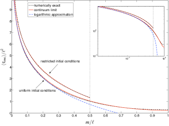
Figure 3: (Color online) Dependence of $\left\langle\tau_{\mathrm{enc}}\right\rangle/\ell^{2}$ as a function of $m/\ell$. Numerical results are shown with (black) dashed lines, the analytical continuum limits (6) with a (red) solid line, and the approximate expression (7) with a (blue) dash-dotted line. The inset shows the corresponding curves on a log–log plot. The mean first-encounter time relevant to epidemic propagation (walker $W_{1}$ uniform in its left overlap region, i.e., restricted initial conditions) is shown only for $m/\ell<\frac{1}{2}$, delimited by a vertical dotted line, since we consider only cases for which individuals always maintain an exclusive area.

Epidemic spread:-

To pass from microscopic interactions between walkers to macroscopic epidemic propagation, we consider a chain of habitats $H_{i}$, with $i=0$, $1$, …, each containing one confined walker, as sketched in Fig. 1. Starting with the left walker $0$ infected, the time to infect walker $n$ is $\tau^{(n)}$ = $\sum_{i=1}^{n}\tau_{i}$, where the $\tau_{i}$ are independent random variables giving the times for walker $i-1$ to infect walker $i$.

Each pair of walkers $i-1$ and $i$ is an identical copy of the same system (except the leftmost pair). However, the initial conditions are no longer uniform over the entire square, since when $W_{i-1}$ infects its neighbor $W_{i}$, the initial position of the latter must lie inside the corresponding overlap region $R_{i-1}$.

For the 2D walker, this corresponds to taking a distribution that is uniform only within two vertical strips, of width $m$ and height $2\ell$, at the left and right edges of the unfolded square domain shown in Fig. 2(b). By symmetry, the same result is obtained starting from two horizontal strips, so it can be approximated by a square strip of width $m$ around all edges of the domain, neglecting double counting in the corners where the horizontal and vertical strips overlap. In turn, we approximate this by the annulus $c\leq r\leq b$, where $c=2\ell(1-m/\ell)/\sqrt{\pi}$, with area equal to that of the square strip.

Taking uniform initial conditions in this annulus,with $\mathbb{P}_{\mathrm{in}}=0$ in Eq. (6), gives the MFET $\left\langle\tau_{\mathrm{enc}}\right\rangle=\left\langle\tau_{\mathrm{enc}}\right\rangle_{\mathrm{out}}$, whose expression is as in Eq. (5), but with $G_{n}(z,1)$ replaced by $G_{n}(z,v)$, with $v=m/[\sqrt{2}\ell(1-m/\ell)]$. This is compared to numerically-exact values in Fig. 3, with excellent agreement. We remark that the relevant regime for territorial animals is $m/\ell<1/2$, which corresponds to the presence of an exclusive core area.

If the infection is transmitted with probability $p<1$ at an encounter, then the walkers may meet repeatedly before the infection is transmitted, at any position in the overlap region. Returns to the target set, in which the 2D walker starts from one of the possible targets and comes back to hit any of them, must then be accounted for. The infection is transmitted at the $k$th encounter with probability $p_{k}:=p(1-p)^{k-1}$, giving the mean infection time $\left\langle\tau\right\rangle=\sum_{k=1}^{\infty}p_{k}\left\langle\tau|k\right\rangle,$ where $\left\langle\tau|k\right\rangle$ is the mean infection time conditional on infection occurring at the $k$th encounter. We have $\left\langle\tau|k\right\rangle=\left\langle\tau_{\mathrm{enc}}\right\rangle+(k-1)\left\langle\tau_{\mathrm{ret}}\right\rangle$, where $\left\langle\tau_{\mathrm{ret}}\right\rangle$ is the mean return time, giving

$$\left\langle\tau\right\rangle=\left\langle\tau_{\mathrm{enc}}\right\rangle+(\textstyle\frac{1}{p}-1)\left\langle\tau_{\mathrm{ret}}\right\rangle.$$ (8)

The mean return time $\left\langle\tau_{\mathrm{ret}}\right\rangle$ to a set $U$ can be calculated for discrete stochastic models, using the Kac recurrence lemma Kac (1947); Sanders (2009), as $\left\langle\tau_{\mathrm{ret}}\right\rangle=|\Omega|/|U|$, where $\Omega$ is the set of all possible configurations and $|\cdot|$ denotes the number of configurations in a set. Taking $U$ as the target set, we have $|U|=m$, giving $\left\langle\tau_{\mathrm{ret}}\right\rangle/\ell^{2}=1/m$, no longer a function of the dimensionless parameter $m/\ell$. Eq. (8) then gives the mean infection time $\left\langle\tau\right\rangle$ for any $p\leq 1$.

The previous results may now be combined to calculate the speed of propagation of an epidemic in the chain of habitats. We call $\omega(t)$ the position of the epidemic front, i.e., of the right-most infected walker Naether et al. (2008). The $n$th walker is infected at time $\tau^{(n)}$, at which time the front is at $\omega(\tau^{(n)})=n(\ell-m)$. Averaging over realizations, the front propagation is linear in $n$, with mean speed $(\ell-m)/\left\langle\tau\right\rangle$.

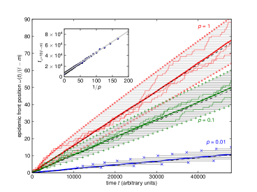
Figure 4: (Color online) Analytical (dashed lines) and numerical (thick lines, average over $100$ realizations) position $\omega(t)$ of the epidemic front for $\ell=20$ and $m=5$ and different transmission probabilities $p$, as a function of time $t$ (number of simulation steps); $\left\langle\tau_{\mathrm{enc}}\right\rangle\simeq 629$ for these values of $\ell$ and $m$. For illustrative purposes three realizations are shown for $p=1$ (red online) and $p=0.1$ (green). Crosses and gray horizontal bars show the range of possible times to arrive at a given front position, predicted by the law of the iterated logarithm. Inset: mean time to arrive at the front position $10(\ell-m)$ as a function of $1/p$, comparing analytical (solid line) and numerical results (dots; averaged over $200$ realizations).

Figure 4 compares the analytical result for the mean front position with numerical simulations, showing excellent agreement for different transmission probabilities $p$. Trajectories of individual realizations are also shown, as well as ranges of the possible times to arrive at a given front position, given by the law of the iterated logarithm Grimmett and Stirzaker (2001), which states that the infection time of walker $n$ lies within the interval $n\left\langle\tau\right\rangle\pm\sqrt{2n\ln(\ln n)}\,\sigma(\tau)$ for large enough $n$. Here, $\sigma(\tau)$ denotes the standard deviation of the first-encounter time, calculated analytically from the exact expression (3) for $F_{\mathrm{out}}$ for $p=1$, and numerically for the other values of $p$. This agrees with the several trajectories shown for $p=1$ and $p=0.1$, which are contained inside these bounds for large times.

For two-dimensional domains, this approach can be extended by looking for encounters along one axis, and conditioning on the walkers’ positions being identical also along the other axis. Preliminary results suggest different scalings as a function of domain size, depending on the form of the overlap region; this extension will form part of a future publication.

Our framework can also be extended to include spatial dependence of the transmission probability, due to heterogeneity in neighboring pairs, e.g., young versus adult individuals. The infection front then moves in a medium with infection rates which are not all equal (disordered); effective-medium theory Kenkre et al. (2009) provides the tools to calculate the propagation speed in terms of the transmission distribution.

The authors thank D. Boyer, N. Kenkre and H. Larralde for helpful discussions. Financial support from EPSRC grant EP/I013717/1 and DGAPA-UNAM PAPIIT grant IN116212 is acknowledged, and SP acknowledges a studentship from CONACYT, Mexico.

References

- Diekmann and Heesterbeek (2000) O. Diekmann and J. A. P. Heesterbeek, Mathematical Epidemiology of Infectious Diseases: Model Building, Analysis, and Interpretation (John Wiley and Sons, 2000).
- Belik et al. (2011) V. Belik, T. Geisel, and D. Brockmann, Phys. Rev. X 1, 1 (2011).
- Hufnagel et al. (2004) L. Hufnagel, D. Brockmann, and T. Geisel, Proc. Nat. Acad. Sci USA 101, 15124 (2004).
- Barrat et al. (2008) A. Barrat, M. Barthélemy, and A. Vespignani, Dynamical Processes on Complex Networks (Cambridge University Press, 2008).
- Ferguson et al. (2003) N. Ferguson, M. Keeling, W. J. Edmunds, R. Gani, B. Grenfell, R. Anderson, and S. Leach, Nature 425, 681 (2003).
- Colizza and Vespignani (2007) V. Colizza and A. Vespignani, Phys. Rev. Lett. 99, 148701 (2007).
- Aparicio and Pascual (2007) J. Aparicio and M. Pascual, Proc. Roy. Soc. B 274, 505 (2007).
- Aparicio and Vespigani (2011) J. Aparicio and A. Vespigani, Nature Physics 7, 581 (2011).
- Sanders and Larralde (2008) D. P. Sanders and H. Larralde, Europhys. Lett. 82, 40005 (2008).
- Sanders (2009) D. P. Sanders, Phys. Rev. E 80, 036119 (2009).
- Tejedor et al. (2011) V. Tejedor, M. Schad, O. Bénichou, R. Voituriez, and R. Metzler, J. Phys. A: Math. Theor. 44, 395005 (2011).
- Redner (2001) S. Redner, A Guide to First-Passage Processes (Cambridge University Press, 2001).
- Condamin et al. (2007) S. Condamin, O. Bénichou, and M. Moreau, Phys. Rev. E 75, 021111 (2007).
- Bénichou et al. (2010) O. Bénichou, C. Chevalier, J. Klafter, B. Meyer, and R. Voituriez, Nature Chemistry 2, 472 (2010).
- Meyer et al. (2011) B. Meyer, C. Chevalier, R. Voituriez, and O. Bénichou, Phys. Rev. E 83, 051116 (2011).
- Giuggioli et al. (2006) L. Giuggioli, G. Abramson, V. M. Kenkre, R. Parmenter, and T. L. Yates, J. Theor. Biol. 240, 126 (2006).
- Giuggioli et al. (2011) L. Giuggioli, J. R. Potts, and S. Harris, PLoS Comput. Biol. 7, 1002008 (2011).
- Ryals and Young (2012) B. Ryals and L.-S. Young, J. Stat. Phys. 146, 1089 (2012).
- Huveneers (2011) F. Huveneers, J. Stat. Phys. 146, 73 (2011).
- Chernov and Markarian (2006) N. Chernov and R. Markarian, Chaotic Billiards, Mathematical Surveys and Monographs, 127 (American Mathematical Society, Providence, RI, 2006).
- Crank (1975) J. Crank, The Mathematics of Diffusion (Oxford University Press, 1975).
- Kac (1947) M. Kac, Bull. Amer. Math. Soc. 53, 1002 (1947).
- Naether et al. (2008) U. Naether, E. Postnikov, and I. Sokolov, Eur. Phys. J. B 65, 353 (2008).
- Grimmett and Stirzaker (2001) G. Grimmett and D. Stirzaker, Probability and Random Processes (Oxford University Press, 2001), 3rd ed.
- Kenkre et al. (2009) V. Kenkre, Z. Kalay, and P. Parris, Phys. Rev. E 79, 011114 (2009).