Magnetic field induced localization in 2D topological insulators

Abstract

Localization of the helical edge states in quantum spin Hall insulators requires breaking time reversal invariance. In experiments this is naturally implemented by applying a weak magnetic field $B$. We propse a model based on scattering theory that describes the localization of helical edge states due to coupling to random magnetic fluxes. We find that the localization length is proportional to $B^{-2}$ when $B$ is small, and saturates to a constant when $B$ is sufficiently large. We estimate especially the localization length for the HgTe/CdTe quantum wells with known experimental parameters.

The prediction and discovery of quantum spin Hall insulators (QSHIs) Kane and Mele (2005a, b); Bernevig et al. (2006); Konig et al. (2007) has opened a door to an unexpected category of topological phases in condensed matter Kitaev (2009); Schnyder et al. (2009); Hasan and Kane (2010); Qi and Zhang (2011), and revealed a new route to investigations of edge/boundary-state physics Roth et al. (2009); Büttiker (2009); C.Brüne et al. (2012). Although the prototypes of QSHIs Kane and Mele (2005a); Bernevig et al. (2006) are mainly based on two copies of quantum Hall insulators, which have been investigated for more than three decades von Klitzing et al. (1980); Haldane (1988), it was soon realized that the fundamental importance of time reversal invariance (TRI) distinguishes the two systems in a profound way Kane and Mele (2005b). Indeed, QSHIs, unlike the $\mathbb{Z}$-classified quantum Hall insulators Thouless et al. (1982), belong to a class of two-dimensional time-reversal-invariant $\mathbb{Z}_{2}$ topological insulators Kane and Mele (2005b). The defining feature of QSHIs, as its name suggests, is a pair of helical edge states that persist in the bulk insulating gap of the system Kane and Mele (2005a, b); Bernevig et al. (2006); Konig et al. (2007); Roth et al. (2009).

The topological power of QSHIs lies precisely in the robustness of the helical edge states against generic perturbations due to unavoidable disorder in every experimental setup, unless TRI is broken. In the presence of both TRI breaking and disorder, the helical edge states will be localized, and the general framework of Anderson’s localization theory applies Anderson (1958). Nevertheless, the localization of the helical edge states distinguishes itself from conventional one-dimensional localization when the focus is placed on the crucial role TRI plays in the problem. This point becomes especially relevant as TRI can be broken continuously, for instance, by turning on a magnetic field gradually. Indeed, the sensibility of transport though helical edge states to weak magnetic field has been demonstrated experimentally in the measurement of magneto-conductance in topologically nontrivial HgTe/CdTe quantum wells Konig et al. (2007, 2008). Related theoretical analyses have been carried out that include the interplay between TRI-breaking and disorder, but mainly consider magnetic impurities Tanaka et al. (2011); Hattori (2011), or bulk random potential combined with magnetic field J. Maciejko and Zhang (2010). A transparent edge theory that focuses on the magnetic-field-dependent localization of the helical edge states, however, is still missing.

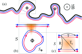
Figure 1: (a) Helical edge states in a disordered QSHI in a uniform magnetic field. Occasional occurrences of constrictions along the edge lead to Fabry-Perot-type loops where Aharonov-Bohm phases due to magnetic fluxes can accumulate. (b) The scattering of the helical edges by one of these loops, described by a scattering matrix ${\cal S}$, can be divided into two parts: the scattering between two pairs of helical edge states ($S$), and the propagation of one of these pairs around the loop ($S_{\Phi}$). (c) Three types of scattering probabilities, $T$, $R$ and $T_{s}$, that are relevant to the scattering between two pairs of helical edge states.

In this paper we propose a model that explicitly addresses the question on how the localization of helical edge states occurs as a weak magnetic field is gradually turned on. Our model is based on the scattering theory of edge states in the presence of generic edge disorder. In particular we consider the existence of alternative paths for the edge states due to, e.g., constrictions formed at the rough edges of realistic samples (see Fig. 1), which further allows for loops of the helical edge states. The magnetic field penetrating though these loops results in broken TRI that is experienced by the helical edge states in the form of finite random fluxes. We show that these random fluxes necessarily lead to localization of the helical edge states with universal behaviors in two regimes: immediately after the magnetic field is turned on, the localization length becomes finite and decreases as $B^{-2}$; when the standard deviation of the random fluxes (proportional to $B$) is comparable to or larger than one magnetic flux quantum, the localization length saturates to a constant. In-between these two regimes, damped oscillations of the localization length may arise depending on the distribution of the random fluxes. Our results provide a clear illustration of the symmetry-breaking-induced localization in QSHIs.

We start to introduce our model by considering one of its possible realizations, depicted in Fig. 1. The edge roughness of a realistic QSHI sample may lead to occasional constrictions (at one edge) where the helical edge states can either tunnel across or pass around. As a consequence, loops can form and attach to the propagating path of the helical edge states. When a perpendicular magnetic field is applied to the sample , each of these loops acts as a magnetic flux impurity, to be distinguished from usual magnetic impurities. Individually such an impurity works like a Fabry-Perot scatterer (see Fig. 1b), where the scattering probability amplitudes depend on the Aharonov-Bohm (AB) phase, owing to the magnetic flux, acquired by electrons circling around the loop. The collective action of a random distribution of these scatterers causes localization of the helical edge states with an explicit dependence on the magnetic field. The main part of this problem can be tackled consistently by scattering theory, as we now show.

To analyze the scattering of the helical edge states by a single magnetic flux impurity (see Fig. 1), we divide the full scattering process into two effective parts: the local scattering between two pairs of helical states, and the free propagation of one pair of helical states that closes the loops. For simplicity, we assume that the first part does not depend on magnetic field, hence respects local TRI, while the second part contains the entire information about the magnetic flux by means of AB phases that enter the propagators.

Owing to the local TRI, the scattering between two pairs of helical states, described by a $4\times 4$ scattering matrix $S$, has the following constraint:

$$S=\Theta\ S^{\dagger}\ \Theta^{-1},$$ (1)

where ${\Theta}$ is the time-reversal operator. We choose a specific basis ordered as $(R_{1},L_{1},L_{2},R_{2})$, where $R_{i}$ ($L_{i}$) stands for the right (left) mover of the $i$-th Kramers pair ($i=1,2$), such that the time-reversal operator reads

$$\Theta=\begin{pmatrix}-i\sigma_{y}\kappa&0\\ 0&-i\sigma_{y}\kappa\\ \end{pmatrix}$$ (2)

with $\sigma_{y}$ the Pauli matrix and $\kappa$ the complex-conjugate operator. Consequently, the scattering matrix $S$ satisfying Eq. (1) necessarily has the following form:

$$S=\left(\begin{array}[]{cccc}t_{1}&0&r^{\prime}&s^{\prime}\\ 0&t_{1}&-s&r\\ r&-s^{\prime}&t_{2}&0\\ s&r^{\prime}&0&t_{2}\end{array}\right)\,.$$ (3)

Here $t_{i}$ stands for the direct transmission for Kramers pair $i$; $r$ ($r^{\prime}$) stands for the reflection from a right (left) mover to a left (right) mover; $s$ and $s^{\prime}$ represent the transmission by switching to another Kramers pair. Importantly, zeros in $S$ signify the absence of direct back-scattering within one Kramers pair due to TRI. Taking into account the unitarity of the scattering matrix, the parametrization of $S$ can be further simplified as (up to an unimportant global phase factor): $t_{1}=-t_{2}^{*}=t$, $r^{\prime}=r^{*}$, $s^{\prime}=s^{*}$, and $T+R+T_{s}=1$, where $T=|t|^{2}$, $R=|r|^{2}$ and $T_{s}=|s|^{2}$.

The free propagation of Kramers pair 2 leads to a $2\times 2$ scattering matrix $S_{\Phi}$ that is diagonal in the basis $(L_{2},R_{2})$, given by

$$S_{\Phi}=\left(\begin{array}[]{cc}e^{i(\varphi+\phi)}&0\\ 0&e^{i(\varphi-\phi)}\end{array}\right)$$ (4)

with $\varphi$ the dynamical phase and $\phi$ the AB phase (equal to the total flux enclosed by the loop in units of $h/2\pi e$).

Combining the two parts above, we find the final scattering matrix ${\cal S}$ for Kramers pair 1, in the basis $(R_{1},L_{1})$, to be

$${\cal S}=\begin{pmatrix}|t|+RZ_{+}+T_{s}Z_{-}&-(rs)^{*}\Delta Z\\ -rs\Delta Z&|t|+RZ_{-}+T_{s}Z_{+}\\ \end{pmatrix},$$ (5)

$$\text{where}\qquad Z_{\pm}=\frac{e^{i(\varphi\pm\phi)}}{1+|t|e^{i(\varphi\pm\phi)}}\,,$$ (6)

$$\Delta Z=Z_{+}-Z_{-}=\frac{i}{|t|}\,\frac{\sin\phi}{\cos\phi+\cosh(\ln|t|+i\varphi)}\,,$$ (7)

and the phase of $t^{*}$ has been absorbed into the dynamical phase $\varphi$. The back-scattering probability can be obtained immediately:

$${\cal R}=\frac{RT_{s}}{T}\,\frac{\sin^{2}\phi}{\bigl{|}\cos\phi+\cosh(\ln|t|+i\varphi)\bigr{|}^{2}}\,.$$ (8)

Evidently, for the helical edge states to be back-scattered with finite probability, two conditions must be fulfilled. First, it is necessary that both $R$ and $T_{s}$ are finite. If one of these two tunneling probabilities is zero, the system essentially reduces to two decoupled copies of quantum Hall edge states, and back-scattering is known to be prohibited for either copy Büttiker (1988). Only when both tunneling processes ($R$ and $T_{s}$) are allowed, the system belongs truly to the $\mathbb{Z}_{2}$-classified symmetry class where TRI plays a central role. It follows that the second necessary condition for back-scattering to occur is to break the global TRI by having $\phi\neq 0\mod\pi$. The cooperation of these two conditions clearly illustrates the underlying protection mechanism, from the scattering point of view, for the helical edge states of QSHIs.

At disordered sample edges, the magnetic flux impurities will occur randomly, and the helical edge states will eventually be localized as a consequence of finite back-scattering probabilities for individual scatterers. Here, we assume not only that the variables (including phases and scattering amplitudes) for each individual scatterer are random, but also that different scatterers are completely independent such that the relative scattering phases for two consecutive scatterers are uniformly distributed. The localization length of the helical edge states in this scenario can be extracted from the appropriate scaling variable $\ln{\cal T}$, where ${\cal T}=1-{\cal R}$ is the total transmission probability for the effective one-dimensional system Anderson et al. (1980).

The total transmission probability ${\cal T}_{N}$ through $N$ scatterers can be calculated by multiplying the transfer matrices that relate the scattering amplitudes on the right side of each individual scatterer (labeled $i$, $i=1,...,N$) to those on the left. A general transfer matrix reads

$$M_{i}=\frac{1}{\tau_{i}}\,\left(\begin{array}[]{cc}\lambda_{i}&\rho_{i}\\ \rho^{*}_{i}&\lambda^{*}_{i}\end{array}\right),$$ (9)

where $\tau_{i}$ corresponds to the transmission amplitudes (diagonal entries in ${\cal S}$) for the $i$-th scatterer, $\rho_{i}$ corresponds to the reflection amplitudes (off-diagonal entries in ${\cal S}$), and $\lambda_{i}$ is a phase factor that is independent for each scatterer. Note that the dynamical phase for the free propagation of the helical states in-between two consecutive scatterers ($i$ and $i+1$, say) can be obviously incorporated into the above transfer matrix while preserving its general form. Note also that multiplications of the transfer matrices preserve the general form as well. We will put an overhead tilde to distinguish the amplitudes involving $i$ consecutive scatterers from those involving only a single ($i$-th) scatterer. Then ${\cal T}_{N}$ is given by

$${\cal T}_{N}=|\tilde{\tau}_{N}|^{2}=\frac{|\tilde{\tau}_{N-1}|^{2}|\tau_{N}|^{2}}{\bigl{|}1+|\tilde{\rho}_{N-1}\rho_{N}|e^{i\theta}\bigr{|}^{2}},$$ (10)

with $e^{i\theta}=\tilde{\lambda}_{N-1}\lambda_{N}\tilde{\rho}_{N-1}\rho_{N}^{*}/|\tilde{\rho}_{N-1}\rho_{N}|$. Our assumption of independent scatterers implies that $\theta$ is uniformly distributed in $[0,2\pi)$. It follows that the mean of the scaling variable $\langle\ln{\cal T}\rangle$ becomes simply additive Anderson et al. (1980)

$$\langle\ln{\cal T}_{N}\rangle=\langle\ln{\cal T}_{N-1}\rangle+\langle\ln|\tau_{N}|^{2}\rangle,$$ (11)

where $\langle\ln\bigl{|}1+|\tilde{\rho}_{N-1}\rho_{N}|e^{i\theta}\bigr{|}^{2}\rangle$ has vanished after averaging over $\theta$.

The inverse localization length $\gamma=1/\ell_{\text{loc}}$ is defined in terms of the scaling variable as: Anderson et al. (1980); Pendry (1994); Müller and Delande (2011)

$$\gamma=-\lim_{N\rightarrow\infty}\frac{n}{N}\left\langle\ln{\cal T}_{N}\right\rangle=-n{\langle\ln(1-{\cal R})\rangle},$$ (12)

where $n$ is the linear density of the scatterers. The final average $\langle\ln(1-{\cal R})\rangle$ is over certain distributions of independent variables including $\varphi$, $\phi$ and scattering amplitudes that appear in Eq. (8) for a single scatterer. We are interested in the weak back-scattering case for each individual scatterer (${\cal R}\ll 1$), thus

$$\gamma\simeq n{\langle{\cal R}\rangle}.$$ (13)

The average in terms of the arbitrary dynamical phase $\varphi$ can be carried out exactly, and yields

$$\gamma=n\left\langle\frac{RT_{s}}{R+T_{s}}\,\frac{1+T}{T}\,\frac{\sin^{2}\phi}{\sin^{2}\phi+\frac{(1-T)^{2}}{4T}}\right\rangle.$$ (14)

By further using the fact that $\phi=BA(2\pi e/h)$, where the magnetic field $B$ is taken to be uniform and $A$ is the area enclosed by the helical loops, we will only need to average over distributions of the scattering amplitudes and the area $A$ in order to estimate the localization length $\ell_{\text{loc}}=1/\gamma$. One immediate consequence of Eq. (14) is that the localization length is magnetic field symmetric, which is certainly expected.

An important regime that we are particularly interested in is the weak magnetic field regime, where $B\bar{A}\ll h/e$ with $\bar{A}$ the mean of $A$. In this regime Eq. (14) becomes (assuming $T$ is not too close to $1$)

$$\gamma=\alpha B^{2}$$ (15)

$$\text{with}\qquad\alpha=4n\Bigl{(}\frac{2\pi e}{h}\Bigr{)}^{2}\Bigl{\langle}\frac{RT_{s}}{(R+T_{s})^{3}}(1+T)\Bigr{\rangle}\langle A^{2}\rangle\,.$$ (16)

Manifestly $\alpha$ is a constant factor for given distributions of scattering amplitudes and $A$. The $B^{2}$-dependence of the inverse localization length here is a universal result of our model in the sense that it does not depend on the specific distributions of variables for individual scatterers. It implies that the localization length of the helical edge states is finite at weak magnetic field and diverges only as $1/B^{2}$ when the magnetic field is vanishing. Furthermore, the low-temperature magneto-conductance of a QSHI should also vary as $B^{2}$ in the weak magnetic field limit, that is, $\delta G(B)=G(0)-G(B)\propto B^{2}$. This contrasts our result with the linear magneto-conductance behavior previously found on a lattice model with bulk impurity potentials J. Maciejko and Zhang (2010).

Another interesting regime is when the magnetic field is strong enough such that both $B\bar{A}$ and $B\sigma_{A}$ (with $\sigma_{A}\equiv\sqrt{\langle(A-\bar{A})^{2}\rangle}$ being the standard deviation) are comparable or larger than a flux quantum $h/e$. In this regime we can approximate the average in terms of $A$ as an average over a uniform distribution of $\phi$, which yields

$$\gamma_{\text{sat}}=2n\left\langle\frac{RT_{s}}{R+T_{s}}\right\rangle\,.$$ (17)

This especially simple result again shows a universal behavior in our model–the inverse localization length saturates at relatively strong magnetic field irrespective of the specific distributions of scattering variables. However the actual value of $\gamma_{\text{sat}}$ certainly depends on the distributions of $R$ and $T_{s}$. Moreover, the above formula re-emphasizes the importance of allowing both tunneling processes represented by $R$ and $T_{s}$ to evoke a true protection mechanism due to TRI.

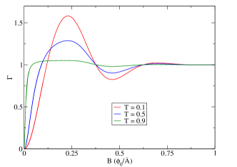
Figure 2: $\Gamma(B)$ for different values of $T$, where $A$ is assumed to take a normal distribution with $\sigma_{A}/\bar{A}=0.3$.

In-between the two regimes discussed above, we need to consider the specific distributions of the variables in Eq. (14). Let us first focus on the behavior of $\gamma$ by assuming that $A$ has a Gaussian distribution characterized by the mean $\bar{A}$ and the standard deviation $\sigma_{A}$. It is instructive in this case to look at the function $\Gamma(B)\equiv[(1+T)/2T]\left\langle\sin^{2}\phi/[\sin^{2}\phi+(1-T)^{2}/4T]\right\rangle_{A}$ with the average only taken in terms of $A$. $\Gamma(B)$ has been defined such that it saturates to the value $1$ at sufficiently strong magnetic field. In Fig. 2 we plot the numerically obtained $\Gamma(B)$ for various $T$ and fixed $\bar{A}$ and $\sigma_{A}$. Right after the magnetic field is turned on, $\Gamma(B)$ shows a quadratic increase irrespective of the assumed $T$ or the distribution of $A$. Before $\Gamma(B)$ saturates, it undergoes damped oscillations when $\sigma_{A}/\bar{A}$ is small. These oscillations are due to the collective AB effect for the helical loops in our model: the loops enclosing similar area lead to AB oscillations of similar period; they contribute coherently to the back-scattering of the helical edge states; the magnetic field dependence of the total transmission is thus shaped by the AB effect at individual scatterers when $B\sigma_{A}$ is significantly smaller than $\phi_{0}=h/e$. The period of the oscillations is roughly $\phi_{0}/2\bar{A}$, where the factor $1/2$ is obviously a consequence of $\Gamma$ (and hence $\gamma$) only depending on $\sin^{2}\phi$. The overall amplitude of the oscillations is suppressed for large $T$ and enhanced for small $T$. The reason is intuitively clear: the more the helical edge states are scattered into the loops, the more pronounced the resulting AB effect.

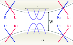
Figure 3: A schematic view of a constriction where two pairs of helical edge states (indicated by the linear bands) are coupled (indicated by the mixed bands) in a region of length $L$ and separation $W$.

Now we address the issue of the scattering amplitudes which have only been assumed to be phenomenological parameters in the scattering matrix $S$ so far. To this end we investigate a constriction depicted in Fig. 3, which is described by the following effective Hamiltonian:

$${\cal H}=\begin{pmatrix}\hbar v_{F}\hat{k}_{x}&0&m(x)&\delta(x)\\ 0&-\hbar v_{F}\hat{k}_{x}&-\delta(x)&m(x)\\ m(x)&-\delta(x)&-\hbar v_{F}\hat{k}_{x}&0\\ \delta(x)&m(x)&0&\hbar v_{F}\hat{k}_{x}\\ \end{pmatrix},$$ (18)

where $v_{F}$ is the Fermi velocity for the helical edge states, $m(x)$ and $\delta(x)$ represent $x$-dependent coupling between the edge states, and the basis is ordered as $(R_{1},L_{1},L_{2},R_{2})$. The above Hamiltonian manifestly respects TRI: ${\cal H}=\Theta{\cal H}\Theta^{-1}$. This Hamiltonian can be derived from microscopic models such as the Bernevig-Hughes-Zhang (BHZ) model for HgTe/CgTe quantum wells Bernevig et al. (2006); Konig et al. (2007, 2008); Zhou et al. (2008); Krueckl and Richter (2011). For simplicity we take $m(x)=m_{W}\theta(x)\theta(L-x)$ and $\delta(x)=\delta_{W}\theta(x)\theta(L-x)$ with $\theta(x)$ the Heaviside step function and $m_{W}$ and $\delta_{W}$ two constants determined by the constriction separation $W$. In the case of HgTe/CgTe quantum wells, a nonvanishing $\delta$ term owes its existence to the presence of bulk-inversion asymmetry Konig et al. (2007, 2008).

The scattering amplitudes for this constriction, corresponding to $S$ in Eq. (3), can be easily derived (see supplementary materials):

$$t =i\cos(\delta_{W}L/\hbar v_{F})/\zeta,$$ (19)

$$s =\sin(\delta_{W}L/\hbar v_{F})/\zeta,$$ (20)

$$r =m_{W}\sin(qL)/\hbar v_{F}q\zeta,$$ (21)

where $q=\sqrt{E^{2}-m_{W}^{2}}/\hbar v_{F}$ can be either real or imaginary depending on the energy $E$, and $\zeta=|(E/\hbar v_{F}q)\sin(qL)+i\cos(qL)|$ is a normalization factor. Clearly $r$ vanishes when $m_{W}=0$, which shows the fact that $m$ couples $R_{1}$ ($L_{1}$) to $L_{2}$ ($R_{2}$); $s$ vanishes when $\delta_{W}=0$, which shows the fact that $\delta$ couples $R_{1}$ ($L_{1}$) to $R_{2}$ ($L_{2}$). For low energy ($|E|<m_{W}$) scattering states, $R/(T+T_{s})\simeq\sinh^{2}(m_{W}L/\hbar v_{F})$ if $|E|\ll m_{W}$, and $R/(T+T_{s})\simeq(m_{W}L/\hbar v_{F})^{2}$ if $|E|\simeq m_{W}$, meaning that the reflection dominates as long as $L$ is large compared with $\hbar v_{F}/m_{W}$. In this regime, Eq. (12) reduces to $\gamma\simeq 4n\langle T_{s}\rangle\langle\sin^{2}\phi\rangle$.

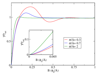
Figure 4: Inverse localization length $\gamma$ as a function of magnetic field $B$, for different distributions of loop area $A$. It shows a $B^{2}$-increase in the weak $B$ limit (inset) and a saturation at relatively high field. In-between, damped oscillations may occur if $\sigma_{A}/\bar{A}<1$. The saturation value $\gamma_{\text{sat}}$ is sample-dependent but has an order of magnitude $0.01n$ (with $n$ the linear density of the scatterers) in our realistic estimations.

More generally the average with respect to the scattering amplitudes has to be performed numerically by taking certain distributions of $W$ and $L$ (at a certain energy $E$). The advantage of this change of variables is that $W$ and $L$, unlike the scattering amplitudes, are in principle independent to each other. In total, this leads to three independent geometric variables, $W$, $L$ and $A$, that remain to be averaged on in our final evaluation of $\gamma$ as a function of magnetic field $B$ (we will not make any assumption on the density $n$ of scatterers and leave it as a parameter). After carrying out these averages numerically (see supplementary materials for details), we show the typical results in Fig. 4. The qualitative behavior of $\gamma(B)$ in Fig. 4 is essentially the same as that of $\Gamma(B)$ in Fig. 2, except that $\gamma(B)$ is shown for various ratios $\sigma_{A}/\bar{A}$ whereas the scattering amplitudes have been averaged out. The universal features which we can observe are that $\gamma$ increases as $B^{2}$ at weak magnetic field and saturates at sufficiently strong magnetic field. Despite the fact that the exact value of $\gamma_{\text{sat}}$ depends on the energy $E$ and the distributions of $W$ and $L$, the order of magnitude of $\gamma_{\text{sat}}$ turns out to be consistently $0.01n$ for all cases with realistic considerations (see supplementary materials). We also observe in the intermediate regime damped oscillations of $\gamma$ which are pronounced if $\sigma_{A}/\bar{A}$ is small but suppressed as long as $\sigma_{A}/\bar{A}$ is close to or larger than $1$. We point out here that $\gamma(B)$ has a local minimum/maximum, hence the localization length has a local maximum/minimum, whenever $B$ is roughly an integer/half-integer multiple of $\phi_{0}/2\bar{A}$ – this is where the TRI is maximally preserved/broken.

To summarize, we have investigated a simple yet illuminating model that demonstrates a magnetic-field-dependent localization of the helical edge states in quantum spin Hall insulators. We have identified universal, sample-independent features, as well as an interesting but sample-specific feature in this model. With known parameters for the HgTe/CgTe quantum wells, we have also estimated quantitatively the localization length. Both the qualitative and the quantitative results can be examined by experiments.

I Supplementary material

II Derivation of Eqs. (19-21)

In this section we derive the scattering amplitudes, given by Eqs. (19-21) in the main text, for the constriction described by the Hamiltonian (18) in the main text. By assuming $m(x)=m_{W}\theta(x)\theta(L-x)$ and $\delta(x)=\delta_{W}\theta(x)\theta(L-x)$ with $\theta(x)$ the Heaviside step function and $m_{W}$ and $\delta_{W}$ two constants, we divide the constriction into three regions: $x<0$, $0\leq x\leq L$ and $x>L$. The scattering amplitudes are obtained by matching energy eigenstate wavefunctions for adjacent regions.

The energy eigenstates in the regions $x<0$ and $x>L$ are trivial:

$$\Psi_{a}(x<0)=\begin{pmatrix}a_{1}e^{ik_{0}x}\\ a_{2}e^{-ik_{0}x}\\ a_{3}e^{-ik_{0}x}\\ a_{4}e^{ik_{0}x}\\ \end{pmatrix},\qquad\Psi_{c}(x>L)=\begin{pmatrix}c_{1}e^{ik_{0}x}\\ c_{2}e^{-ik_{0}x}\\ c_{3}e^{-ik_{0}x}\\ c_{4}e^{ik_{0}x}\\ \end{pmatrix},$$ (22)

where $k_{0}=E/\hbar v_{F}$. In the region $0\leq x\leq L$, the energy eigenstate is given by

$$\Psi_{b}(x)=b_{1}\left(\begin{array}[]{c}1\\ -e^{-i\theta}\\ e^{-i\theta}\\ -1\end{array}\right)e^{ik_{1}x}+b_{2}\left(\begin{array}[]{c}1\\ e^{i\theta}\\ e^{i\theta}\\ 1\end{array}\right)e^{ik_{2}x}+b_{3}\left(\begin{array}[]{c}1\\ e^{-i\theta}\\ e^{-i\theta}\\ 1\end{array}\right)e^{ik_{3}x}+b_{4}\left(\begin{array}[]{c}1\\ -e^{i\theta}\\ e^{i\theta}\\ -1\end{array}\right)e^{ik_{4}x},$$ (23)

where $\theta=\arccos(E/m_{W})$, $k_{1}=-k_{2}=\delta_{W}/\hbar v_{F}+q$ and $k_{3}=-k_{4}=-\delta_{W}/\hbar v_{F}+q$ with $q=\sqrt{E^{2}-m_{W}^{2}}/\hbar v_{F}=i(m_{W}/\hbar v_{F})\sin\theta$. Note that both $\theta$ and $q$ can be complex depending on the energy $E$. Note also that the basis for the above wavefunctions is ordered as $(R_{1},L_{1},L_{2},R_{2})$ (see Fig. 3 of the main text).

To start with we assume that the only incoming state is from channel $R_{1}$, that is, $a_{1}=1$ and $a_{4}=c_{2}=c_{3}=0$. Then we need to match the wavefunctions such that

$$\Psi_{b}(x=0)=\Psi_{a}(x=0)=\begin{pmatrix}1\\ a_{2}\\ a_{3}\\ 0\\ \end{pmatrix},$$ (24)

$$\Psi_{b}(x=L)=\Psi_{c}(x=L)=\begin{pmatrix}c_{1}\\ 0\\ 0\\ c_{4}\\ \end{pmatrix}e^{ik_{0}L}\,.$$ (25)

The above equations fix the values of $b_{i}$ $(i=1,2,3,4)$, and hence the values of $a_{2}$, $a_{3}$, $c_{1}$ and $c_{4}$. In particular, $a_{2}$ can be identified as the backscattering amplitude and we find $a_{2}=0$ identically; $a_{3}$ can be identified as $r$; $c_{1}$ can be identified as $t$; $c_{4}$ can be identified as $s$. We find:

$$t =i\cos(\delta_{W}L/\hbar v_{F})\sin\theta/\sin(qL-\theta),$$ (26)

$$s =\sin(\delta_{W}L/\hbar v_{F})\sin\theta/\sin(qL-\theta),$$ (27)

$$r =-i\sin(qL)/\sin(qL-\theta),$$ (28)

which are precisely Eqs. (19-21) in the main text after removing an unimportant common phase factor. By assuming differently the incoming states, we can construct the full scattering matrix for the constriction. Both the unitarity of the scattering matrix and the symmetry relations between the matrix elements can be easily checked.

III Numerical simulations to extract the distributions of scattering probabilities

In this section we extract from numerical simulations the distributions of the scattering probabilities for the constriction illustrated in Fig. 3 of the main text. In our simulations we employ a six-terminal setup as shown in Fig. 5. This setup is equivalent to a Hall-bar setup. We define a point contact with cosine profiles to simulate the effect of the constriction. The point contact has two parameters: its length $L$ and its separation $W$. The depleted regions are defined by a sufficiently high on-site potential (compared with the band width).

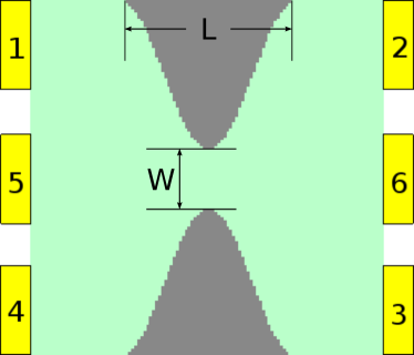
Figure 5: Schematic setup for the simulations.

The model Hamiltonian for the central region of the setup is the tight-binding Hamiltonian corresponding to the Bernevig-Hughes-Zhang (BHZ) model Bernevig et al. (2006):

$$H_{BHZ}(\vec{k})=\begin{pmatrix}h(\vec{k})&-i\Delta\sigma_{y}\\ i\Delta\sigma_{y}&h^{*}(-\vec{k})\\ \end{pmatrix}$$ (29)

with $$h(\vec{k})=(C-Dk^{2})+Ak_{x}\sigma_{x}-Ak_{y}\sigma_{y}+(M-Bk^{2})\sigma_{z}$$ (30)

and $\sigma_{i}$ ($i=x,y,z$) are Pauli matrices. The block-off-diagonal term, proportional to $\Delta$, is a spin-orbit interaction term due to the bulk inversion asymmetry in HgTe/CdTe quantum wells Konig et al. (2007, 2008). We list in Table 1 the experimentally obtained parameters for the above Hamiltonian, as well as the lattice spacing $a$ adopted to discretize this Hamiltonian. We will measure length in units of $a$ hereafter. With these parameters we estimate the Fermi velocity for the helical edge states to be $v_{F}\simeq 3.8\times 10^{5}$ m/s.

$A$ (meV$\cdot$nm)	$B$ (meV$\cdot$nm2)	$C$ (meV)	$D$ (meV$\cdot$nm2)	$M$ (meV)	$\Delta$ (meV)	$a$ (nm)
364.5	-686	-7.5	-512	-10	1.6	5

Table 1: Parameters for the simulations. Note that the parameter $C$, which corresponds to an overall constant energy shift, takes the value so that the edge bands cross at $E=0$.

The scattering probabilities for the constriction that are needed in the main paper can be identified in the current setup as follows:

$$T=T_{21},\;T_{s}=T_{31},\;R=T_{41},$$ (31)

where $T_{ji}$ is the transmission probability from contact $i$ to contact $j$. These transmission probabilities can be calculated by using the standard Green’s function technique Fisher and Lee (1981). We also check the sum rule $T_{sum}=T_{21}+T_{31}+T_{41}=1$ to ensure the validity of our results.

For the distributions of the scattering probabilities we need to assume reasonable distributions for $L$ and $W$. Without sufficient knowledge from experiments we make the following assumptions: $L$ is uniformly distributed in the range $(0,2l_{SO})$ with the spin-orbit length $l_{SO}=\hbar v_{F}/\Delta\simeq 30a$; $W$ is uniformly distributed in the range $(0,2\xi)$ with $\xi$ the penetration depth of the edge states. $\xi$ is energy dependent and its order of magnitude is given by $\hbar v_{F}/M\simeq 5a$. We will fix the energy at $E=0.5$ meV for the results presented below, where $\xi\simeq 10a$. We have checked the robustness of our results with other values of energy and/or other reasonable distributions (e.g. Gaussian distribution) of $L$ and $W$.

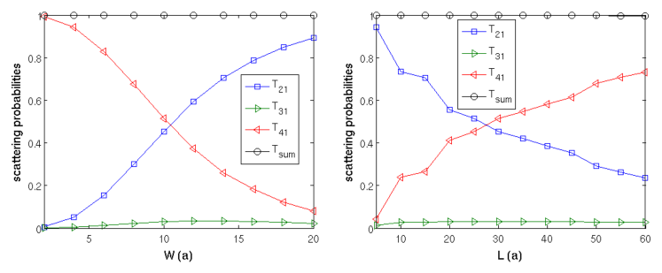
Figure 6: Typical dependences of scattering probabilities on $W$ and $L$. For the left panel, $L=30a$; for the right panel, $W=10a$.

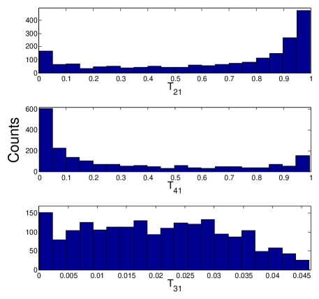
Figure 7: Histograms showing the distributions of the scattering probabilities.

As results of our simulation, we show the typical dependences of the scattering probabilities on $L$ and $W$ in Fig. 6, and the histograms for the distributions of the scattering probabilities in Fig. 7. To obtain our final result presented in Fig. 4 of the main text, we simply generate samples with randomly chosen $L$ and $W$ according to our assumptions; no accurate distribution functions for the scattering probabilities are actually needed for our purpose.

References

- Bernevig et al. (2006) B. A. Bernevig, T. A. Hughes, and S.-C. Zhang, Science 314, 1757 (2006).
- Konig et al. (2007) M. Konig, S. Wiedmann, C. Brune, A. Roth, H. Buhmann, L. W. Molenkamp, X.-L. Qi, and S.-C. Zhang, Science 318, 766 (2007).
- Konig et al. (2008) M. Konig, H. Buhmann, L. W. Molenkamp, T. Hughes, C.-X. Liu, X.-L. Qi, and S.-C. Zhang, J. Phys. Soc. Jpn 77, 031007 (2008).
- Fisher and Lee (1981) D. S. Fisher and P. A. Lee, Phys. Rev. B 23, 6851 (1981).