Sequential multi-sensor change-point detection

Abstract

We develop a mixture procedure to monitor parallel streams of data for a change-point that affects only a subset of them, without assuming a spatial structure relating the data streams to one another. Observations are assumed initially to be independent standard normal random variables. After a change-point the observations in a subset of the streams of data have nonzero mean values. The subset and the post-change means are unknown. The procedure we study uses stream specific generalized likelihood ratio statistics, which are combined to form an overall detection statistic in a mixture model that hypothesizes an assumed fraction $p_{0}$ of affected data streams. An analytic expression is obtained for the average run length (ARL) when there is no change and is shown by simulations to be very accurate. Similarly, an approximation for the expected detection delay (EDD) after a change-point is also obtained. Numerical examples are given to compare the suggested procedure to other procedures for unstructured problems and in one case where the problem is assumed to have a well-defined geometric structure. Finally we discuss sensitivity of the procedure to the assumed value of $p_{0}$ and suggest a generalization.

abstractwidth290pt

T1Supported in part by NSF Grant 1043204 and Stanford General Yao-Wu Wang Graduate Fellowship.

and

1 Introduction

Single sequence problems of change-point detection have a long history in industrial quality control, where an observed process is assumed initially to be in control and at a change-point becomes out of control. It is desired to detect the change-point with as little delay as possible, subject to the constraint that false detections occurring before the true change-point are very rare. Outstanding early contributions are due to Page Page1954 , Page1955 , Shiryaev Shiryaev1963 and Lorden Lorden1971 .

We assume there are parallel streams of data subject to change-points. More precisely suppose that for each $n=1,\ldots,N$, we make observations $y_{n,t}$, $t=1,2,\ldots.$ The observations are mutually independent within and across data streams. At a certain time $\kappa$, there are changes in the distributions of observations made at a subset $\mathcal{N}\subset\{1,\ldots,N\}$ of cardinality $|\mathcal{N}|\leq N$. Also denote by $\mathcal{N}^{c}$ the set of unaffected data streams. The change-point $\kappa$, the subset $\mathcal{N}$ and its size, and the size of the changes are all unknown. As in the case of a single sequence, $N=1$, the goal is to detect the change-point as soon as possible after it occurs, while keeping the frequency of false alarms as low as possible. In the change-point detection literature, a surrogate for the frequency of false alarms is the average-run-length (ARL), defined to be the expected time before incorrectly announcing a change of distribution when none has occurred.

It may be convenient to imagine that the data streams represent observations at a collection of $N$ sensors and that the change-point is the onset of a localized signal that can be detected by sensors in the neighborhood of the signal. In this paper we assume for the most part that the problem is unstructured in the sense that we do not assume a model that relates the changes seen at the different sensors. An example of an unstructured problem is the model for anomaly detection in computer networks developed in Levy-LeducRoueff2009 . For other discussions of unstructured problems and applications, see TartakovskyVeeravalli2008 , Mei2009 , Chen2010 , PetrovRozovskiiTarkakovsky2003 .

At the other extreme are structured problems where there exists a profile determining the relative magnitudes of the changes observed by different sensors, say, according to their distance from the location of a signal (e.g., SiegmundYakir2008b , ShafieSigalSiegmund2003 ). A problem that is potentially structured, may behave more like an unstructured problem if the number of sensors is small and/or they are irregularly placed, so their distances from one another are large compared to the point spread function of the signals. Alternatively, local signals may be collected at the relatively widely dispersed hubs of small, star-shaped subnetworks, then condensed and transmitted to a central processor, thus in effect removing the local structure.

The detection problem of particular interest in this paper involves the case that $N$ is large and $|\mathcal{N}|$ is relatively small. To achieve efficient detection, the detection procedure should use insofar as possible only information from affected sensors and suppress noise from the unaffected sensors.

In analogy to the well-known CUSUM statistic (e.g., Page Page1954 , Page1955 , Lorden Lorden1971 ), Mei Mei2009 recently proposed a multi-sensor procedure based on sums of the CUSUM statistic from individual sensors. He then compares the sum with a suitable threshold to determine a stopping rule. While the distributions of the data, both before and after the change-point, are completely general, they are also assumed to be completely known. The method is shown to minimize asymptotically the expected detection delay (EDD) for a given false alarm rate, when the threshold value (and hence the constraint imposed by the ARL) becomes infinitely large. The procedure fails to be asymptotically optimal when the specified distributions are incorrect. Tartakovsky and Veeravalli proposed a different procedure TartakovskyVeeravalli2008 that sums the local likelihood ratio statistic before forming CUSUM statistics. They also assume the post-change distributions are completely prescribed. Moreover, both procedures assume the change-point is observed by all sensors. When only a subset of sensors observe the change-point, these procedures include noise from the unaffected sensors in the detection statistic, which may lead to long detection delays.

In this paper, we develop a mixture procedure that achieves good detection performance in the case of an unknown subset of affected sensors and incompletely specified post-change distributions. The key feature of the proposed procedure is that it incorporates an assumption about the fraction of affected sensors when computing the detection statistic. We assume that the individual observations are independent and normally distributed with unit variance, and that the changes occur in their mean values. At the $t$th vector of observations $(y_{n,t},n=1,\ldots,N)$, the mixture procedure first computes a generalized likelihood ratio (GLR) statistic for each individual sensor under the assumption that a change-point has occurred at $k\leq t$. The local GLR statistics are combined via a mixture model that has the effect of soft thresholding the local statistics according to an hypothesized fraction of affected sensors, $p_{0}$. The resulting local statistics are summed and compared with a detection threshold. To characterize the performance of our proposed procedure, we derive analytic approximations for its ARL and EDD, which are evaluated by comparing the approximations to simulations. Since simulation of the ARL is quite time consuming, the analytic approximation to the ARL proves very useful in determining a suitable detection threshold. The proposed procedure is then compared numerically to competing procedures and is shown to be very competitive. It is also shown to be reasonably robust to the choice of $p_{0}$, and methods are suggested to increase the robustness to mis-specification of $p_{0}$.

Although we assume throughout that the observations are normally distributed, the model can be generalized to an exponential family of distributions satisfying some additional regularity conditions.

The remainder of the paper is organized as follows. In Section 2 we establish our notation and formulate the problem more precisely. In Section 3 we review several detection procedures and introduce the proposed mixture procedure. In Section 4 we derive approximations to the ARL and EDD of the mixture procedure, and we demonstrate the accuracy of these approximations numerically. Section 5 demonstrates by numerical examples that the mixture procedure performs well compared to other procedures in the unstructured problem. In Section 6 we suggest a “parallel” procedure to increase robustness regarding the hypothesized fraction of affected data streams, $p_{0}$. In Section 7 we also compare the mixture procedure to that suggested in SiegmundYakir2008b for a structured problem, under the assumption that the assumed structure is correct. Finally Section 8 concludes the paper with some discussion.

2 Assumptions and formulation

Given $N$ sensors, for each $n=1,2,\ldots,\break N$, the observations from the $n$th sensor are given by $y_{n,t}$, $t=1,2,\ldots.$ Assume that different observations are mutually independent and normally distributed with unit variances. Under the hypothesis of no change, they have zero means. Probability and expectation in this case are denoted by $\mathbb{P}^{\infty}$ and $\mathbb{E}^{\infty}$, respectively. Alternatively, there exists a change-point $\kappa$, $0\leq\kappa<\infty$, and a subset $\mathcal{N}$ of $\{1,2,\ldots,N\}$, having cardinality $|\mathcal{N}|$, of observations affected by the change-point. For each $n\in\mathcal{N}$, the observations $y_{n,t}$ have means equal to $\mu_{n}>0$ for all $t>\kappa$, while observations from the unaffected sensors keep the same standard normal distribution. The probability and expectation in this case are denoted by $\mathbb{P}^{\kappa}$ and $\mathbb{E}^{\kappa}$, respectively. In particular, $\kappa=0$ denotes an immediate change. Note that probabilities and expectations depend on $\mathcal{N}$ and the values of $\mu_{n}$, although this dependence is suppressed in the notation. The fraction of affected sensors is given by $p=|\mathcal{N}|/N$.

Our goal is to define a stopping rule $T$ such that for all sufficiently large prescribed constants $c>0$, $\mathbb{E}^{\infty}\{T\}\geq c$, while asymptotically $\mathbb{E}^{\kappa}\{T-\kappa|T>\kappa\}$ is a minimum. Ideally, the minimization would hold uniformly in the various unknown parameters: $\kappa$, $\mathcal{N}$ and the $\mu_{n}$. Since this is clearly impossible, in Section 5 we will compare different procedures through numerical examples computed under various hypothetical conditions.

3 Detection procedures

Since the observations are independent, for an assumed value of the change-point $\kappa=k$ and sensor $n\in\mathcal{N}$, the log-likelihood of observations accumulated by time $t>k$ is given by

$$\ell_{n}(t,k,\mu_{n})=\sum_{i=k+1}^{t}\bigl{(}\mu_{n}y_{n,i}-\mu_{n}^{2}/2\bigr{)}.$$ (1)

We assume that each sensor is affected by the change with probability $p_{0}$ (independently from one sensor to the next). The global log likelihood of all $N$ sensors is

$$\sum_{n=1}^{N}\log\bigl{(}1-p_{0}+p_{0}\exp\bigl{[}\ell_{n}(t,k,\mu_{n})\bigr{]}\bigr{)}.$$ (2)

Expression (2) suggests several change-point detection rules.

One possibility is to set $\mu_{n}$ equal to a nominal change, say $\delta>0$, which would be important to detect, and define the stopping rule

$$T_{1}=\inf\Biggl{\{}t\dvtx\max_{0\leq k\leq t}\sum_{n=1}^{N}\log\bigl{(}1-p_{0}+p_{0}\exp\bigl{[}\ell^{+}_{n}(t,k,\delta)\bigr{]}\bigr{)}\geq b\Biggr{\}},$$ (3)

where $x^{+}$ denotes the positive part of $x$. Here thresholding by the positive part plays the role of dimension reduction by limiting the current considerations only to sequences that appear to be affected by the change-point.

Another possibility is to replace $\mu_{n}$ by its maximum likelihood estimator, as follows. The maximum likelihood estimate of the post-change mean as a function of the current number of observations $t$ and putative change-point location $k$ is given by

$$\hat{\mu}_{n}=\Biggl{(}\sum_{i=k+1}^{t}y_{n,i}\Biggr{)}^{+}\Big{/}(t-k).$$ (4)

Substitution into (1) gives the log generalized likelihood ratio (GLR) statistic. Putting

$$S_{n,t} = \sum_{i=1}^{t}y_{n,i},$$

$$U_{n,k,t} = (t-k)^{-1/2}(S_{n,t}-S_{n,k}),$$

we can write the log GLR as

$$\ell_{n}(t,k,{\hat{\mu}_{n}})=\bigl{(}U_{n,k,t}^{+}\bigr{)}^{2}/2.$$ (6)

We define the stopping rule

$$T_{2}=\inf\Biggl{\{}t\dvtx\max_{0\leq k<t}\sum_{n=1}^{N}\log\bigl{(}1-p_{0}+p_{0}\exp\bigl{[}\bigl{(}U_{n,k,t}^{+}\bigr{)}^{2}/2\bigr{]}\bigr{)}\geq b\Biggr{\}}.$$ (7)

In what follows we use a window limited version of (7), where the maximum is restricted to $m_{0}\leq t-k<m_{1}$ for suitable $m_{0}<m_{1}$. The role of $m_{1}$ is two-fold. On the one hand it reduces the memory requirements to implement the stopping rule, and on the other it effectively establishes a minimum level of change that we want to detect. For asymptotic theory given below, we assume that $b\rightarrow\infty$, with $m_{1}/b$ also diverging. More specific guidelines in selecting $m_{1}$ are discussed in Lai1996window . In the numerical examples that follow, we take $m_{0}=1.$ In practice a slightly larger value can be used to provide protection against outliers in the data, although it may delay detection in cases involving very large changes.

The detection rule (7) is motivated by the suggestion of ZhangYakirSiegmund2010 for a similar fixed sample change-point detection problem.

For the special case $p_{0}=1$, (7) becomes the (global) GLR procedure, which for $N=1$ was studied by SiegmundVenkatraman1995 . It is expected to be efficient if the change-point affects a large fraction of the sensors. At the other extreme, if only one or a very small number of sensors is affected by the change-point, a reasonable procedure would be

$$T_{\mathrm{max}}=\inf\Bigl{\{}t\dvtx\max_{0\leq k<t}\max_{1\leq n\leq N}\bigl{(}U_{n,k,t}^{+}\bigr{)}^{2}/2\geq b\Bigr{\}}.$$ (8)

The stopping rule $T_{\mathrm{max}}$ can also be window limited.

Still other possibilities are suggested by the observation that a function of $y$ of the form $\log[1-p_{0}+p_{0}\exp(y)]$ is large only if $y$ is large, and then this function is approximately equal to $[y+\log(p_{0})]^{+}$. This suggests the stopping rules

$$T_{3}=\inf\Biggl{\{}t\dvtx\max_{0\leq k<t}\sum_{n=1}^{N}\bigl{[}\ell_{n}(t,k,\delta)+\log(p_{0})\bigr{]}^{+}\geq b\Biggr{\}}$$ (9)

and

$$T_{4}=\inf\Biggl{\{}t\dvtx\max_{0\leq k<t}\sum_{n=1}^{N}\bigl{[}\bigl{(}U^{+}_{n,k,t}\bigr{)}^{2}/2+\log(p_{0})\bigr{]}^{+}\geq b\Biggr{\}},$$ (10)

or a suitably window limited version.

Mei Mei2009 suggests the stopping rule

$$T_{\mathrm{Mei}}=\inf\Biggl{\{}t\dvtx\sum_{n=1}^{N}\max_{0\leq k<t}\ell_{n}(t,k,\delta)\geq b\Biggr{\}},$$ (11)

which simply adds the classical CUSUM statistics for the different sensors. Note that this procedure does not involve the assumption that all distributions affected by the change-point change simultaneously. As we shall see below, this has a negative impact on the efficiency of the procedure in our formulation, although it might prove beneficial in differently formulated problems. For example, there may be a time delay before the signal is perceived at different sensors, or there may be different signals occurring at different times in the proximity of different sensors. In these problems, Mei’s procedure, which allows changes to occur at different times, could be useful.

The procedure suggested by Tartakovsky and Veeravalli TartakovskyVeeravalli2008 is defined by the stopping rule

$$T_{\mathrm{TV}}\triangleq\inf\Biggl{\{}t\dvtx\max_{0\leq k<t}\sum_{n=1}^{N}\ell_{n}(t,k,\delta)\geq b\Biggr{\}}.$$ (12)

This stopping rule resembles $T_{3}(p_{0})$ with $p_{0}=1$, but with one important difference. After a change-point the statistics of the unaffected sensors have negative drifts that tend to cancel the positive drifts from the affected sensors. This can lead to a large EDD. Use of the positive part, $[\ell_{n}(t,k,\delta)]^{+}$, in the definitions of our stopping rules is designed to avoid this problem.

Different thresholds $b$ are required for each of these detection procedures to meet the ARL requirement.

4 Properties of the detection procedures

In this section we develop theoretical properties of the detection procedures $T_{1}$ to $T_{4}$, with emphasis on $T_{2}$ and the closely related $T_{4}$. We use two standard performance metrics: (i) the expected value of the stopping time when there is no change, the average run length or ARL; (ii) the expected detection delay (EDD), defined to be the expected stopping time in the extreme case where a change occurs immediately at $\kappa=0$. The EDD provides an upper bound on the expected delay after a change-point until detection occurs when the change occurs later in the sequence of observations. The approximation to the ARL will be shown below to be very accurate, which is fortunate since its simulation can be quite time consuming, especially for large $N$. Accuracy of our approximation for the EDD is variable, but fortunately this parameter is usually easily simulated.

4.1 Average run length when there is no change

The ARL is the expected value of the stopping time $T$ when there is no change-point. It will be convenient to use the following notation. Let $g(x)$ denote a twice continuously differentiable increasing function that is bounded below at $-\infty$ and grows sub-exponentially at $+\infty$. In what follows we consider explicitly $g(u)$. With an additional argument discussed below the results also apply to $g(u^{+})$. Let

$$\psi(\theta)=\log\mathbb{E}\bigl{\{}\exp\bigl{[}\theta g(U)\bigr{]}\bigr{\}},$$ (13)

where $U$ has a standard normal distribution. Also let

$$\gamma(\theta)=\tfrac{1}{2}\theta^{2}\mathbb{E}\bigl{\{}\bigl{[}\dot{g}(U)\bigr{]}^{2}\exp\bigl{[}\theta g(U)-\psi(\theta)\bigr{]}\bigr{\}},$$ (14)

where the dot denotes differentiation. Let

$$H(N,\theta)=\frac{\theta[2\pi\ddot{\psi}(\theta)]^{1/2}}{\gamma(\theta)N^{1/2}}\exp\bigl{\{}N\bigl{[}\theta\dot{\psi}(\theta)-\psi(\theta)\bigr{]}\bigr{\}}.$$ (15)

Denote the standard normal density function by $\phi(x)$ and its distribution function by $\Phi(x)$. Also let $\nu(x)=2x^{-2}\exp[-2\sum_{1}^{\infty}n^{-1}\Phi(-|x|n^{1/2}/2)]$; cf. Siegmund1985 , page 82. For numerical purposes a simple, accurate approximation is given by (cf. SiegmundYakir2007 )

$$\nu(x)\approx\frac{(2/x)[\Phi(x/2)-0.5]}{(x/2)\Phi(x/2)+\phi(x/2)}.$$

Theorem 1.

Assume that $N\rightarrow\infty$ and $b\rightarrow\infty$ with $b/N$ fixed. Let $\theta$ be defined by $\dot{\psi}(\theta)=b/N$. For the window limited stopping rule

$$T=\inf\Biggl{\{}t\dvtx\max_{0\leq k<t}\sum_{n=1}^{N}g(U_{n,k,t})\geq b\Biggr{\}}$$ (16)

with $m_{1}=o(b^{r})$ for some positive integer $r$, we have

$$\mathbb{E}^{\infty}\{T\}\sim H(N,\theta)\Big{/}\int_{[2N\gamma(\theta)/m_{1}]^{1/2}}^{[2N\gamma(\theta)/m_{0}]^{1/2}}y\nu^{2}(y)\,dy.$$ (17)

The integrand in the approximation is integrable at both $0$ and $\infty$ by virtue of the relations $\nu(y)\rightarrow 1$ as $y\rightarrow 0$, and $\nu(y)\sim 2/y^{2}$ as $y\rightarrow\infty.$

The following calculations illustrate the essential features of approximation (17). For detailed proofs in similar problems, see SiegmundVenkatraman1995 (where additional complications arise because the stopping rule there is not window limited) or SiegmundYakir2008b . From arguments similar to those used in ZhangYakirSiegmund2010 , we can show that

$$\mathbb{P}^{\infty}\{T\leq m\}$$

$$\qquad=\mathbb{P}^{\infty}\Biggl{\{}\max_{t\leq m,m_{0}\leq t-k\leq m_{1}}\sum_{n=1}^{N}g(U_{n,k,t})\geq b\Biggr{\}}$$

(18)

$$\qquad\sim N^{2}e^{-N[\theta\dot{\psi}(\theta)-\psi(\theta)]}\bigl{[}2\pi N\ddot{\psi}(\theta)\bigr{]}^{-1/2}|\theta|^{-1}\gamma^{2}(\theta)$$

$$\hskip 31.0pt{}\times\int_{m_{0}/m}^{m_{1}/m}\nu^{2}\bigl{(}\bigl{[}2N\gamma(\theta)/(mt)\bigr{]}^{1/2}\bigr{)}(1-t)\,dt/t^{2}.$$

Here it is assumed that $m$ is large, but small enough that the right-hand side of (4.1) converges to 0 when $b\rightarrow\infty$. Changing variables in the integrand and using the notation (15), we can re-write this approximation as

$$\mathbb{P}^{\infty}\{T\leq m\}\sim m\int_{[2N\gamma(\theta)/m_{1}]^{1/2}}^{[2N\gamma(\theta)/m_{0}]^{1/2}}y\nu^{2}(y)\,dy/H(N,\theta).$$ (19)

From the arguments in SiegmundVenkatraman1995 or SiegmundYakir2008b (see also Aldous1988 ), we see that $T$ is asymptotically exponentially distributed and is uniformly integrable. Hence if $\lambda$ denotes the factor multiplying $m$ on the right-hand side of (19), then for still larger $m$, in the range where $m\lambda$ is bounded away from 0 and $\infty,$ $\mathbb{P}^{\infty}\{T\leq m\}-[1-\exp(-\lambda m)]\rightarrow 0.$ Consequently $\mathbb{E}^{\infty}\{T\}\sim\lambda^{-1}$, which is equivalent to (17).

(i) The result we have used from ZhangYakirSiegmund2010 was motivated by a problem involving changes that could be positive, or negative, or both; and in that paper it was assumed that the function $g(u)$ is twice continuously differentiable. The required smoothness is not satisfied by the composite functions of principal interest here, of the form $g(u^{+})$. However, (i) the required smoothness is required only in the derivation of some of the constant factors, not the exponentially small factor, and (ii) the second derivative that appears in the derivation in ZhangYakirSiegmund2010 can be eliminated from the final approximation by an integration by parts. As a consequence, we can approximate the indicator of $u>0$ by $\Phi(ru)$ and use in place of $u^{+}$ the smooth function $\int_{-\infty}^{u}\Phi(rv)\,dv=u\Phi(ru)+r^{-1}\phi(ru)$, which converges uniformly to $u^{+}$ as $r\rightarrow\infty.$ Letting $r\rightarrow\infty$ and interchanging limits produce (4.1). An alternative approach would be simply to define $g(u)$ to be appropriate for a one-sided change while having the required smoothness in $u$. An example is $g(u)=\log[1-p_{0}+p_{0}\exp(u^{2}\Phi(ru)/2)]$, which sidesteps the technical issue, but seems less easily motivated.

(ii) The fact that all the stopping times studied in this paper are asymptotically exponentially distributed when there is no change can be very useful. (A simulation illustrating this property in the case of $T_{2}$ is given in Section 4.3.) To simulate the ARL, it is not necessary to simulate the process until the stopping time $T$, which can be computationally time consuming, but only until a time $m$ when we are able to estimate $\mathbb{P}^{\infty}\{T\leq m\}$ with a reasonably small percentage error. For the numerical examples given later, we have occasionally used this shortcut with the value of $m$ that makes this probability 0.1 or 0.05.

(iii) Although the mathematical assumptions involve large values of $N$, some numerical experimentation for $T_{2}(p_{0})$ shows that (17) gives roughly the correct values even for $N=1$ or 2. For $p_{0}=1$ (17) provides numerical results similar to those given for the generalized likelihood ratio statistic in SiegmundVenkatraman1995 .

(iv) Theorem 1 allows us to approximate the ARL for $T_{2}$ and $T_{4}$. The stopping rule $T_{\mathrm{max}}$ is straightforward to handle, since the minimum of $N$ independent exponentially distributed random variables is itself exponentially distributed. The stopping rules $T_{1}$ and $T_{3}$, where $g$ is composed with $\ell_{t,k,\delta}^{+}$, can be handled by a similar argument with one important difference. Now the cumulant generating function $\psi(\theta)$ depends on $w=t-k$, so the equation defining $\theta$ must be solved for each value of $w$, and the resulting approximation summed over possible values of $w$. Fortunately only a few terms make a substantial contribution to the sum, except when $\delta$ is very small. For the results reported below, the additional amount of computation is negligible.

4.2 Expected detection delay

After a change-point occurs, we are interested in the expected number of additional observations required for detection. For the detection rules considered in this paper, the maximum expected detection delay over $\kappa\geq 0$ is attained at $\kappa=0$. Hence we consider this case.

Here we are unable to consider stopping times defined by a general function $g$, so we consider the specific functions involved in the definitions of $T_{2}$ and $T_{4}$. Let $g(u,p_{0})=\log(1-p_{0}+p_{0}\exp[(u^{+})^{2}/2])$ or $[(u^{+})^{2}/2+\log(p_{0})]^{+}$, and let $U$ denote a standard normal random variable. Recall that ${\mathcal{N}}$ denotes the set of sensors at which there is a change, $|\mathcal{N}|$ is the cardinality of this set and $p=|\mathcal{N}|/N$ is the true fraction of sensors that are affected by the change. For each $n\in{\mathcal{N}}$ the mean value changes from 0 to $\mu_{n}>0$, and for $n\in\mathcal{N}^{c}$ the distribution remains the same as before the change-point. Let

$$\Delta=\biggl{(}\sum_{n\in{\mathcal{N}}}\mu_{n}^{2}\biggr{)}^{1/2}.$$ (20)

Note that the Kullback–Leibler divergence of a vector of observations after the change-point from a vector of observations before the change-point is $\Delta^{2}/2$, which determines the asymptotic rate of growth of the detection statistic after the change-point. Using Wald’s identity Siegmund1985 , we see to a first-order approximation that the expected detection delay is $2b/\Delta^{2}$, provided that the maximum window size, $m_{1}$, is large compared to this quantity. In the following derivation we assume $m_{1}\gg 2b/\Delta^{2}$.

In addition, let

$$\tilde{S}_{t}\triangleq\sum_{i=1}^{t}z_{i}$$ (21)

be a random walk where the increments $z_{i}$ are independent and identically distributed with mean $\Delta^{2}/2$ and variance $\Delta^{2}$. Let $\tau=\min\{t\dvtx\tilde{S}_{t}>0\}$. Our approximation to the expected detection delay given below depends on two related quantities. The first is

$$\rho(\Delta)=\tfrac{1}{2}\mathbb{E}\bigl{\{}{\tilde{S}}_{\tau}^{2}\bigr{\}}/\mathbb{E}\{\tilde{S}_{\tau}\}$$ (22)

for which exact computational expressions and useful approximations are available in Siegmund1985 . In particular,

$$\rho(\Delta)=\mathbb{E}\bigl{\{}z_{1}^{2}\bigr{\}}/\bigl{(}2\mathbb{E}\{z_{1}\}\bigr{)}-\sum_{i=1}^{\infty}i^{-1}\mathbb{E}\bigl{\{}\tilde{S}_{i}^{-}\bigr{\}}=\Delta^{2}/4+1-\sum_{i=1}^{\infty}i^{-1}\mathbb{E}\bigl{\{}\tilde{S}_{i}^{-}\bigr{\}},$$ (23)

where $(x)^{-}=-\min\{x,0\}$. The second quantity is $\mathbb{E}\{\min_{t\geq 0}\tilde{S}_{t}\}$, which according to (Problem 8.14 in Siegmund1985 ) is given by

$$\mathbb{E}\Bigl{\{}\min_{t\geq 0}\tilde{S}_{t}\Bigr{\}}=\rho(\Delta)-1-\Delta^{2}/4.$$ (24)

The following approximation refines the first-order result for the expected detection delay. Recall that $\mathbb{E}^{0}$ denotes expectation when the change-point $\kappa=0.$

Theorem 2.

Suppose $b\rightarrow\infty$, with other parameters held fixed. Then for $T=T_{2}$ or $T_{4}$,

$$\mathbb{E}^{0}\{T\} = 2\Delta^{-2}\Bigl{[}b+\rho(\Delta)-|\mathcal{N}|\log p_{0}-|\mathcal{N}|/2+\mathbb{E}\Bigl{\{}\min_{t\geq 0}{\tilde{S}}_{t}\Bigr{\}}$$

$$\hskip 81.0pt{}-\bigl{(}N-|\mathcal{N}|\bigr{)}\mathbb{E}\bigl{\{}g(U,p_{0})\bigr{\}}+o(1)\Bigr{]}.$$

The following calculation provides the ingredients for a proof of (2). For details in similar problems involving a single sequence, see PollakSiegmund1975 and SiegmundVenkatraman1995 . For convenience we assume that $T=T_{2}$, but there is almost no difference in the calculations when $T=T_{4}$. Let $k_{0}=b^{1/2}$. For $k<T-k_{0}$, we can write the detection statistic at the stopping time $T$ as follows, up to a term that tends to zero exponentially fast in probability:

$$Z_{k,T} = \sum_{n=1}^{N}g(U_{n,k,T},p_{0})$$

$$= \sum_{n\in\mathcal{N}}g(U_{n,k,T},p_{0})+\sum_{n\in\mathcal{N}^{c}}g(U_{n,k,T},p_{0})$$

$$= \sum_{n\in\mathcal{N}}\log\biggl{(}p_{0}\exp\bigl{\{}\bigl{(}U_{n,k,T}^{+}\bigr{)}^{2}/2\bigr{\}}\biggl{[}1+\frac{1-p_{0}}{p_{0}}\exp\bigl{\{}-\bigl{(}U_{n,k,T}^{+}\bigr{)}^{2}/2\bigr{\}}\biggr{]}\biggr{)}$$

$${}+\sum_{n\in\mathcal{N}^{c}}g(U_{n,k,T},p_{0})$$

$$= \sum_{n\in\mathcal{N}}\bigl{[}\log p_{0}+\bigl{(}U_{n,k,T}^{+}\bigr{)}^{2}/2\bigr{]}+\sum_{n\in\mathcal{N}^{c}}g(U_{n,k,T},p_{0})$$

$${}+\sum_{n\in\mathcal{N}}\log\biggl{(}1+\frac{1-p_{0}}{p_{0}}\exp\bigl{\{}-\bigl{(}U_{n,k,T}^{+}\bigr{)}^{2}/2\bigr{\}}\biggr{)}$$

$$= |\mathcal{N}|\log p_{0}+\sum_{n\in\mathcal{N}}\bigl{(}U_{n,k,T}^{+}\bigr{)}^{2}/2+\sum_{n\in\mathcal{N}^{c}}g(U_{n,k,T},p_{0})+o(1)$$

$$= |\mathcal{N}|\log p_{0}+\sum_{n\in\mathcal{N}}\bigl{[}(S_{n,T}-S_{n,k})^{+}\bigr{]}^{2}/2(T-k)$$

$${}+\sum_{n\in\mathcal{N}^{c}}g(U_{n,k,T},p_{0})+o(1).$$

The residual term $\sum_{n\in\mathcal{N}}\log(1+(1-p_{0})\exp\{-(U_{n,k,T}^{+})^{2}/2\}/p_{0})$ tends to zero exponentially fast when $b\rightarrow\infty$ because when $b\rightarrow\infty$, $T\rightarrow b/\Delta$, and $n\in\mathcal{N}$, $(U_{n,k,T}^{+})^{2}$ grows on the order of $\mu_{n}^{2}(T-k)>\mu_{n}^{2}k_{0}=\mu_{n}^{2}\sqrt{b}$.

We then use the following simple identity to decompose the second term in (4.2) for the affected sensors into two parts:

$$\bigl{(}S_{n,t}^{+}\bigr{)}^{2}/2t = S_{n,t}^{2}/2t-\bigl{(}S_{n,t}^{-}\bigr{)}^{2}/2t$$

$$= \mu_{n}(S_{n,t}-\mu_{n}t/2)+(S_{n,t}-\mu_{n}t)^{2}/2t-\bigl{(}S_{n,t}^{-}\bigr{)}^{2}/2t.$$

From the preceding discussion, we see that $\max_{0\leq k<T-k_{0}}Z_{k,T}$ is on the order of $b$, while $\max_{T-k_{0}\leq k<T}Z_{k,T}$ is on the order of $k_{0}=b^{1/2}$. Hence with overwhelming probability the max over all $k$ is attained for $k<T-k_{0}$, so from (4.2) and (4.2) we have

$$\max_{0\leq k<T}Z_{k,t}$$

$$\qquad=\max_{0\leq k<T-k_{0}}\sum_{n=1}^{N}g(U_{n,k,T},p_{0})+o(1)$$

$$\qquad=|\mathcal{N}|\log p_{0}$$

$$\qquad\quad{}+\max_{0\leq k<T-k_{0}}\biggl{[}\sum_{n\in\mathcal{N}}\mu_{n}\bigl{[}(S_{n,T}-S_{n,k})-(T-k)\mu_{n}/2\bigr{]}$$

$$\hskip 94.0pt{}+\sum_{n\in\mathcal{N}}\bigl{[}(S_{n,T}-S_{n,k})-(T-k)\mu_{n}\bigr{]}^{2}/\bigl{[}2(T-k)\bigr{]}$$

$$\hskip 94.0pt{}-\bigl{[}(S_{n,T}-S_{n,k})^{-}\bigr{]}^{2}/2(T-k)$$

(28)

$$\hskip 215.0pt{}+\sum_{n\in\mathcal{N}^{c}}g(U_{n,k,T},p_{0})\biggr{]}+o(1)$$

$$\qquad=|\mathcal{N}|\log p_{0}+\sum_{n\in\mathcal{N}}\mu_{n}(S_{n,T}-T\mu_{n}/2)$$

$$\qquad\quad{}+\max_{0\leq k<T-k_{0}}\biggl{[}-\sum_{n\in\mathcal{N}}\mu_{n}(S_{n,k}-k\mu_{n}/2)$$

$$\hskip 92.0pt{}+\sum_{n\in\mathcal{N}}\bigl{[}(S_{n,T}-S_{n,k})-(T-k)\mu_{n}\bigr{]}^{2}/\bigl{[}2(T-k)\bigr{]}$$

$$\hskip 59.0pt\qquad\quad{}-\sum_{n\in\mathcal{N}}\bigl{[}(S_{n,T}-S_{n,k})^{-}\bigr{]}^{2}/\bigl{[}2(T-k)\bigr{]}$$

$$\hskip 213.0pt{}+\sum_{n\in\mathcal{N}^{c}}g(U_{n,k,T},p_{0})\biggr{]}+o(1).$$

The following lemma forms the basis for the rest of the derivation. The proof is omitted here; for details see YaoXie2011 (or SiegmundVenkatraman1995 for the special case $N=1$).

Lemma 4.1

For $k_{0}=b^{1/2}$, asymptotically as $b\rightarrow\infty$

$$\max_{0\leq k<T}\biggl{[}-\sum_{n\in\mathcal{N}}\mu_{n}(S_{n,k}-k\mu_{n}/2)+\sum_{n\in\mathcal{N}}\frac{[(S_{n,T}-S_{n,k})-(T-k)\mu_{n}]^{2}}{2(T-k)}$$

$$\hskip 102.0pt{}-\sum_{n\in\mathcal{N}}\frac{[(S_{n,T}-S_{n,k})^{-}]^{2}}{2(T-k)}+\sum_{n\in\mathcal{N}^{c}}g(U_{n,k,T},p_{0})\biggr{]}$$

$$\qquad=\sum_{n\in\mathcal{N}}(S_{n,T}-T\mu_{n})^{2}/2T+\sum_{n\in\mathcal{N}^{c}}g(U_{n,0,T},p_{0})$$

$$\qquad\quad{}+\max_{0\leq k<k_{0}}\biggl{[}-\sum_{n\in\mathcal{N}}\mu_{n}(S_{n,k}-k\mu_{n}/2)\biggr{]}+o_{p}(1),$$

where $o_{p}(1)$ converges to 0 in probability.

By taking expectations in (4.2), letting $b\rightarrow\infty$ and using Lemma 4.1, we have

$$\mathbb{E}^{0}\Biggl{\{}\max_{0\leq k<T}\sum_{n=1}^{N}g(U_{n,k,T},p_{0})\Biggr{\}}$$

$$\qquad=\mathbb{E}^{0}\biggl{\{}|\mathcal{N}|\log p_{0}+\sum_{n\in\mathcal{N}}\mu_{n}(S_{n,T}-T\mu_{n}/2)+\sum_{n\in\mathcal{N}}\frac{(S_{n,T}-T\mu_{n})^{2}}{2T}$$

(29)

$$\hskip 55.0pt{}+\sum_{n\in\mathcal{N}^{c}}g(U_{n,0,T},p_{0})+\max_{0\leq k<k_{0}}\biggl{[}-\sum_{n\in\mathcal{N}}\mu_{n}(S_{n,k}-k\mu_{n}/2)\biggr{]}\biggr{\}}$$

$$\qquad\quad{}+o(1).$$

We will compute each term on the right-hand side of (4.2) separately. We will need the lemma due to Anscombe and Doeblin (see Theorem 2.40 in Siegmund1985 ), which states that the standardized randomly stopped sum of random variables are asymptotically normally distributed under quite general conditions.

[(iii)]

By Wald’s identity Siegmund1985 ,

$$\mathbb{E}^{0}\biggl{\{}\sum_{n\in\mathcal{N}}\mu_{n}(S_{n,T}-T\mu_{n}/2)\biggr{\}}=\mathbb{E}^{0}\{T\}\Delta^{2}/2.$$ (30)

By the Anscombe–Doeblin lemma, $(S_{n,T}-T\mu_{n})/T^{1/2}$ is asymptotically normally distributed with zero mean and unit variance. Hence$\sum_{n\in\mathcal{N}}(S_{n,T}-T\mu_{n})^{2}/T$ is asymptotically a sum of independent $\chi^{2}_{1}$ random variables, so

$$\mathbb{E}^{0}\biggl{\{}\sum_{n\in\mathcal{N}}(S_{n,T}-T\mu_{n})^{2}/2T\biggr{\}}=|\mathcal{N}|/2+o(1).$$ (31)

Similarly,

$$\mathbb{E}^{0}\biggl{\{}\sum_{n\in\mathcal{N}^{c}}g(U_{n,0,T},p_{0})\biggr{\}}\rightarrow\bigl{(}N-|\mathcal{N}|\bigr{)}\mathbb{E}^{0}\bigl{\{}g(U,p_{0})\bigr{\}}.$$ (32)

The term $-\sum_{n\in\mathcal{N}}\mu_{n}(S_{n,k}-\mu_{n}k/2)$ ($k\geq 0$) is a random walk with negative drift $-\Delta^{2}/2$ and variance $\Delta^{2}$. Hence $\mathbb{E}^{0}\{\max_{0\leq k<k_{0}}[-\sum_{n\in\mathcal{N}}\mu_{n}(S_{n,k}-k\mu_{n}/2)]\}$ converges to the expected minimum of this random walk, which has the same distribution as $\min_{t\geq 0}{\tilde{S}}_{t}$ defined above.

Having evaluated the right-hand side of (4.2), we now consider the left-hand side, to which we will apply a nonlinear renewal theorem. This requires that we write the process of interest as a random walk and a relatively slowly varying remainder, and follows standard lines by using a Taylor series approximation to show that for large values of $t$ and bounded values of $k$ (cf. SiegmundVenkatraman1995 , PollakSiegmund1975 , and the argument already given above) the asymptotic growth of $\sum_{n=1}^{N}g(U_{n,k,t},p_{0})$ for $t>\kappa$ is governed by the random walk $\sum_{n\in\mathcal{N}}\mu_{n}(S_{n,t}-t\mu_{n}/2)$, which has mean value $t\Delta^{2}/2$ and variance $t\Delta^{2}$. By writing

$$\mathbb{E}^{0}\Biggl{\{}\max_{0\leq k<T}\sum_{n=1}^{N}g(U_{n,k,T},p_{0})\Biggr{\}}=b+\mathbb{E}^{0}\Biggl{\{}\max_{0\leq k<T}\sum_{n=1}^{N}g(U_{n,k,T},p_{0})-b\Biggr{\}},$$ (33)

and using nonlinear renewal theory to evaluate the expected overshoot of the process of (21) over the boundary (Siegmund1985 , Chapter IX), we obtain

$$\mathbb{E}^{0}\Biggl{\{}\max_{0\leq k<T}\sum_{n=1}^{N}g(U_{n,k,T},p_{0})-b\Biggr{\}}\rightarrow\rho(\Delta).$$ (34)

(i) Although the proof of Theorem 2 follows the pattern of arguments given previously in the case $N=1$, unlike that case where the asymptotic approximation is surprisingly accurate even when the EDD is relatively small, here the accuracy is quite variable. The key element in the derivation is the asymptotic linearization of $g(U^{+}_{n,k,t},p_{0})$ for each $n\in{\mathcal{N}}$ into a term involving a random walk and a remainder. A simple test for conditions when the approximation will be reasonably accurate is to compare the exact value of $\mathbb{E}^{0}\{Z_{0,t}\}$, which is easily evaluated by numerical integration, to the expectation of the linearized approximation, then take $t$ large enough to make these two expectations approximately equal. If such a value of $t$ makes the expectations less than or equal to $b$, the approximation of the theorem will be reasonably accurate. Indeed the preceding argument is simply an elaboration of these equalities at $t=T$ combined with Wald’s identity to extract $\mathbb{E}^{0}\{T\}$ from the random walk, and numerous technical steps to approximate the nonnegligible terms in the remainders. For a crude, but quite reliable approximation that has no mathematically precise justification that we can see, choose $t$ to satisfy $\mathbb{E}^{0}\{Z_{0,t}\}=b$. Fortunately the EDD is easily simulated when it is small, which is where problems with the analytic approximation arise.

(ii) In principle the same method can be used to approximate the expected detection delay of $T_{1}$ or $T_{3}$. In some places the analysis is substantially simpler, but in one important respect it is more complicated. In the preceding argument, for $n\in{\mathcal{N}}^{c}$ the term involving the expected value of $g(U_{n,0,T},p_{0})$ is very simple, since $U_{n,0,T}^{2}$ has asymptotically a $\chi^{2}$ distribution. For the stopping rules $T_{1}$ and $T_{3}$, the term $g(\ell_{n,0,T},p_{0})$ does not have a limiting distribution, and in fact for $n\in{\mathcal{N}}^{c}$ it converges to 0 as $b\rightarrow\infty.$ However, there are typically a large number of these terms, and in many cases $T$ is relatively small, nowhere near its asymptotic limit. Hence it would be unwise simply to replace this expectation by 0. To a crude first-order approximation $T\sim b/[\delta_{0}(\sum_{n\in{\mathcal{N}}}\mu_{n}-\delta_{0}/2)]$ = $t_{0}$, say. Although it is not correct mathematically speaking, an often reasonable approximation can be obtained by using the term $-(N-|\mathcal{N}|)\mathbb{E}^{0}\{\ell_{n,0,t_{0}}\}$ to account for the statistics associated with sequences unaffected by the change-point. Some examples are included in the numerical examples in Table 5.

4.3 Accuracy of the approximations

We start with examining the accuracy of our approximations for the ARL and the EDD in (17) and (2). For a Monte Carlo experiment we use $N=100$ sensors, $m_{1}=200$ and $\mu_{n}=1$ for all affected data streams. The comparisons for different values of $p_{0}$ between the theoretical and Monte Carlo ARLs obtained from 500 Monte Carlo trials are given in Tables 1 and 2, which show that the approximation in (17) is quite accurate.

=250pt $\bolds{p_{0}}$ $\bolds{b}$ Theory Monte Carlo 0.3 31.2 0.5001 0.5504 0.3 32.3 10,002 10,221 0.1 19.5 0.5000 0.4968 0.1 20.4 10,001 10,093 0.03 12.7 0.5001 0.4830 0.03 13.5 10,001 0.9948

Table 1: ARL of $T_{2}(p_{0}),m_{1}=200$

=250pt $\bolds{p_{0}}$ $\bolds{b}$ Theory Monte Carlo 0.3 24.0 5000 5514 0.1 15.1 5000 5062 0.03 10.8 5000 5600

Table 2: ARL of $T_{4}(p_{0})$, $m_{1}=200$

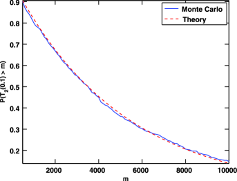
Figure 1: The tail probability $\mathbb{P}\{T_{2}(0.1)>m\}$. Approximate theoretical values are obtained from (17); numerical values are obtained from 500 Monte Carlo trials.

Figure 1 illustrates the fact that $T_{2}(0.1)$ is approximately exponentially distributed.

Results for the EDD obtained from 500 Monte Carlo trials are given in Table 3. Although the approximation seems reasonable, it does not appear to be as accurate as the approximation for the ARL. Since the EDD requires considerably less computational effort to simulate and needs to be known only roughly when we choose design parameters for a particular problem, there is less value to an accurate analytic approximation.

Table 3: EDDs of $T_{2}(p_{0})$ and $T_{4}(p_{0})$ with ARL $\approx 5000$, $\mu=1$, and $m_{1}=200$

$\bolds{p}$	$\bolds{p_{0}}$	Theory $\bolds{T_{2}(p_{0})}$	Monte Carlo $\bolds{T_{2}(p_{0})}$	Theory $\bolds{T_{4}(p_{0})}$	Monte Carlo $\bolds{T_{4}(p_{0})}$
0.3	$0.3$	$3.5$	$3.2$	$4.2$	$3.5$
0.1	$0.3$	$6.2$	$6.5$	$7.1$	$6.6$
0.3	$0.1$	$5.2$	$3.6$	$5.1$	$4.1$
0.1	$0.1$	$7.2$	$6.7$	$7.0$	$7.1$
0.03	$0.1$	$13.9$	$14.3$	$13.5$	$14.3$
0.03	$0.03$	$13.9$	$14.2$	$13.7$	$14.6$

=250pt Procedure $\bolds{b}$ Monte Carlo ARL Max 12.8 5041 $T_{2}(1)$ 53.5 4978 $T_{2}(0.1)$ 19.5 5000 Mei 88.5 4997 $T_{3}(0.1,1)$ 12.4 4948 $T_{3}(1,1)$ 41.6 4993

Table 4: Thresholds for ARL $\approx$ 5000, $m_{1}=200$

Table 5: EDD with $N=100$ obtained from 500 Monte Carlo trials. Thresholds for ARL 5000 are listed in Table 4. Theoretical approximations for EDD are in parentheses

$\bolds{p}$	Method	EDD, $\bolds{\mu=1}$	EDD, $\bolds{\mu=0.7}$	EDD, $\bolds{\mu=1.3}$
0.01	max	25.5	49.6	16.3
	$T_{2}(1)$	52.3 (56.9)	105.5 (114.6)	32.9 (34.1)
	$T_{2}(0.1)$	31.6 (32.5)	59.4 (64.9)	20.3 (19.7)
	Mei	53.2	103.8	38.1
	$T_{3}(0.1,1)$	29.1 (29.3)	63.3 (59.0)	19.1 (19.1)
	$T_{3}(1,1)$	82.0 (83.6)	213.7 (193.5)	53.3 (53.5)
0.03	max	18.1	33.3	11.6
	$T_{2}(1)$	18.7 (19.3)	35.8 (38.4)	12.6 (11.7)
	$T_{2}(0.1)$	14.2 (13.9)	26.7 (27.5)	9.3 (8.5)
	Mei	23.0	41.6	16.4
	$T_{3}(0.1)$	13.4	26.9	9.2
	$T_{3}(1)$	27.2	66.0	16.3
0.05	max	15.5	28.4	9.7
	$T_{2}(1)$	12.2 (11.6)	21.8 (23.0)	7.9 (7.1)
	$T_{2}(0.1)$	10.4 (10.1)	18.9 (19.9)	6.9 (6.2)
	Mei	15.7	26.9	11.4
	$T_{3}(0.1,1)$	9.8 (9.8)	18.6 (21.4)	7.0 (6.8)
	$T_{3}(1,1)$	15.5 (16.2)	38.8 (39.8)	9.0 (9.7)
0.1	max	12.6	23.0	8.4
	$T_{2}(1)$	6.7 (5.9)	11.8 (11.3)	4.7 (3.7)
	$T_{2}(0.1)$	6.7 (7.2)	11.6 (14.1)	4.6 (4.5)
	Mei	9.6	15.4	7.4
	$T_{3}(0.1,1)$	7.1 (7.6)	11.9 (16.7)	5.3 (5.3)
	$T_{3}(1,1)$	6.8 (7.3)	15.7 (19.6)	4.6 (4.5)
0.3	max	9.6	16.7	6.6
	$T_{2}(1)$	3.0 (2.0)	4.4 (3.5)	2.4 (1.4)
	$T_{2}(0.1)$	3.5 (5.2)	5.6 (10.1)	2.7 (3.3)
	Mei	4.9	7.0	4.0
	$T_{3}(0.1,1)$	4.6	6.7	3.9
	$T_{3}(1,1)$	3.0	4.3	2.5
0.5	max	8.6	14.4	5.8
	$T_{2}(1)$	2.3	3.0	2.0
	$T_{2}(0.1)$	2.8	4.0	2.1
	Mei	3.8	5.0	3.0
	$T_{3}(0.1,1)$	4.0	5.4	3.3
	$T_{3}(1,1)$	2.3	3.0	2.0
1	max	7.2	12.1	5.1
	$T_{2}(1)$	2.0	2.0	2.0
	$T_{2}(0.1)$	2.0	2.6	2.0
	Mei	3.0	3.4	2.3
	$T_{3}(0.1,1)$	3.4	4.3	3.0
	$T_{3}(1,1)$	2.0	2.1	2.0

We have performed considerably more extensive simulations that yield results consistent with the small experiments reported in Tables 1, 2 and 3. Since the parameter $p_{0}$ defining $T_{2}$ must be chosen subjectively, it is interesting to observe that Table 3 suggests these procedures are reasonably robust with respect to the choice of $p_{0}$, and choosing $p_{0}$ somewhat too large seems less costly than choosing $p_{0}$ too small. More extensive calculations bear out this observation. We return to the problem of choosing $p_{0}$ in Section 6.

5 Numerical comparisons

In this section, we compare the expected detection delays for several procedures when their ARLs are all approximately 5000. The thresholds are given in Table 4, where we assume $N=100$, and $m_{1}=200$ for those procedures for which a limited window size is appropriate. Procedure (7) is denoted by $T_{2}(p_{0})$. For Mei’s procedure we put $\delta_{n}=1.$ The procedures in (9) are denoted by $T_{3}(p_{0},\delta).$ Recall that $T_{2}(1)$ uses the generalized likelihood ratio statistic and $T_{3}(1,\delta)$ is similar to the procedure proposed by Tartakovsky and Veeravalli TartakovskyVeeravalli2008 , but we have inserted the positive part to avoid the problems mentioned in Section 3. The expected detection delays are obtained from 500 Monte Carlo trials and are listed in Table 5. For some entries, values from our asymptotic approximation are given in parentheses.

Note that the max procedure (8) has the smallest detection delay when $p=0.01$, but it has the largest delay for $p$ greater than 0.1. The procedures defined by $T_{2}$ and by $T_{3}$ are comparable. Mei’s procedure performs well when $p$ is large, but poorly when $p$ is small.

6 Parallel mixture procedure

The procedures considered above depend on a parameter $p_{0}$, which presumably should be chosen to be close to the unknown true fraction $p$. While Table 5 suggests that the value of $p_{0}$ is fairly robust when $p_{0}$ does not deviate much from the true $p$, to achieve robustness over a wider range of the unknown parameter $p$, we consider a parallel procedure that combines several procedures, each using a different $p_{0}$ to monitor a different range of $p$ values. The thresholds of these individual procedures will be chosen so that they have the same ARL. For example, we can use two different values of $p_{0}$, say a small $p_{0}=p_{1}$ and a large $p_{0}=p_{2}$, and then choose thresholds $b_{1}$ and $b_{2}$ to obtain the same ARL for these two procedures. The parallel procedure claims a detection if at least one of the component procedures reaches its threshold, specifically

$$T_{\mathrm{parallel}}\triangleq\min\bigl{\{}T_{2}(p_{1}),T_{2}(p_{2})\bigr{\}}.$$ (35)

To compare the performance of the parallel procedure with that of a single $T_{2}$, we consider a case with $N=400$ and $m_{1}=200$. For the single mixture procedure we use the intermediate value $p_{0}=0.10$ and threshold value $b=44.7$, so $\mathbb{P}^{\infty}\{T_{2}\leq 1000\}\approx 0.10$ and hence the ARL $\approx 10\mbox{,}000$. For the parallel procedure we consider the values $p_{1}=0.02$ and $p_{2}=0.33$. For the threshold values $b_{1}=21.2$ and $b_{2}=87.7$, respectively, we have $\mathbb{P}^{\infty}\{T_{2}(p_{i})\leq 1000\}\approx 0.05$, $i=1,2$. By the Bonferroni inequality $\mathbb{P}^{\infty}\{\min[T_{2}(p_{1}),T_{2}(p_{2})]\leq 1000\}\leq 0.1,$ so conservatively $\mathbb{E}^{\infty}\{T_{\mathrm{parallel}}\}\geq 10\mbox{,}000.$ Table 6 shows that the expected detection delays of the parallel procedure are usually smaller than those of the single procedure, particularly for very small or very large $p$. Presumably these differences are magnified in problems involving larger values of $N$, which have the possibility of still smaller values of $p$.

=250pt $\bolds{p}$ $\bolds{\mu}$ $\bolds{T_{2}(0.1)}$, EDD Parallel, EDD 0.1 0.7 06.5 06.4 0.005 1.0 27.1 22.9 0.005 0.7 54.5 45.8 0.25 0.3 12.0 10.5 0.4 0.2 14.4 12.3 0.0025 1.5 23.3 17.8

Table 6: Comparison of EDD, parallel and simple procedures

Simulations indicate that because of dependence between the two statistics used to define the parallel procedure, the ARL is actually somewhat larger than the Bonferroni approximation suggested. Since the parallel procedure becomes increasingly attractive in larger problems, which provide more room for improvement over a single choice of $p_{0}$, but which are also increasingly difficult to simulate, it would be interesting to develop a more accurate theoretical approximation for the ARL.

An attractive alternative to the parallel procedure would be to use a weighted linear combination for different values of $p_{0}$ of the statistics used to define $T_{2}$ or $T_{3}$. Our approximation for the ARL can be easily adapted, but some modest numerical exploration suggests that the expected detection delay is not improved as much as for the parallel procedure.

7 Profile-based procedure for structured problems

Up to now we have assumed there is no spatial structure relating the change-point amplitudes at difference sensors. In this section we will consider briefly a structured problem, where there is a parameterized profile of the amplitude of the signal seen at each sensor that is based on the distance of the sensor to the source of the signal. Assuming we have some knowledge about such a profile, we can incorporate this knowledge into the definition of an appropriate detection statistic. Our developments follow closely the analysis in SiegmundYakir2008b .

Assume the location of the $n$th sensor is given by its coordinates $x_{n}$, $n=1,\ldots,N$ at points in Euclidean space, which for simplicity we take to be on an equi-spaced grid. We assume that the source is located in a region $\mathcal{D}$, which is a subset of the ambient Euclidean space. In our example below we consider two dimensional space, but three dimensions would also be quite reasonable. Assume the change-point amplitude at the $n$th sensor is determined by the expression

$$\mu_{n}=\sum_{m=1}^{M}r_{m}\alpha_{z_{m}}(x_{n}),$$ (36)

where $M$ is the number of sources, $z_{m}\in\mathcal{D}$ is the (unknown) spatial location of the $m$th source, $\alpha_{z}(x)$ is the profile function, and the scalar $r_{m}$ is an unknown parameter that measures the strength of the $m$th signal. The profile function describes how the signal strength of the $m$th point source has decayed at the $n$th sensor. We assume some knowledge about this profile function is available. For example, $\alpha_{z}(x)$ is often taken to be a decreasing function of the Euclidean distance between $z$ and $x$. The profile may also depend on finitely many parameters, such as the rate of decay of the function. See Rabinowitz1994 or ShafieSigalSiegmund2003 for examples in a fixed sample context.

If the parameters $r_{m}$ are multiplied by a positive constant and the profile $\alpha_{z_{m}}(x_{n})$ divided by the same constant, the values of $\mu_{n}$ do not change. To avoid this lack of identifiability, it is convenient to assume that for all $z$ the profiles have been standardized to have unit Euclidean norm, that is, $\sum_{x}\alpha^{2}_{z}(x)=1$ for all z.

7.1 Profile-based procedure

Under the assumption that there is at most one source, say at $z$, for observations up to time $t$ with a change-point assumed to equal $k$, the log likelihood function for observations from all sensors (1) is

$$\ell(t,k,r,z)=\sum_{n=1}^{N}\bigl{[}r\alpha_{z}(x_{n})(S_{n,t}-S_{n,k})-r^{2}(t-k)\alpha^{2}_{z}(x_{n})/2\bigr{]}.$$ (37)

When maximized with respect to $r$ this becomes

$$\frac{1}{2}\biggl{[}\biggl{\{}\sum_{n}\alpha_{z}(x_{n})U_{n,k,t}\biggr{\}}^{+}\biggr{]}^{2}.$$ (38)

Maximizing the function (38) with respect to the putative change-point $k$ and the source location $z$, we obtain the log GLR statistic and a profile-based stopping rule of the form

$$T_{\mathrm{profile}}=\inf\biggl{\{}t\dvtx\max_{0\leq k<t}\max_{z\in\mathcal{D}}\biggl{[}\biggl{\{}\sum_{n}\alpha_{z}(x_{n})U_{n,k,t}\biggr{\}}^{+}\biggr{]}^{2}\geq b\biggr{\}}.$$ (39)

If the model is correct, (39) is a matched-filter type of statistic.

7.2 Theoretical ARL of profile-based procedure

Using the result presented in SiegmundYakir2008b , we can derive an approximation for the ARL of the profile-based procedure. We consider in detail a special case where $d=2$ and the profile is given by a Gaussian function

$$\alpha_{z}(x)=\frac{1}{\sqrt{2\pi\beta}}e^{-(1/(4\beta))\|x-z\|^{2}},\qquad x\in\mathbb{R}^{2},\beta>0.$$ (40)

The parameter $\beta>0$ controls of rate of profile decay and is assumed known. With minor modifications one could also maximize with respect to a range of values of $\beta$.

Although the sensors have been assumed to be located on the integer lattice of two-dimensional Euclidean space, it will be convenient as a very rough approximation to assume that summation over sensor locations $x$ can be approximated by integration over the entire Euclidean space. With this approximation, $\sum_{x}\alpha^{2}_{z}(x)$, which we have assumed equals 1 for all $z$, becomes $\int_{\mathbb{R}^{2}}\alpha^{2}_{z}(x)\,dx$, which by (40) is readily seen to be identically 1. The approximation is reasonable if $\beta$ is large, so the effective distance between points of the grid is small, and the space ${\mathcal{D}}$, assumed to contain the signal, is well within the set of sensor locations (so edge effects can be ignored and the integration extended over all of ${\mathbb{R}^{2}})$.

It will be convenient to use the notation

$$\langle f,g\rangle=\int_{\mathbb{R}^{2}}f(x)g(x)\,dx.$$ (41)

Let $\dot{\alpha}_{z}$ denote the gradient of $\alpha_{z}$ with respect to $z$. Then according to SiegmundYakir2008b ,

(42)

To evaluate the last integral in (7.2), we see from (40) that $\dot{\alpha}_{z}$ satisfies

$$\dot{\alpha}_{z}(x)=\alpha_{z}(x)(x-z)/(2\beta).$$ (44)

Hence by (41) $\langle\dot{\alpha}_{z},\dot{\alpha}_{z}^{\top}\rangle$ is a $2\times 2$ matrix of integrals, which can be easily evaluated, and its determinant equals $1/(16\beta^{4})$. Hence the last integral in (7.2) equals $|{\mathcal{D}}|/(4\beta^{2})$ where $|{\mathcal{D}}|$ denotes the area of ${\mathcal{D}}$. Arguing as above from the asymptotic exponentiality of $T_{\mathrm{profile}}$, we find that an asymptotic approximation for the average run length is given by

$$\mathbb{E}^{\infty}\{T_{\mathrm{profile}}\}$$

(45)

$$\qquad\sim 16\bigl{(}2\pi^{3}\bigr{)}^{1/2}\beta^{2}b^{-3/2}\exp(b/2)\Big{/}\biggl{[}\int_{(b/m_{1})^{1/2}}^{(b/m_{0})^{1/2}}u\nu^{2}(u)\,du\cdot|{\mathcal{D}}|\biggr{]}.$$

7.3 Numerical examples

In this section we briefly compare the unstructured detection procedure based on $T_{2}$ with the profile-based procedure in the special case that the assumed profile is correct.

Assume that the profile is given by the Gaussian function (40) with parameter $\beta=1$ and both procedures are window-truncated with $m_{0}=1$, $m_{1}=100$. The number of sensors is $N=625$ distributed over a $25\times 25$ square grid with center at the origin. In this situation, approximately $p=0.016$ sensors are affected. In the specification of $T_{2}$, we take $p_{0}=0.05$.

The thresholds are chosen so that the average run lengths when there is no change-point are approximately 5000. Using (7.2), we obtain $\mathbb{P}^{\infty}\{T_{\mathrm{profile}}\leq 250\}=0.050$ for $b=29.5$. From 500 Monte Carlo trials we obtained the threshold 26.3, so the theoretical approximation appears to be slightly conservative.

To deal with a failure to know the true rate of decay of the signal with distance, we could maximize over $\beta$, say, for $\beta\in[0.5,5]$. A suitable version of (7.2) indicates the threshold would be 33.8. This slight increase to the threshold suggests that failure to know the appropriate rate of decay of the signal with distance leads to a relatively moderate loss of detection efficiency.

=265pt $\bolds{b}$ EDD $\bolds{r=1}$ EDD, $\bolds{r=1.5}$ Profile-based procedure 26.3 25.6 12.3 Unstructured procedure 39.7 78.3 35.8

Table 7: Comparison of EDD, profile-based and unstructured procedures

For comparisons of the EDD, we used for the profile-based procedure the threshold 26.3, given by simulation, while for $T_{2}(0.05)$ we used the analytic approximation, which our studies have shown to be very accurate. Table 7 compares the expected detection delay of the profile-based procedure with that of the mixture procedure. As one would expect from the precise modeling assumptions, the profile-based procedure is substantially more powerful.

In many cases there will be only a modest scientific basis for the assumed profile, especially in multidimensional problems. The distance between sensors relative to the decay rate of the signal is also an important consideration. It would be interesting to compare the structured and the unstructured problems when the assumed profile differs moderately or substantially from the true profile, perhaps in the number of sources of the signals, their shape, the rate of decay, or the locations of the sensors.

8 Discussion

For an unstructured multi-sensor change-point problem we have suggested and compared a number of sequential detection procedures. We assume that the pre- and post-change samples are normally distributed with known variance and that both the post-change mean and the set of affected sensors are unknown. For performance analysis, we have derived approximations for the average run length (ARL) and the expected detection delay (EDD), and have shown that these approximations have reasonable accuracy. Our principal procedure depends on the assumption that a known fraction of sensors are affected by the change-point. We show numerically that the procedures are fairly robust with respect to discrepancies between the actual and the hypothesized fractions, and we suggest a parallel procedure based on two or more hypothesized fractions to increase this robustness.

In a structured problem, we have shown that knowledge of the correct structure can be implemented to achieve large improvements in the EDD. Since the assumed structure is usually at best only approximately correct, an interesting open question is the extent to which failure to hypothesize the appropriate structure compromises these improvements. One possible method to achieve robustness against inadequacy of the structured model would be a parallel version of structured and unstructured detection.

References

- (1) {bbook}[mr] \bauthor\bsnmAldous, \bfnmDavid\binitsD. (\byear1989). \btitleProbability Approximations Via the Poisson Clumping Heuristic. \bseriesApplied Mathematical Sciences \bvolume77. \bpublisherSpringer, \blocationNew York. \bidmr=0969362 \bptnotecheck year\bptokimsref \endbibitem
- (2) {barticle}[auto] \bauthor\bsnmChen, \bfnmM.\binitsM., \bauthor\bsnmGonzalez, \bfnmS.\binitsS., \bauthor\bsnmVasilakos, \bfnmA.\binitsA., \bauthor\bsnmCao, \bfnmH.\binitsH. and \bauthor\bsnmLeung, \bfnmV. C. M.\binitsV. C. M. (\byear2010). \btitleBody area networks: A survey. \bjournalMobile Netw. Appl. \bvolume16 \bpages171–193. \bptokimsref \endbibitem
- (3) {barticle}[mr] \bauthor\bsnmLai, \bfnmTze Leung\binitsT. L. (\byear1995). \btitleSequential changepoint detection in quality control and dynamical systems. \bjournalJ. Roy. Statist. Soc. Ser. B \bvolume57 \bpages613–658. \bidissn=0035-9246, mr=1354072 \bptnotecheck related\bptokimsref \endbibitem
- (4) {barticle}[mr] \bauthor\bsnmLévy-Leduc, \bfnmCéline\binitsC. and \bauthor\bsnmRoueff, \bfnmFrançois\binitsF. (\byear2009). \btitleDetection and localization of change-points in high-dimensional network traffic data. \bjournalAnn. Appl. Stat. \bvolume3 \bpages637–662. \biddoi=10.1214/08-AOAS232, issn=1932-6157, mr=2750676 \bptokimsref \endbibitem
- (5) {barticle}[mr] \bauthor\bsnmLorden, \bfnmG.\binitsG. (\byear1971). \btitleProcedures for reacting to a change in distribution. \bjournalAnn. Math. Statist. \bvolume42 \bpages1897–1908. \bidissn=0003-4851, mr=0309251 \bptokimsref \endbibitem
- (6) {barticle}[mr] \bauthor\bsnmMei, \bfnmY.\binitsY. (\byear2010). \btitleEfficient scalable schemes for monitoring a large number of data streams. \bjournalBiometrika \bvolume97 \bpages419–433. \biddoi=10.1093/biomet/asq010, issn=0006-3444, mr=2650748 \bptokimsref \endbibitem
- (7) {barticle}[mr] \bauthor\bsnmPage, \bfnmE. S.\binitsE. S. (\byear1954). \btitleContinuous inspection schemes. \bjournalBiometrika \bvolume41 \bpages100–115. \bidissn=0006-3444, mr=0088850 \bptokimsref \endbibitem
- (8) {barticle}[mr] \bauthor\bsnmPage, \bfnmE. S.\binitsE. S. (\byear1955). \btitleA test for a change in a parameter occurring at an unknown point. \bjournalBiometrika \bvolume42 \bpages523–527. \bidissn=0006-3444, mr=0072412 \bptokimsref \endbibitem
- (9) {bbook}[auto] \bauthor\bsnmPetrov, \bfnmA.\binitsA., \bauthor\bsnmRozovskii, \bfnmB. L.\binitsB. L. and \bauthor\bsnmTartakovsky, \bfnmA. G.\binitsA. G. (\byear2003). \btitleEfficient Nonlinear Filtering Methods for Detection of Dim Targets by Passive Systems, Vol. IV. \bpublisherArtech House, \blocationBoston, MA. \bptokimsref \endbibitem
- (10) {barticle}[mr] \bauthor\bsnmPollak, \bfnmM.\binitsM. and \bauthor\bsnmSiegmund, \bfnmD.\binitsD. (\byear1975). \btitleApproximations to the expected sample size of certain sequential tests. \bjournalAnn. Statist. \bvolume3 \bpages1267–1282. \bidissn=0090-5364, mr=0403114 \bptokimsref \endbibitem
- (11) {bincollection}[mr] \bauthor\bsnmRabinowitz, \bfnmDaniel\binitsD. (\byear1994). \btitleDetecting clusters in disease incidence. In \bbooktitleChange-point Problems (South Hadley, MA, 1992). \bseriesInstitute of Mathematical Statistics Lecture Notes—Monograph Series \bvolume23 \bpages255–275. \bpublisherIMS, \blocationHayward, CA. \biddoi=10.1214/lnms/1215463129, mr=1477929 \bptokimsref \endbibitem
- (12) {barticle}[mr] \bauthor\bsnmShafie, \bfnmK.\binitsK., \bauthor\bsnmSigal, \bfnmB.\binitsB., \bauthor\bsnmSiegmund, \bfnmD.\binitsD. and \bauthor\bsnmWorsley, \bfnmK. J.\binitsK. J. (\byear2003). \btitleRotation space random fields with an application to fMRI data. \bjournalAnn. Statist. \bvolume31 \bpages1732–1771. \biddoi=10.1214/aos/1074290326, issn=0090-5364, mr=2036389 \bptokimsref \endbibitem
- (13) {bbook}[mr] \bauthor\bsnmSiegmund, \bfnmDavid\binitsD. (\byear1985). \btitleSequential Analysis: Tests and Confidence Intervals. \bpublisherSpringer, \blocationNew York. \bidmr=0799155 \bptokimsref \endbibitem
- (14) {barticle}[mr] \bauthor\bsnmSiegmund, \bfnmD.\binitsD. and \bauthor\bsnmVenkatraman, \bfnmE. S.\binitsE. S. (\byear1995). \btitleUsing the generalized likelihood ratio statistic for sequential detection of a change-point. \bjournalAnn. Statist. \bvolume23 \bpages255–271. \biddoi=10.1214/aos/1176324466, issn=0090-5364, mr=1331667 \bptokimsref \endbibitem
- (15) {bbook}[mr] \bauthor\bsnmSiegmund, \bfnmDavid\binitsD. and \bauthor\bsnmYakir, \bfnmBenjamin\binitsB. (\byear2007). \btitleThe Statistics of Gene Mapping. \bpublisherSpringer, \blocationNew York. \bidmr=2301277 \bptokimsref \endbibitem
- (16) {barticle}[mr] \bauthor\bsnmSiegmund, \bfnmDavid\binitsD. and \bauthor\bsnmYakir, \bfnmBenjamin\binitsB. (\byear2008). \btitleDetecting the emergence of a signal in a noisy image. \bjournalStat. Interface \bvolume1 \bpages3–12. \bidissn=1938-7989, mr=2425340 \bptokimsref \endbibitem
- (17) {barticle}[mr] \bauthor\bsnmSiegmund, \bfnmDavid\binitsD., \bauthor\bsnmYakir, \bfnmBenjamin\binitsB. and \bauthor\bsnmZhang, \bfnmNancy R.\binitsN. R. (\byear2011). \btitleDetecting simultaneous variant intervals in aligned sequences. \bjournalAnn. Appl. Stat. \bvolume5 \bpages645–668. \biddoi=10.1214/10-AOAS400, issn=1932-6157, mr=2840169 \bptokimsref \endbibitem
- (18) {barticle}[mr] \bauthor\bsnmŠirjaev, \bfnmA. N.\binitsA. N. (\byear1963). \btitleOptimal methods in quickest detection problems. \bjournalTheory Probab. Appl. \bvolume8 \bpages22–46. \bptokimsref \endbibitem
- (19) {barticle}[mr] \bauthor\bsnmTartakovsky, \bfnmAlexander G.\binitsA. G. and \bauthor\bsnmVeeravalli, \bfnmVenugopal V.\binitsV. V. (\byear2008). \btitleAsymptotically optimal quickest change detection in distributed sensor systems. \bjournalSequential Anal. \bvolume27 \bpages441–475. \biddoi=10.1080/07474940802446236, issn=0747-4946, mr=2460208 \bptokimsref \endbibitem
- (20) {bmisc}[auto] \bauthor\bsnmXie, \bfnmY.\binitsY. (\byear2011). \bhowpublishedStatistical signal detection with multi-sensor and sparsity. Ph.D. thesis, Stanford Univ. \bptokimsref \endbibitem