Macroscopic magnetic frustration

Abstract

Although geometrical frustration transcends scale, it has primarily been evoked in the micro and mesoscopic realm to characterize such phases as spin-ice liquids and glasses and to explain the behavior of such materials as multiferroics, high temperature superconductors, colloids and copolymers. Here we introduce a system of macroscopic ferromagnetic rotors arranged in a planar lattice capable of out-of-plane movement that exhibit the characteristic honeycomb spin ice rules studied and seen so far only in its mesoscopic manifestation. We find that a polarized initial state of this system settles into the honeycomb spin ice phase with relaxation on multiple time scales. We explain this relaxation process using a minimal classical mechanical model which includes Coulombic interactions between magnetic charges located at the ends of the magnets and viscous dissipation at the hinges. Our study shows how macroscopic frustration arises in a purely classical setting that is amenable to experiment, easy manipulation, theory and computation, and shows phenomena that are not visible in their microscopic counterparts.

Frustration in physical systems commonly arises because geometrical or topological constraints prevent global energy minima from being realized. Although not limited to microscopic phenomena, it is commonly seen in compounds with spins forming lattices with a triangular motif Diep (2004). In such systems, frustration may lead to the existence of ice selection rules Petrenko and Whitworth (1999) which have been observed in a variety of materials where spins form networks such as the corner-sharing tetrahedra, known as the Pyrochlore lattice Ramirez et al. (1999); Gingras (2011); Gardner et al. (2010), leading to monopole-like excitations Castelnovo et al. (2008) and other exotic phases of matter Powell (2011). Even though, artificial spin ices Tanaka et al. (2006); Qi et al. (2008); Wang et al. (2006) have shown that frustration can be mimicked by classical magnets, these systems do not account quantitatively for the effects of inertia, dissipation Han et al. (2008); Thomas et al. (2010); Irvine et al. (2010), dilution and geometrical disorder because of the mesoscopic scale and fast dynamics of the domain walls ($\sim 10$ ns) that hinder the understanding of collective dynamics processes. Here we aim to circumvent this situation by introducing a new macroscopic realization of a frustrated magnetic system created using single out-of-plane rotational degree of freedom magnetic rotors, arranged in a kagome lattice, a pattern of corner-sharing triangular plaquettes that dynamically evolves into a spin-ice phase after a magnetic quench. The ice phase is reached due to the delicate interplay between inertia, friction and Coulomb-like interactions between the macroscopic magnetic rods. Our prototypical frustrated system has a few advantages for research in frustrated magnetic systems associated with the ability to (i) tune the interactions through changes in distance and/or orientation between magnets and (ii) examine the lattice relaxation dynamics by direct visualization at a single particle level.

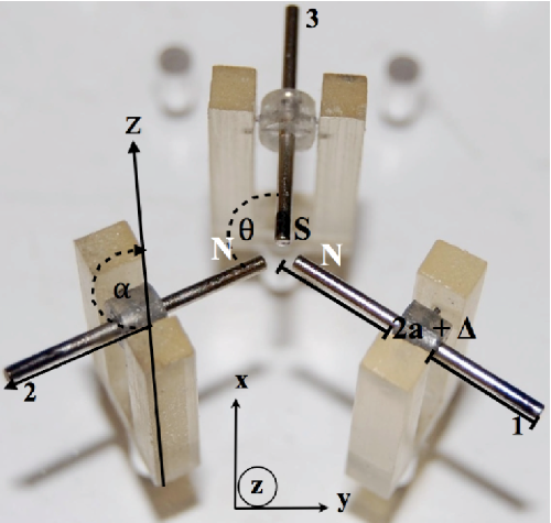
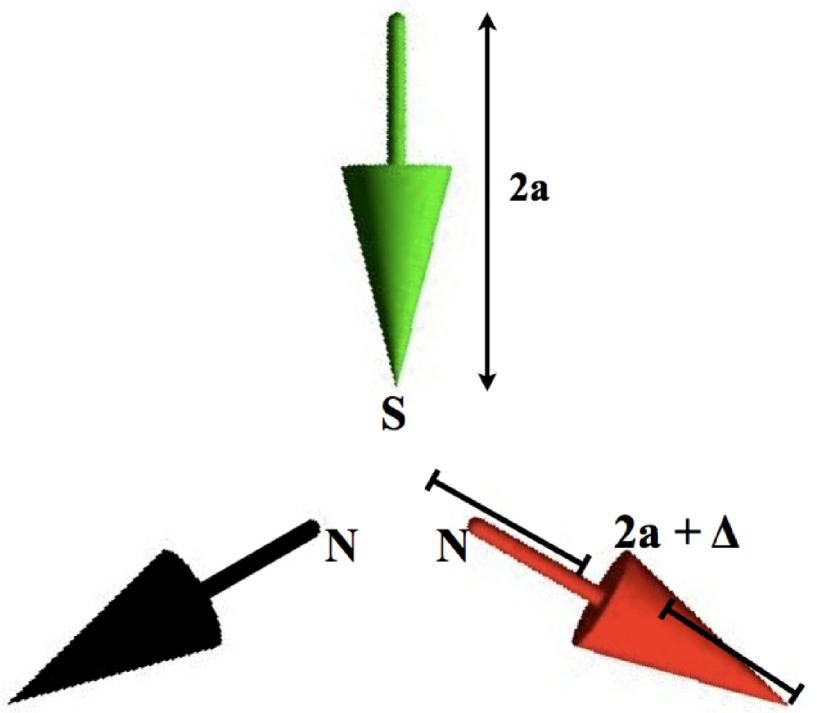
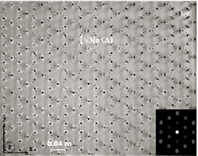
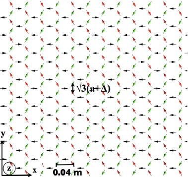
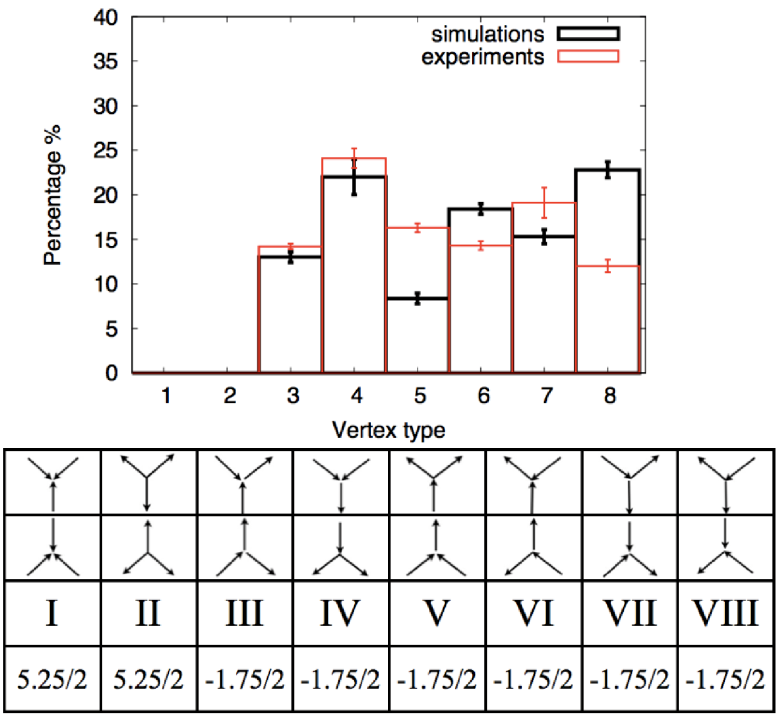
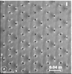
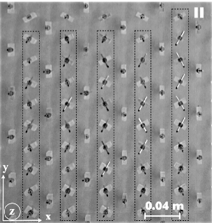
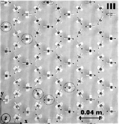
A minimal macroscopic realization of local frustration can be seen easily in a $120^{\circ}$ star configuration using three ferromagnetic rods with their hinges on a plane (Fig. 1a). The rods have length $L=2a=1.9\times 10^{-2}$ m, diameter $d=1.5\times 10^{-3}$ m, mass $M=0.28\times 10^{-3}$ Kg and saturation magnetization $M_{s}=1.2\times 10^{6}$ A $m^{-1}$. By design the only allowed motions for the rotors are rotations in the polar direction $\alpha$. The hinges supporting the rods were placed at the sites of a kagome lattice with lattice constant $l=\sqrt{3}(a+\Delta)$ where $\Delta$ is the shortest distance between the tips and the nearest vertex center and $\Delta/L\sim 0.2$ (Fig. 1a), so that when in the $x-y$ plane, the magnets realize the bonds of a honeycomb lattice. The magnetization of a rotor $i$ is defined as the vector $\mathbf{m_{i}}$ joining its N to its S pole, thus $\mathbf{m_{i}}$ is the coarse-grained spin variable for each magnet. When all three magnets are close to each other, the lowest energy configuration consists of one pole being different from the others, leading to a frustrated state consisting of permutations of NNS or SSN (S=south pole, N = north pole) that correspond to the honeycomb spin ice rules Qi et al. (2008); Mellado et al. (2010). With this unit-cell plaquette, we prepare a polarized lattice of $n=352$ of these magnetic rotors, with an unavoidable geometrical disorder in the azimuthal orientation of the rotors, $\theta$, due to lattice imperfections $\delta\theta_{\rm{max}}\sim 2^{o}$; this follows a Gaussian distribution with mean $\bar{\delta\theta}=1.2^{\circ}$. We oriented the S poles of all rotors out of the plane by applying a strong magnetic field along the $\hat{z}$ direction $B_{z}=3.2\times 10^{-3}$ T (Supplementary Information S4). At $t=0$ the field was switched off, to allow for the lattice to relax, a procedure that was repeated several times. After about 2 seconds, all the rotors had reached equilibrium configurations very near the $x-y$ plane (the non-planarity out of the $x-y$ plane $\delta\alpha\sim 10^{\circ}$ on average) and in the honeycomb spin ice manifold. Figure 1e, shows a picture of the lattice where all the rods fulfill the ice rules. The experimental distribution of vertices is shown in the (red) bars of Figure 1c. We find all vertices falling into the six low energy (spin ice) configurations while high energy states (type 1 and 2) are absent.

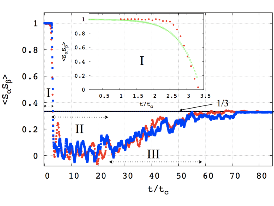
This macroscopic spin ice consists of elemental rotor units that constitute a frustrated triad which we characterize at a static and a dynamic level (Supplementary Information S1, S2 and S3). This allows us to use a dipolar dumbbell approach to the magnets Castelnovo et al. (2008), determine the charge $q=\pi M_{s}d^{2}/4\sim 2.03$ A m, at each pole, find the damping time scale for an isolated rod $\tau_{D}\sim 1$ s and examine how Coulomb interactions and geometrical disorder in $\theta$ and $\Delta$ control the orientations of the rods relative to each other. On a collective level, the relaxation of the lattice from the $\hat{z}$ polarized state to the spin ice manifold may be characterized in terms of the correlation between nearest neighbor spins $\alpha$ and $\beta$, with $S_{\alpha}S_{\beta}=1$ when $\mathbf{m_{\alpha}}\cdot\mathbf{m_{\beta}}$ is positive, $S_{\alpha}S_{\beta}=-1$ otherwise. From high speed movies (400 fps), we extracted the full time trajectory $\alpha_{i}(t)$ of the $i-th$ rotor (Supplementary S4 and Movie MS1) and computed the spin-spin correlations.

We find that there are three stages in the spin relaxation process. In stage I, corresponding to the first $\sim 0.07$ s, the rotors break their initial axial symmetry, Figure 2a, and correlations decay rapidly with a characteristic Coulomb time scale $t_{c}\sim 0.02$ s, Figure 2d, which is the shortest time scale in the lattice relaxation, with $t_{c}\sim\frac{\sqrt{aI/\mu_{0}}}{q}$ dominated by internal Coulomb interactions for the relaxation of a rotor interacting with two neighbors (Supplementary S4) in the absence of damping and external torques (inset of Figure 2d). Next, magnets of sub-lattices 1 and 2 (Fig.1a) organize in head to tail chains along the $\hat{y}$ direction, while those belonging to sub-lattice 3 still remain non-planar, Figure 2b. In Stage II, once the sub-lattice 3 becomes planar, all the rods spin continuously leading to a plateau in the spin correlations (Fig.2d); eventually the kinetic energy of the rotors has been dissipated sufficiently that the rotors oscillate rather than spin. For our experimental parameters (Fig.1a), the phase space trajectory changes from librations to damped oscillations after $0.45$ s (Supplementary Fig. S7); the rotors typically average about four full rotations before they switch to oscillations. Finally, in Stage III (Fig.2c and Fig.2d) the rods oscillate without full rotations: when we fit the experimental dynamics at this state to a decaying exponential we find $t_{d}\sim\tau_{D}$, thus this stage is dominated by dissipative effects.

To understand these different dynamical regimes, we performed molecular dynamics simulations of the massive underdamped rotors interacting through the full long-range internal Coulomb interactions between all the rods in the lattice using a Verlet algorithm (Supplementary S5, Fig.S10 and Movie SM2). In Figure 2d, we see that the computed nearest neighbor spin correlations for the relaxation of the numerical lattice has the same three qualitative different regimes as in the experiments when the lattice relaxes from a polarized state to its spin ice manifold. Furthermore, the Coulomb and damping time scales for stage I and III as well as the plateau featuring stage II are in good agreement with experiments. The observed high frequency fluctuations in $\langle S_{\alpha}S_{\beta}\rangle(t)$ in both, experiments and simulations, are due to the Coulomb coupling between rods which rapidly reorient while they relax due to the fluctuations in the internal magnetic field.

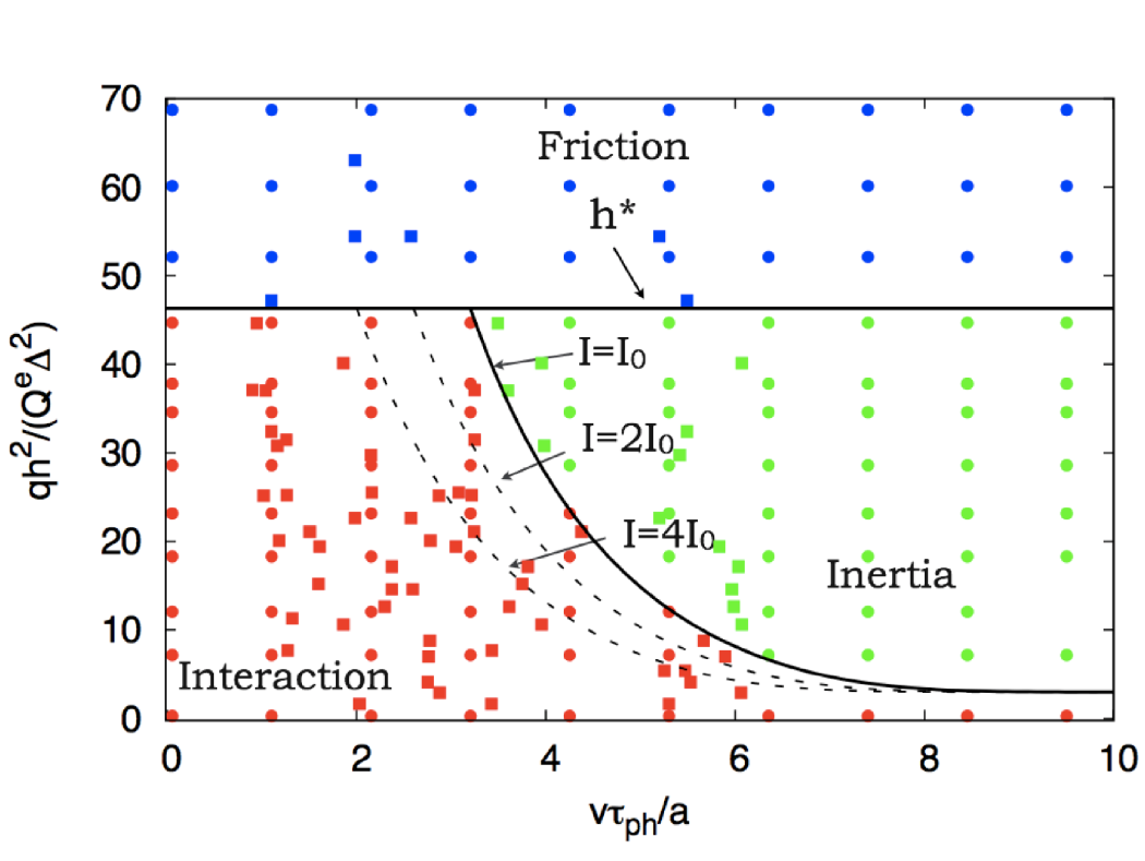
Having examined the dynamics of relaxation to the spin ice state, we now turn to the lattice response when a dipole with charge $|Q^{e}|$ at each pole and length $L^{e}$, at a vertical distance $h$ underneath the relaxed lattice is moved along one of the three sub-lattices at speed $v$ (Supplementary Fig.S9). For an isolated rotor, the critical torque that is required to destabilize the planar configuration is given by $\mathit{T_{c}}\sim 2aB_{c}q$, where $B_{c}$ is the applied magnetic field; experiments on many rotors yielded an average $B_{c}\sim(2.4\pm 0.1)\times 10^{-4}$ T. Equivalently, the threshold distance at which the external field will overcome both internal Coulomb interactions and static friction is given by $h^{*}\sim\sqrt{Q^{e}qa/\mathit{T_{c}}}$. Dynamically, the internal Coulomb interactions set a time scale for small out-of-plane oscillations of the rotors in the lattice, given by $\tau_{ph}\sim\sqrt{\Delta^{2}I/\mu_{0}q^{2}a}\sim 0.01s$ for the experimental parameters at hand. Thus, there are two dimensionless quantities that determine the response to the external perturbation: the ratio between phononic and kinetic time scales $v\tau_{ph}/a$ and the ratio between internal and external magnetic forces, $F^{int}/F^{ext}=qh^{2}/(Q^{e}\Delta^{2})$.

In Figure 3, we characterize the phase diagram of the dynamical response of the spin-ice lattice in terms of these dimensionless parameters. For $h<h^{*}$, the lattice is disturbed only in a band of width $D(h)\sim\sqrt{(h^{*2}h)^{2/3}-h^{2}}$ centered along the trajectory of the moving external dipole, based only on local interactions, static friction, and interactions with the external dipole (Supplementary Fig.S9). For large $v$, $\tau_{ph}/\tau_{k}\gg 1$ so that the rotors have little time to respond and barely oscillate in an inertia-dominated regime. In the opposite limit, large amplitude oscillations and flips are apparent as there is enough time for the rotors to interact with the external dipole. Our results for these regimes show that the simulations (filled circles) and experiments (filled squares) agree. The solid line defines a threshold of the RMS fluctuations for the oscillations of all the rods $\delta_{Li}^{th}=0.5$ (Supplementary S4) separating the regimes. To understand this, we resort to a simple single rod approximation where the impulsive response of a rotor due to a long dipole located at a distance $d(t)=\sqrt{h^{2}+(vt)^{2}}$, balances the change in its angular momentum yielding $h\sim h^{*}(Q^{e}qa/I)^{3/2}/v^{3}$, consistent with the observations when $v\tau_{ph}/a\gg 1$. Varying inertia from $I_{0}$ to $4I_{0}$ using our simulations we confirmed that as $I$ grows, the boundary between interaction and inertial regime shift to the left; the inertial regime is reached for smaller values of $v\tau_{ph}/a$ and $qh^{2}/(Q^{e}\Delta^{2})$. When $h\gg h^{*}$, the Coulomb force due to the external field is not able to overcome the combined effects of static friction and internal Coulomb interactions, and the lattice falls into a friction dominated one in which oscillations are not apparent.

Our spin ice phase emerges in a system of damped macroscopic rotors, purely driven by interactions in a classical mechanical setting that differs from those found in its micro and mesoscopic relatives. Using a minimal model we can capture the dynamical evolution of the collection of rotors in the lattice observed in our experiments and reproduce the three main stages of lattice relaxation from a polarized state: explosive behavior lasting $t_{c}$, dissipative librations and damped oscillations. The advantages of studying this macroscopic realization beyond the present work include the fact that (i) the interactions can be tuned through changes in the diameter of magnets or distance or orientation between them (Supplementary Fig. S4), (ii) inertial and dissipative effects can be studied by controlling the friction coefficient at the hinges as well as the mass of the rods, (iii) the effect of vacancies or random dilution can be examined by removing rotors from the lattice (iv) the lattice relaxation dynamics can be directly visualized at single particle level and (v) the system can be easily generalized to three dimensions (3-D) by stacking plates with hinged rotors along the $z$ direction. Indeed a minimal 3-D realization is shown in Supplementary Fig. S12: a tetrahedral configuration like the one found in the Pyrochlore lattice was created placing three acrylic plates one on the top of the other, the bottom and top plates contain three rotors defining an equilateral triangle and the middle plate contains one rotor located equidistant from the others. The ease of fabrication, manipulation and measurement and the study of a variety of soft modes in artificial lattices in a system that is nearly five orders of magnitude larger and slower than its mesoscopic counterpart suggests that there is a new class of phenomena waiting to be explored in macroscopic frustrated systems.

Figure 1: The unit cell star configuration and the honeycomb lattice of magnetic rotors in the spin ice manifold. $\mathbf{a,}$ A triad of magnetic rotors (lying in one of the sublattices indicated as 1, 2 and 3) having length $L=2a=1.9\times 10^{-2}$ m, diameter $d=1.5\times 10^{-3}$ m, mass $M=0.28\times 10^{-3}$ Kg and saturation magnetization $M_{s}=1.2\times 10^{6}$ A $m^{-1}$ are located at $\theta=120^{\circ}$ respect to each other. The out of plane degree of freedom is denoted by the polar angle $\alpha$. Painted in black the magnet south pole (S) is distinguished from its north pole (N). $\mathbf{b,}$ The numerical equivalent magnetic triad having the same experimental parameters. In this case the point of the arrow denotes the S pole. $\mathbf{c,}$ Picture of the lattice with its centers located at distance $l=\sqrt{3}(a+\Delta)$ with the n rods lying in the $x-y$ plane fulfilling the honeycomb spin ice rules. Inset shows the Fourier transform of the lattice. $\mathbf{d,}$ The numerical equivalent lattice with same parameters as the experimental one. $\mathbf{e,}$ Up: Histograms taken from 10 experiments and simulations showing the experimental (red) and numerical (black) distribution of vertices. Bottom: Table with the local energy of the eight vertex configurations possible in the honeycomb lattice, in units of $D=10^{-5}$ J (Supplementary S6).

Figure 2: Lattice dynamics characterized by nearest neighbor spin correlations, $\langle S_{\alpha}S_{\beta}\rangle$. $\mathbf{a,}$ Stage I: once $B_{z}$ is turned off, the rotors originally pointing along $\hat{z}$ break their axial symetry. $\mathbf{b,}$ with the image showing the end of stage I and the onset of stage II when rods rotate respect to their center of mass yielding a plateau in $\langle S_{\alpha}S_{\beta}\rangle$. $\mathbf{c,}$ with a snapshot of the rods oscillating in stage III. $\mathbf{d,}$ In red experimental data obtained via image processing, in blue molecular dynamics simulation results from the numerical solution of equation (S4) where the full coulomb contributions from all neighbors is taken into account. At t=0 all S poles point along $\hat{z}$. Stage I is dominated by Coulomb interactions between rods and characterized by the Coulomb time scale $t_{c}$. In Stage II, all rotors spin until dissipation damps out the spin in favor of oscillations, leading to Stage III where they exhibit damped oscillations. After relaxation the rods lie in the x-y plane in a honeycomb spin ice magnetic configuration, with its characteristic nearest neighbor spin correlations $\langle S_{\alpha}S_{\beta}\rangle=1/3$ (solid line). Inset: Experimentally measured value of $\langle S_{\alpha}S_{\beta}\rangle$ during the initial explosive evolution (red) compared with $\cos(\alpha)$ where $\alpha$ is the solution of Supplementary equation (S2) for one rotor interacting with two neighbors, in the absence of damping and external torques (green).

Figure 3: Phase diagram of the lattice dynamical response to an external perturbation. The horizontal axis shows the dimensionless ratio of the kinetic and phononic time scales with $v$ the speed of an external dipole, while the vertical axis shows the dimensionless ratio of the internal and the external magnetic forces due to an external dipole of strength $Q$ located at distance $h$ from the lattice (see text for details). Experimental and numerical data shown in squares and circles respectively, and colors define the nature of the lattice dynamical response to the external perturbation. We see that the dynamics may be broken up into a frictionally dominated, interaction dominated or inertially dominated regime as a function of the relative magnitude and rate of external forcing.

References

- Diep (2004) H. T. Diep, ed., Frustrated Spin Systems (World Scientific, 2004).
- Petrenko and Whitworth (1999) V. F. Petrenko and R. W. Whitworth, Physics of Ice (Oxford University Press, 1999).
- Ramirez et al. (1999) A. P. Ramirez, A. Hayashi, R. J. Cava, R. Siddharthan, and B. S. Shastry, Nature 399, 333 (1999).
- Gingras (2011) M. J. P. Gingras, in Introduction to Frustrated Magnetism, edited by C. Lacroix, P. Mendels, and F. Mila (Springer Verlag, 2011).
- Gardner et al. (2010) J. S. Gardner, M. J. P. Gingras, and J. E. Greedan, Rev. Mod. Phys. 82, 53 (2010).
- Castelnovo et al. (2008) C. Castelnovo, R. Moessner, and S. L. Sondhi, Nature 451, 42 (2008).
- Powell (2011) S. Powell, Phys. Rev. B 84, 094437 (2011).
- Tanaka et al. (2006) M. Tanaka, E. Saitoh, H. Miyajima, T. Yamaoka, and Y. Iye, Phys. Rev. B 73, 052411 (2006).
- Qi et al. (2008) Y. Qi, T. Brintlinger, and J. Cumings, Phys. Rev. B 77, 094418 (2008).
- Wang et al. (2006) R. F. Wang, C. Nisoli, R. S. Freitas, J. Li, W. McConville, B. J. Cooley, M. S. Lund, N. Samarth, C. Leighton, V. H. Crespi, et al., Nature 439, 303 (2006).
- Han et al. (2008) Y. Han, Y. Shokef, A. M. Alsayed, P. Yunker, T. C. Lubensky, and A. G. Yodh, Nature 456, 898 (2008).
- Thomas et al. (2010) L. Thomas, R. Moriya, C. Rettner, and S. S. P. Parkin, Science 330, 1810 (2010).
- Irvine et al. (2010) W. T. M. Irvine, V. Vitelli, and P. M. Chaikin, Nature 468, 947 (2010).
- Mellado et al. (2010) P. Mellado, O. Petrova, Y. Shen, and O. Tchernyshyov, Phys. Rev. Lett. 105, 187206 (2010).