MMANOVA: A general multilevel framework for multivariate analysis of variance

Abstract Classical analysis of variance requires that model terms be labeled as fixed or random and typically culminate by comparing variability from each batch (factor) to variability from errors; without a standard methodology to assess the magnitude of a batch’s variability, to compare variability between batches, nor to consider the uncertainty in this assessment. In this paper we support recent work, placing ANOVA into a general multilevel framework, then refine this through batch level model specifications, and develop it further by extension to the multivariate case. Adopting a Bayesian multilevel model parametrization, with improper batch level prior densities, we derive a method that facilitates comparison across all sources of variability. Whereas classical multivariate ANOVA often utilizes a single covariance criterion, e.g. determinant for Wilks’ lambda distribution, the method allows arbitrary covariance criteria to be employed. The proposed method also addresses computation. By introducing implicit batch level constraints, which yield improper priors, the full posterior is efficiently factored, thus alleviating computational demands. For a large class of models, the partitioning mitigates, or even obviates the need for methods such as MCMC. The method is illustrated with simulated examples and an application focusing on climate projections with global climate models.

Keywords:  Bayesian inference; Constraints; Mixed model; Variance components

1 Introduction

Identifying and comparing variability among several factors is a fundamental task of statistical analysis. From initial exploratory steps, to model testing, analysis of variance plays a vital role in the practice of statistics. Gelman, (2005) has outlined a general ANOVA methodology that fits a wide range of models and summarizes results in a manner that facilitates interpretation across different sources of variation. Gelman and Hill, (2006) elaborate further, describing the methodology in terms of a multilevel model. One important contribution of this approach is in providing summaries that are more constructive than conclusions based on hypothesis tests. This framework is seeing usage by researchers from diverse fields e.g. ecology (Qian and Shen,, 2007), genetics (Leinonen et al.,, 2008), and climate (Sain et al.,, 2011).

This paper presents a method that adopts the multilevel approach towards ANOVA, then extends it to multivariate settings, yielding a multilevel multivariate analysis of variance (MMANOVA) methodology. The strategy of initially treating all sources of variability in similar regard is naturally a part of the new method. We address known issues of applying constraints in variance analyses (Nelder,, 1977, 1994, 1999) by constraining batch levels so that prior distributions are improper. The extension is seen as a valuable contribution, since multivariate ANOVA can further obfuscate model specification, interpretation, and computation. Kaufman and Sain, (2010) offer an analysis of variance procedure that aids in model specification and interpretation, but requires computationally demanding MCMC steps. Recent methods involving approximations, e.g. integrated nested Laplace approximations (INLA) (Lindgren et al.,, 2011; Rue et al.,, 2009), have allowed for MCMC to be eliminated in many cases, significantly reducing computational demands. While the range of problems for which such methods are applicable is wide, the focus is not typically on variance parameters. Thus, the contribution of our work is in promoting a general ANOVA methodology. We accomplish this by supporting recent work with the same goal, by refining the model specification, and by extending this to multivariate cases.

In Section 2 we review the ANOVA formulation of Gelman, (2005) and summarize some details of the approach. We then formally extend the idea to the multivariate case, discussing technical and computational aspects. Section 3 provides a demonstration of the method through a simulation example and through a climatological application using data from future climate projections given by several atmosphere-ocean general circulation models and global emissions scenarios. In Section 4 we discuss extensions and further computational benefits that are possible when the method is applied to common high-dimensional problems.

2 Analysis of Variance

Analysis of variance is widely accepted as a means of partitioning variability in a manner which allows it to be attributed to various factors. An important initial step in the analysis is considering each factor of the model to be fixed or random. This step, necessary in the classical setting, raises enough issues that statisticians have been obliged to address the “mixed models controversy” (Lencina et al.,, 2005; Voss,, 1999). One might conclude that a consensus has still not been reached, given that John Nelder deemed it necessary to reiterate the requisite points of constraints and marginality over such a long period of time, beginning with Nelder, (1977) and most recently Nelder, (2008).

The rest of the section outlines a recent attempt by Gelman, (2005) towards a more universal ANOVA methodology, then refines and extends the approach to a multivariate context.

2.1 Multilevel ANOVA

A fundamental contribution of the hierarchical regression approach to ANOVA employed by Gelman, (2005) has been to indiscriminately consider all components in a model as random, thereby facilitating comparison across all sources of variability. The terminology is useful in supporting the indiscriminate nature of the method. The word batch is applied to all terms in the model, e.g. overall mean, factors, nested terms, interactions, etc. The nature of the variability from a batch is further distinguished. The distinction traditionally made by random and fixed effects is instead addressed by considering a batch’s super and finite population variance. We now summarize the recent shift in ANOVA as a methodology in terms of a univariate linear model.

2.1.1 Model Parametrization

Following the notation of Gelman, (2005), observations $Y_{i},i=1,\dots,n$ are stated in terms of the additive decomposition

$$Y_{i} =\sum_{b=0}^{B}\beta^{(b)}_{j_{i}^{b}},$$ (1)

or the alternative regression formulation

$$Y_{i} =\sum_{b=0}^{B}\sum_{j=1}^{n_{B}}x_{i,j}^{(b)}\beta^{(b)}_{j^{b}},$$ (2)

with $\beta^{(b)}_{j^{b}}$ denoting individual batch levels and $x_{i,j}$ denoting explanatory variables. The regression formulation could be used for the additive decomposition, with explanatory variables set to either $0$ or $1$. Batch indices $b=0$ and $b=B$ will often correspond to an overall mean, $\mu$, and to measurement errors, $\epsilon_{i}$, respectively, so that $n_{0}=1$, $n_{B}=n$. An individual batch is referenced by $b=0,\dots,B$ and consists of $n_{b}$ levels. Individual levels of a batch are denoted as $\beta_{1}^{(b)},\dots,\beta_{n_{b}}^{(b)}$ with $j_{1}^{b},\dots,j_{n}^{b}$ replicating the levels so that each observation is associated with exactly one batch level. We acknowledge that the additional level of subscripts and superscripts may seem contrived to some, although it is necessary for the general case. In practice the number of batches in the model is reasonable so that this can be avoided, as done in Section 3. Additional sub or superscripts can often be dropped. For example, a batch in its entirety is denoted by $\beta^{(b)}=\{\beta^{(b)}_{1},\dots,\beta^{(b)}_{n_{b}}\}$. Given a batch, and an assumed distribution on model errors, a conventional fixed effects analysis often corresponds to the test $H_{0}\!:\beta^{(b)}_{j}\!=\!0$ for $j=1,\dots,n_{b}$. While for a random effects model, assuming the $n_{b}$ levels of each batch $b$ to be modeled as Gaussian

$$\beta_{j}^{(b)}\mid\sigma^{2}_{b} \sim\mathrm{N}(0,\;\sigma^{2}_{b}),\qquad j=1,\dots,n_{b},$$ (3)

a test for significant batch variation would be $H_{0}\!:\sigma^{2}_{b}=0$. Alternatively, the proposed methodology identifies two representations of variation of a given batch. The superpopulation variance, $\sigma^{2}_{b}$, corresponds to the variance of all potential, possibly infinitely many, levels of a batch. The finite-population variance represents variability of the specific set of batch levels that have been realized. Super and finite-population variances can be roughly related to the random effect variance component estimate, and the fixed effect within-group sum of squares, respectively. As an example, consider batch $b$ and its vector of batch levels, ${\boldsymbol{\beta}}^{(b)}=(\beta_{1}^{(b)},\dots,\beta_{n_{b}}^{(b)})^{T}$ with $c_{b}$ constraints. Then the degrees of freedom are $\nu_{b}=n_{b}-c_{b}$, and the finite-population variance $s^{2}_{b}$ is $s^{2}_{b}=\frac{1}{\nu_{b}}{{\boldsymbol{\beta}}^{(b)}}^{T}\left({\mathbf{I}}_{n_{b}}-{\mathbf{C}}_{b}^{T}({\mathbf{C}}_{b}{\mathbf{C}}_{b}^{T})^{-1}{\mathbf{C}}_{b}\right){\boldsymbol{\beta}}^{(b)}$, where ${\mathbf{I}}_{n_{b}}$ is the $n_{b}\times n_{b}$ identity and ${\mathbf{C}}_{b}$ is the $c_{b}\times n_{b}$ constraint matrix such that ${\mathbf{C}}_{b}{\boldsymbol{\beta}}^{(b)}={\mathbf{0}}$. Variance component estimation is made by decomposing the variance of the batch level estimates, $V_{b}=\operatorname{Var}(\widehat{\beta}^{(b)})=\operatorname{Var}\{\operatorname{E}(\widehat{\beta}^{(b)}\mid\beta^{(b)})\}+\operatorname{E}\{\operatorname{Var}(\widehat{\beta}^{(b)}\mid\beta^{(b)})\}$, into the sum of the superpopulation variation, $\sigma^{2}_{b}$, plus the variability of the batch level estimations, $V_{\textrm{b:estimation}}$. The chosen estimate of the superpopulation variance, in this case the method-of-moments estimator, is then $\widehat{\sigma}^{2}_{b}=\widehat{V}_{b}-\widehat{V}_{\textrm{b:estimation}}$, where, $\widehat{V}_{b}=\frac{1}{\nu_{b}}\sum_{j=1}^{n_{b}}(\widehat{\beta}_{j}^{(b)})^{2}$, and $\widehat{V}_{\textrm{b:estimation}}=\sum_{k\in I(b)}\frac{n_{b}}{n_{k}}\widehat{\sigma}^{2}_{k}$ includes superpopulation variances from other batches that enter into variability of the batch level estimates, indicated by the set $I(b)$. At a minimum, $\widehat{V}_{\textrm{b:estimation}}$ will include $\widehat{\sigma}^{2}_{B}$, the estimated error variance. For a large class of multilevel, hierarchical models, this strategy allows for all terms to be treated as random, and for their variabilities to be assessed.

2.1.2 Confirmatory Procedures

In regards to more inferential procedures, either a frequentist or Bayesian direction can be taken. In the frequentist case, an inverse-chi-square distribution, $\chi^{-2}_{\nu}$, is employed to assess uncertainty in the superpopulation variance $\sigma^{2}_{b}$; since $\frac{1}{\nu_{b}}s^{2}_{b}/\sigma^{2}_{b}$ is chi-square distributed with $\nu_{b}$ degrees of freedom. For batches with $\sum_{k\in I(b)}\frac{n_{b}}{n_{k}}\widehat{\sigma}^{2}_{k}$, including more than only the error variance $\widehat{\sigma}^{2}_{B}$, then a linear combination of inverse-chi-square distributions, $\sum_{i}m_{i}\chi^{-2}_{\nu_{i}}$, is required, as described at the end of the previous section. As Gelman, (2005) states, these linear combinations may be dealt with directly, although simulation is often more straightforward. The simulation, described therein, is carried out by: 1) Obtain $R$ simulated raw variances, $V_{b}$ for each of the $B$ batches in the model with a random variable that is proportional to $\chi^{-2}$ and corresponding degrees of freedom; 2) Calculate superpopulation variances using $\widehat{\sigma}^{2}_{b}=\max(0,V_{b}-V_{\textrm{b:estimation}})$; 3) Simulate batch levels using newly generated superpopulation variances; 4) Calculate sample variances of each batch. This procedure then yields a (posterior) sample of superpopulation variances, batch levels, and finite-population variances, corresponding to the final three steps.

A strict Bayesian approach requires additional prior specifications, but yields posterior distributions of the superpopulation variances. However, this distinction, between the two schools of thought, can be seen as purely semantic. As Gelman, (2005) states, “given $\sigma^{2}_{b}$, the parameters $\beta_{j}^{(b)}$ have a multivariate normal distribution (in Bayesian terms, a conditional posterior distribution; in classical terms, a predictive distribution)”. Thus, assessing uncertainty in the finite-population variances, $s^{2}_{b}$, is the same. In both cases, either batch levels themselves are simulated, or the distribution of $s^{2}_{b}$ is approximated with an appropriate chi-square random variable.

It should be clear that the uncertainty surrounding superpopulation variance parameters will typically be greater than that for finite-population variances. Intuitively, this is because superpopulation variances describe variability of levels that have not yet been realized.

2.2 Multilevel Multivariate ANOVA

Typical multivariate analysis of variance strategies rely on the distribution of the determinant of sums of squares matrices, i.e. Wilks’ lambda distribution (Mardia et al.,, 1979, p. 335), and culminate in $p$-value related conclusions. Hence, it does not easily facilitate inclusion of random effects, and thus no comparison across these effects. Using a Bayesian approach, we now derive a general multivariate methodology that seeks to provide results similar to those of Section 2.1.1. The method partitions variability by batch in an efficient manner and further factors the posterior by batch into a batch’s superpopulation covariance posterior, and batch levels posteriors. In addition, we handle the issue of constraints in a way that does not commit what Nelder, (1994) has called one of the false steps of linear models. Rather, the constraints are implicit, yielding improper batch level prior distributions. Another point which must be mentioned is that of matrix parameter estimation. Although the common limitations of covariance matrix estimation and modeling are issues that must be dealt with, it is important to first focus on, and refine multivariate ANOVA for familiar settings. In Section 4 we discuss issues, modifications, and implications of the method when higher dimensional data is used.

2.2.1 Multivariate Model Parametrization

Consider $d$-dimensional multivariate observations such that batch levels are vectors and batch variances are covariance matrices. Namely, (1)–(3) now contain vectors ${\mathbf{Y}}_{i}$, ${\boldsymbol{\beta}}_{j^{b}}^{(b)}$, matrices ${\mathbf{X}}_{i,j}$, and covariance matrices are ${\boldsymbol{\Sigma}}{}_{b}$, all of appropriate dimension. We adopt the strategy from the previous section, in indiscriminately considering all terms as potentially possessing variability. The multivariate analogue of (1) with Gaussian errors is

$${\mathbf{Y}}_{i}\mid\{{\boldsymbol{\beta}}_{j^{b}}^{(b)}\}_{b},{\boldsymbol{\Sigma}}{}_{\epsilon} \sim{\cal{N}}_{d}\left(\sum_{b=0}^{B-1}{\boldsymbol{\beta}}_{j^{b}_{i}}^{(b)},\;{\boldsymbol{\Sigma}}{}_{\epsilon}\right),\qquad i=1,\dots,n,$$ (4)

and the remainder of the Bayesian model specification is given by

$${\boldsymbol{\beta}}_{j}^{(b)}\mid{\boldsymbol{\Sigma}}{}_{b} \sim{\cal{N}}_{d}({\boldsymbol{\beta}}_{0}^{(b)},\;{\boldsymbol{\Sigma}}{}_{b}),\qquad j=1,\dots,n_{b},$$ (5)

$${\mathbf{U}}_{b}={\boldsymbol{\Sigma}}{}_{b}+\frac{n_{b}}{n}{\boldsymbol{\Sigma}}{}_{\epsilon}\mid{\boldsymbol{\Sigma}}{}_{\epsilon} \sim W^{-1}({\boldsymbol{\Psi}}_{b},\;\kappa_{b}),$$ (6)

$${\boldsymbol{\Sigma}}{}_{\epsilon} \sim W^{-1}({\boldsymbol{\Psi}}_{\epsilon},\;\kappa_{\epsilon}),$$ (7)

for $b=0,\dots,B-1$ and with the inverse-Wishart distribution denoted by $W^{-1}$. Batch indices $b=0$ and $b=B$ respectively correspond to the intercept, or overall mean term, ${\boldsymbol{\mu}}$, and to measurement errors, ${\boldsymbol{\epsilon}}_{i}$. For notational convenience we will refer to ${\boldsymbol{\Sigma}}{}_{\mu}$ and ${\boldsymbol{\Sigma}}{}_{\epsilon}$, rather than ${\boldsymbol{\Sigma}}{}_{0}$ and ${\boldsymbol{\Sigma}}{}_{B}$. Typically zero-mean batch level priors are assumed; that is, ${\boldsymbol{\beta}}_{0}^{(b)}={\mathbf{0}}$. Setting ${\boldsymbol{\Psi}}_{b}={\mathbf{0}}$, $\kappa_{b}=0$ yields the noninformative prior $p({\mathbf{U}}_{b})\propto|{\mathbf{U}}_{b}|^{-(d+1)/2}$. Because inverse-Wishart support is given by the set of all positive definite matrices, (6) is referred to as a constrained inverse-Wishart distribution, since ${\mathbf{U}}_{b}-\frac{n_{b}}{n}{\boldsymbol{\Sigma}}{}_{\epsilon}$ is required to be positive definite. This covariance parametrization, ${\mathbf{U}}_{b}={\boldsymbol{\Sigma}}{}_{b}+\frac{n_{b}}{n}{\boldsymbol{\Sigma}}{}_{\epsilon}$, has previously been utilized in the context of multivariate random effects by Everson and Morris, (2000), for which they develop efficient methods of sampling. Also, when only error terms contribute to the variance of batch level estimates, ${\mathbf{U}}_{b}$ is analogous to $V_{b}$ of Section 2.1.1 with $I(b)=\{B\}$.

The choice of inverse-Wishart covariance priors, (6) and (7), has been made to balance the complexity of model specification with implementation and computation. However, given the considerable amount of research of covariance priors, there are other options available. Daniels, (1999) and Daniels and Kass, (2001) examine covariance priors that emphasize uniform shrinkage of the eigenvalues. Although informative covariance priors may be necessary in many cases, the usage of such priors will impact the computational demands required.

2.2.2 Posterior Distributions

Without additional specification, (4)–(7) yield an inadequate posterior. In an MCMC setting this may manifest itself by failure to converge, due to drifting in the parameter space. From a classical point of view, estimating the set of all batch levels, $\{{\boldsymbol{\beta}}_{j^{b}}^{(b)}\}$ would require additional constraints. The inclusion of similar constraints in the Bayesian model allows for a closed form of the posterior, as well as for factorization between batches. Degrees of freedom for each batch are then accounted for in the corresponding batch covariance posterior. This parametrization is also beneficial in terms of computation since batches are conditionally independent of one another. Using a vectorized form of the model, ${\mathbf{Y}}=({\mathbf{Y}}_{1}^{T},\dots,{\mathbf{Y}}_{n}^{T})^{T}\in{\mathbb{R}}^{nd}$ and ${\boldsymbol{\beta}}^{(b)}=({\boldsymbol{\beta}}^{(b)^{T}}_{1},\dots,{\boldsymbol{\beta}}^{(b)^{T}}_{n_{b}})^{T}\in{\mathbb{R}}^{n_{b}d}$, is convenient for the development. The constraint ${\mathbf{C}}_{b}{\boldsymbol{\beta}}^{(b)}={\mathbf{0}}\in{\mathbb{R}}^{c_{b}d}$, where there are $c_{b}$ constraints, combined with (4), (5), is now

$${\mathbf{Y}}\mid\{{\boldsymbol{\beta}}^{(b)}\}_{b},{\mathbf{C}}_{b}{\boldsymbol{\beta}}^{(b)}={\mathbf{0}},\,{\boldsymbol{\Sigma}}{}_{\epsilon} \sim{\cal{N}}_{d}\left(\sum_{b=0}^{B-1}{\boldsymbol{\beta}}^{(b)},\;{\mathbf{I}}_{n}\otimes{\boldsymbol{\Sigma}}{}_{\epsilon}\right),$$ (8)

$${\boldsymbol{\beta}}^{(b)}\mid{\mathbf{C}}_{b}{\boldsymbol{\beta}}^{(b)}={\mathbf{0}},\,{\boldsymbol{\Sigma}}{}_{b} \sim{\cal{N}}_{n_{b}d}({\mathbf{1}}_{n_{b}}\otimes{\boldsymbol{\beta}}_{0}^{(b)},\;\widetilde{{\boldsymbol{\Omega}}}_{b}),$$ (9)

with $\otimes$ denoting the Kronecker product. The rank-deficient $\widetilde{{\boldsymbol{\Omega}}}_{b}$, due to the constraint, causes (9) to be improper. To derive this improper distribution begin with the unconstrained and vectorized form of $\eqref{eq:manov1betaj}$, which has covariance ${\boldsymbol{\Omega}}_{b}={\mathbf{I}}_{n_{b}}\otimes{\boldsymbol{\Sigma}}{}_{b}$. The density is then stated through a decomposition of the precision, ${\mathbf{Q}}_{b}={\boldsymbol{\Gamma}}{\boldsymbol{\Lambda}}{}{\boldsymbol{\Gamma}}^{T}\otimes{\boldsymbol{\Sigma}}{}_{b}^{-1}$. Assuming $c_{b}$ constraints, the rank deficiency is introduced by removing the corresponding number of eigenvalues from the diagonal matrix ${\boldsymbol{\Lambda}}{}$, e.g. $\widetilde{{\boldsymbol{\Lambda}}{}}=\textrm{diag}(0,\dots,0,\lambda_{c_{b}+1},\dots,\lambda_{n_{b}})$, leading to $\widetilde{{\mathbf{Q}}}_{b}={\boldsymbol{\Gamma}}\widetilde{{\boldsymbol{\Lambda}}{}}{\boldsymbol{\Gamma}}^{T}\otimes{\boldsymbol{\Sigma}}{}_{b}^{-1}$. This method of addressing linear constraints is useful for other general improper distributions and intrinsic Gaussian Markov random fields, as illustrated by Rue and Held, (2005). Let $|{\mathbf{Q}}|_{*}$ be the pseudo determinant of a singular matrix, that is, the product of its non-zero eigenvalues. In the case of the identity matrix being used as the first matrix term in the Kronecker product, the eigenvalues are one, thus densities of the likelihood, (8), and of batch level priors, (9) are

$$p({\mathbf{Y}}\mid\{{\boldsymbol{\beta}}^{(b)}_{j}\}_{b},{\boldsymbol{\Sigma}}{}_{\epsilon})\propto |{\boldsymbol{\Sigma}}{}_{\epsilon}|^{-n/2}\textrm{exp}\left(-\frac{1}{2}\sum_{i=1}^{n}({\mathbf{Y}}_{i}-\widehat{{\mathbf{Y}}}_{i})^{T}{\boldsymbol{\Sigma}}{}_{\epsilon}^{-1}({\mathbf{Y}}_{i}-\widehat{{\mathbf{Y}}}_{i})\;\right.$$

$$\left.\qquad\qquad\quad+\;-\frac{1}{2}\sum_{b=0}^{B-1}\sum_{j=1}^{n_{b}}({\boldsymbol{\beta}}^{(b)}_{j}-\widehat{{\boldsymbol{\beta}}}^{(b)}_{j})^{T}\frac{n}{n_{b}}{\boldsymbol{\Sigma}}{}_{\epsilon}^{-1}({\boldsymbol{\beta}}^{(b)}_{j}-\widehat{{\boldsymbol{\beta}}}^{(b)}_{j})\right),$$

$$p({\boldsymbol{\beta}}^{(b)}\mid{\boldsymbol{\Sigma}}{}_{b})\propto |\widetilde{{\mathbf{Q}}}_{b}|_{*}^{1/2}\textrm{exp}\left(-\frac{1}{2}({\boldsymbol{\beta}}^{(b)}-{\mathbf{1}}\otimes{\boldsymbol{\beta}}^{(b)}_{0})^{T}\widetilde{{\mathbf{Q}}}_{b}({\boldsymbol{\beta}}^{(b)}-{\mathbf{1}}\otimes{\boldsymbol{\beta}}^{(b)}_{0})\right)$$

$$\propto |{\boldsymbol{\Sigma}}{}_{b}|^{-(n_{b}-c_{b})/2}\textrm{exp}\left(-\frac{1}{2}\sum_{j=c_{b}+1}^{n_{b}}({\boldsymbol{\beta}}^{(b)}_{j}-{\boldsymbol{\beta}}^{(b)}_{0})^{T}{\boldsymbol{\Sigma}}{}_{b}^{-1}({\boldsymbol{\beta}}^{(b)}_{j}-{\boldsymbol{\beta}}^{(b)}_{0})\right),$$

where $\widehat{\,\cdot\,}$ denotes least-squares estimates. For orthogonal batches, the full posterior from these densities and from batch covariance prior densities, can be conveniently factored into

$$p({\boldsymbol{\Sigma}}{}_{\epsilon},\;\{{\boldsymbol{\Sigma}}{}_{b},{\boldsymbol{\beta}}^{(b)}\}_{b=0}^{B-1}\mid{\mathbf{Y}})=p({\boldsymbol{\Sigma}}{}_{\epsilon}\mid{\mathbf{Y}})\prod_{b=0}^{B-1}p({\boldsymbol{\Sigma}}{}_{b},\;{\boldsymbol{\beta}}^{(b)}\mid{\mathbf{Y}},\;{\boldsymbol{\Sigma}}{}_{\epsilon}).$$ (10)

Each joint batch density, $p({\boldsymbol{\Sigma}}{}_{b},{\boldsymbol{\beta}}^{(b)}\mid{\mathbf{Y}},{\boldsymbol{\Sigma}}{}_{\epsilon})$, is then factored further. Using known matrix identities, e.g. $({\mathbf{A}}^{-1}+{\mathbf{B}}^{-1})^{-1}={\mathbf{A}}({\mathbf{A}}+{\mathbf{B}})^{-1}{\mathbf{B}}$, the identity

$$\begin{split}({\textbf{{x}}}-{\textbf{{s}}})^{T}{\mathbf{U}}^{-1}({\textbf{{x}}}-{\textbf{{s}}})+({\textbf{{x}}}-{\textbf{{t}}})^{T}{\mathbf{V}}^{-1}({\textbf{{x}}}-{\textbf{{t}}})&\\ =\;\mathrm{tr}\left(({\mathbf{U}}+{\mathbf{V}})^{-1}({\textbf{{s}}}-{\textbf{{t}}})({\textbf{{s}}}-{\textbf{{t}}})^{T}\right)&\;+\;({\textbf{{x}}}-{\mathbf{P}}^{-1}{\textbf{{m}}})^{T}{\mathbf{P}}({\textbf{{x}}}-{\mathbf{P}}^{-1}{\textbf{{m}}}),\end{split}$$ (11)

is derived, where ${\mathbf{P}}={\mathbf{U}}^{-1}+{\mathbf{V}}^{-1}$, ${\textbf{{m}}}={\mathbf{U}}^{-1}{\textbf{{s}}}+{\mathbf{V}}^{-1}{\textbf{{t}}}$. Accounting for model constraints, together with (11), the batch superpopulation posterior and the batch levels are found through the decomposition of quadratic forms of batch levels and least squares estimates

$$\mathrm{tr}\left[({\boldsymbol{\Sigma}}{}_{\beta}+\frac{n_{b}}{n}{\boldsymbol{\Sigma}}{}_{\epsilon})^{-1}{\mathbf{B}}_{b}\right]+\sum_{j=1}^{c_{b}}({\boldsymbol{\beta}}^{(b)}_{j}-\widehat{{\boldsymbol{\beta}}}_{j}^{(b)})^{T}\frac{n}{n_{b}}{\boldsymbol{\Sigma}}{}_{\epsilon}^{-1}({\boldsymbol{\beta}}^{(b)}_{j}-\widehat{{\boldsymbol{\beta}}}_{j}^{(b)})$$

$$\quad+\sum_{j=c_{b}+1}^{n_{b}}({\boldsymbol{\beta}}^{(b)}_{j}-{\mathbf{P}}_{b}^{-1}{\textbf{{m}}}^{(b)}_{j})^{T}{\mathbf{P}}_{b}({\boldsymbol{\beta}}^{(b)}_{j}-{\mathbf{P}}^{-1}_{b}{\textbf{{m}}}^{(b)}_{j}),$$

where ${\mathbf{P}}_{b}={\boldsymbol{\Sigma}}{}_{b}^{-1}+\frac{n}{n_{b}}{\boldsymbol{\Sigma}}{}_{\epsilon}^{-1}$, ${\textbf{{m}}}^{(b)}_{j}=\frac{n}{n_{b}}{\boldsymbol{\Sigma}}{}_{\epsilon}^{-1}\widehat{{\boldsymbol{\beta}}}^{(b)}_{j}+{\boldsymbol{\Sigma}}{}_{b}^{-1}{\boldsymbol{\beta}}_{0}^{(b)}$, and tr$(\cdot)$ denoting the trace operator. Additionally, ${\mathbf{B}}_{b}=\sum_{j=c_{b}+1}^{n_{b}}(\widehat{{\boldsymbol{\beta}}}^{(b)}_{j}-{\boldsymbol{\beta}}^{(b)}_{0})(\widehat{{\boldsymbol{\beta}}}^{(b)}_{j}-{\boldsymbol{\beta}}^{(b)}_{0})^{T}$, is analogous to a matrix sums of squares of the unconstrained batch level estimates that has been adjusted by the prior mean. The full joint posterior is then factored as

$$p({\boldsymbol{\Sigma}}{}_{\epsilon},\;\{{\boldsymbol{\Sigma}}{}_{b},\,{\boldsymbol{\beta}}^{(b)}\}_{b=0}^{B-1}\mid{\mathbf{Y}})=p({\boldsymbol{\Sigma}}{}_{\epsilon}\mid{\mathbf{Y}})\prod_{b=0}^{B-1}p({\boldsymbol{\Sigma}}{}_{b}\mid{\mathbf{Y}},\;{\boldsymbol{\Sigma}}{}_{\epsilon})\;p({\boldsymbol{\beta}}^{(b)}\mid{\mathbf{Y}},\;{\boldsymbol{\Sigma}}{}_{\epsilon},\;{\boldsymbol{\Sigma}}{}_{b}),$$ (12)

where the product denotes batch posterior independence, and thus no need for computationally intensive MCMC procedures. The corresponding distributions of (12) are

$${\boldsymbol{\Sigma}}{}_{\epsilon}\mid{\mathbf{Y}} \sim W^{-1}\left({\boldsymbol{\Psi}}_{\epsilon}+\sum_{i=1}^{n}({\mathbf{Y}}_{i}-\widehat{{\mathbf{Y}}}_{i})({\mathbf{Y}}_{i}-\widehat{{\mathbf{Y}}}_{i})^{T},\;\kappa_{\epsilon}+n-\sum_{b=0}^{B-1}n_{b}\right),$$ (13)

$${\boldsymbol{\Sigma}}{}_{b}+\frac{n_{b}}{n}{\boldsymbol{\Sigma}}{}_{\epsilon}\mid{\mathbf{Y}},{\boldsymbol{\Sigma}}{}_{\epsilon} \sim W^{-1}\left({\boldsymbol{\Psi}}_{b}+{\mathbf{B}}_{b},\;\kappa_{b}+n_{b}-c_{b}\right),$$ (14)

$${\boldsymbol{\beta}}^{(b)}_{j}\mid{\mathbf{Y}},{\boldsymbol{\Sigma}}{}_{\epsilon},{\boldsymbol{\Sigma}}{}_{b} \sim\begin{cases}{\cal{N}}_{d}\left(\widehat{{\boldsymbol{\beta}}}^{(b)}_{j},\;\frac{n_{b}}{n}{\boldsymbol{\Sigma}}{}_{\epsilon}\right)\qquad&j=1,\dots,c_{b},\\ {\cal{N}}_{d}\left({\mathbf{P}}^{-1}_{b}{\textbf{{m}}}^{(b)}_{j},\;{\mathbf{P}}^{-1}_{b}\right)\qquad&j=c_{b}+1,\dots,n_{b}.\end{cases}$$ (15)

Batch levels (15), which reflect both free and constrained parameter estimates, can then be sampled and adjusted accordingly to obtain posteriors for finite-population covariances, ${\mathbf{S}}_{b}$. Recall finite-population parameters focus on observed levels of a batch, not on all potential unobserved batch levels.

2.2.3 Covariance Posteriors

In all cases thus far covariances ${\boldsymbol{\Sigma}}{}_{b}$ are assumed to be of full rank. Hence, improper covariance posteriors will be due only to an insufficient number of observed levels of the batch. Díaz-García et al., (1997) offer a comprehensive look at all possible cases of improper Wishart distributions and following their terminology this would be classified as a pseudo-inverse-Wishart. Uhlig, (1994) as well as Srivastava, (2003) consider sampling with a pseudo-singular-Wishart distribution. Extending their work to inverse-Wishart distributions is one method for dealing with moderate discrepancies in the number of observed levels, $n_{b}<d$. Addressing cases in which $n_{b}\ll d$ is discussed in Section 4. Even in the remaining case, $n_{b}\geq d$, simulation from a posterior is not always efficient. Because support of the inverse-Wishart posterior requires positive definiteness in two respects, ${\boldsymbol{\Sigma}}{}_{\beta}>0$, and ${\boldsymbol{\Sigma}}{}_{\beta}-\frac{n_{b}}{n}{\boldsymbol{\Sigma}}{}_{\epsilon}>0$, the usual method of rejection sampling from an inverse-Wishart distribution is not always practical. Everson and Morris, (2000) describe a more computationally efficient method to maintain positive definiteness through a Cholesky decomposition and maintaining positive eigenvalues while the sample realization is generated.

2.2.4 Analysis Results

Multivariate sources of variability do not always yield a single, clear criterion that indicates the greatest contributor to overall variability. For scalar variance components, $\sigma^{2}_{b}>\sigma^{2}_{\epsilon}$ is clearly interpreted, however, due to the partial ordering of positive definite matrices, the analogous statement on covariance matrices is not useful. In other words, there is not a single, obvious comparison that can be made to determine which of two covariances are “greater”. Depending on the setting, there may exist an adequate scalar that sufficiently summarizes covariance characteristics. For the volume of ellipsoidal contours the determinant, $|{\boldsymbol{\Sigma}}{}|$, achieves this, while in other cases the sum of all entries, ${\mathbf{1}}^{T}{\boldsymbol{\Sigma}}{}{\mathbf{1}}$, or the sum of the marginal variances, $\mathrm{tr}({\boldsymbol{\Sigma}}{})$, may be appropriate. Scalar criteria with corresponding uncertainty intervals then allow multivariate sources of variability to be directly compared. Mardia et al., (1979) employed the determinant and trace, which correspond to the product and sum of eigenvalues; referring to them as the generalized variance and total variance, respectively. We have amended the terminology, since inclusion of the sum of all matrix elements requires further delineation, by denoting ${\mathbf{1}}^{T}{\boldsymbol{\Sigma}}{}{\mathbf{1}}$ as the total variance, and $\mathrm{tr}({\boldsymbol{\Sigma}}{})$ as the total marginal variance.

Effectively relaying results of analysis of variance is one of the motivating factors that Gelman, (2005) cites. The classical table of $p$-values does not yield any indication of batches with the largest variances, nor are the required assumptions on other batches clear. Nelder, (1999) discusses many of the issues of over-reliance upon the $p$-value, and its ineffectiveness as a tool for communicating results. Uncertainty intervals are the default choice for presenting results. Visual plots are convenient since they facilitate simultaneous comparison of the relative variability contributions, their magnitudes, and the magnitude of the uncertainty in the estimates. For direct comparison of batches $b$ and $b^{\prime}$, statements of the form $P\bigl{(}g({\boldsymbol{\Sigma}}{}_{b})>g({\boldsymbol{\Sigma}}{}_{b^{\prime}})\;|\;{\mathbf{Y}}\bigr{)}$, utilizing an arbitrary matrix criterion $g(\cdot)$, may also be found.

3 Examples

This section covers two examples of the outlined methodology to carry out confirmatory procedures on multivariate data. The first is a toy example in which output and summaries are given in order to provide further insight. The second example utilizes global averages of temperature and precipitation predictions using $13$ atmosphere-ocean general circulation models and $3$ global greenhouse gas emissions scenarios that have been identified by the Intergovernmental Panel on Climate Change.

3.1 Simulation

The process ${\mathbf{Y}}_{ij}={\boldsymbol{\mu}}+{\boldsymbol{\alpha}}_{i}+{\boldsymbol{\epsilon}}_{ij}\in{\mathbb{R}}^{d}$, i.e. $B=2$, $d=3$, is used to illustrate the method of Section 2.2. To generate the three-dimensional observations, parameters ${\boldsymbol{\Sigma}}{}_{\alpha},{\boldsymbol{\Sigma}}{}_{\epsilon}$, and ${\boldsymbol{\mu}}$ are fixed. An individual simulation is then performed by generating ${\boldsymbol{\alpha}}_{i}$ and ${\boldsymbol{\epsilon}}_{ij},i=1,\dots,n_{\alpha},\;j=1,\dots,n_{\epsilon}$, from mean-zero multivariate Gaussian distributions with their respective fixed covariances. The mean term ${\boldsymbol{\mu}}$ is added to generated data resulting in $n=n_{\alpha}n_{\epsilon}$ observations.

Using (13)–(15), posterior distributions for these covariance criteria are obtained for three distinct simulation scenarios. The three scenarios can be explained by the ambiguous description that variability introduced by batch ${\boldsymbol{\alpha}}$ is greater than (case 1), less than (case 2), or comparable to (case 3) variability introduced by error batch ${\boldsymbol{\epsilon}}$. More specifically, covariance matrices are decomposed into a vector of marginal standard deviations s and a correlation matrix ${\mathbf{R}}$, e.g. ${\boldsymbol{\Sigma}}{}_{\alpha}=\mathrm{diag}({\textbf{{s}}}_{\alpha}){\mathbf{R}}_{\alpha}\mathrm{diag}({\textbf{{s}}}_{\alpha})$. For all simulation correlation matrices are fixed. Batch levels ${\boldsymbol{\alpha}}_{i}$ have the unique correlation structure $({\mathbf{R}}_{\alpha})_{1,2}=0.3,({\mathbf{R}}_{\alpha})_{1,3}=0.1,({\mathbf{R}}_{\alpha})_{2,3}=0.5$. Errors ${\boldsymbol{\epsilon}}_{ij}$ have the correlation matrix, ${\mathbf{R}}_{\epsilon}$, with autocorrelation structure $({\mathbf{R}}_{\epsilon})_{i,j}=\rho^{|i-j|}$, and $\rho=0.2$. Error marginal variances are additionally held constant at $1$ over all simulations, ${\boldsymbol{\Sigma}}{}_{\epsilon}={\mathbf{R}}_{\epsilon}$, so that only ${\textbf{{s}}}_{\alpha}$ is distinct for each case.

The objective of the analysis is to assess the relative variability introduced by batch ${\boldsymbol{\alpha}}$ and batch $\epsilon$, as well as the uncertainty in the assessment. Further, this is to be done in an appropriate multivariate context. Figure 1 displays the results of two simulation runs under the first scenario (case 1) using the determinant. In one simulation, the number of batch level realizations are $n_{\alpha}=5,n_{\epsilon}=3$ and in the second $n_{\alpha}=8,n_{\epsilon}=5$, which is to say less vs. more data. The left-most graph of Figure 1 displays uncertainty intervals, with narrow lines denoting $95\%$ quantiles, thicker lines $50\%$, and a vertical tick placed at the median. The upper set of intervals, which are intuitively wider, correspond to less data, while the lower set of intervals correspond to more. By vertical comparison of the uncertainty intervals, we see that for $n_{\alpha}=5,n_{\epsilon}=3$ all intervals overlap, and hence no distinction can be made between the sources of variability. For $n_{\alpha}=8,n_{\epsilon}=5$ however, there is no overlap of the uncertainty intervals, suggesting that both superpopulation variability, and the finite-population variability are greater than error variability. Additionally, Figure 1 offers a diagnostic look at covariance posteriors. The center figure displays ellipses from first two principal components corresponding to $2.5\%,50\%,$ and $97.5\%$ determinant-ordered percentiles of the posterior distributions, specific values of which can be seen on endpoints of the uncertainty intervals. The right-most graph of Figure 1, which shows all $1000$ ellipses from each posterior distribution, offers a look at the size, shape, and orientation, for an overall comparison of the uncertainty in the batch covariances. Size renders an idea of the magnitude of the marginal variances. The disparity in size between the ellipses corresponding to ${\mathbf{S}}_{\alpha}$ and ${\boldsymbol{\Sigma}}{}_{\epsilon}$ suggest that the marginal variances of the former are greater than those of the latter. Through shape, one may glean some insight into batch covariance dependence. Lastly, the orientation, or varying orientation, suggests the uncertainty of the dependence, e.g. as the orientation of the ellipses corresponding to ${\boldsymbol{\Sigma}}{}_{\alpha}$ fluctuate greatly, there is not much that can be said about its dependence structure.

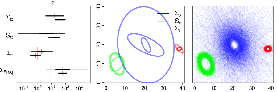
Figure 1: Simulation for two distinct sample size pairs, $n_{\alpha}=5,n_{\epsilon}=3$, and $n_{\alpha}=8,n_{\epsilon}=5$. In both, batch ${\boldsymbol{\alpha}}$ varies greater than the errors, with ${\textbf{{s}}}_{\alpha}=(\sqrt{2},\sqrt{2},\sqrt{3})^{T}$. Uncertainty intervals with thin narrow lines denoting $95\%$ uncertainty level endpoints, thicker middle portion denoting $50\%$ endpoints, and vertical tick at median. Larger red vertical ticks denote true parameter values. Higher-positioned, wider intervals correspond to smaller batch sample sizes, while lower-positioned, narrower intervals correspond to larger batch sample sizes (left). For second set of sample size pairs, ellipses from first two principal components are displayed for $2.5\%,50\%,$ and $97.5\%$ determinant-ordered percentiles of posterior distributions when $1000$ posterior realizations have been drawn (center). All $1000$ posterior ellipses (right).

For comparison, consider a frequentist approach to a simplified form of the problem. Beginning with ${\mathbf{X}}_{i}\sim{\cal{N}}_{d}({\mathbf{0}},{\boldsymbol{\Sigma}}{}),i=1,\dots,n$, it is known that ${\mathbf{U}}=\sum_{i}({\mathbf{X}}_{i}-\bar{{\mathbf{X}}})({\mathbf{X}}_{i}-\bar{{\mathbf{X}}})^{T}\sim W_{d}({\boldsymbol{\Sigma}}{},n-1)$, from which we derive the distributions

$$|{\mathbf{U}}| \sim|{\boldsymbol{\Sigma}}{}|\cdot\prod_{i=1}^{d}\chi^{2}_{n-1-d+i},$$

$${\mathbf{1}}^{T}{\mathbf{U}}{\mathbf{1}} \sim{\mathbf{1}}^{T}{\boldsymbol{\Sigma}}{}{\mathbf{1}}\cdot\chi^{2}_{n-1},$$

$$\mathrm{tr}({\mathbf{U}}) \sim\sum_{i=1}^{d}\lambda_{i}\cdot\chi^{2}_{n-1},\qquad\lambda_{1},\dots,\lambda_{d}=\textrm{eig}({\boldsymbol{\Sigma}}{}).$$

The first two offer pivots and thus allow for closed form expressions that yield confidence intervals for values of interest $|{\boldsymbol{\Sigma}}{}|,{\mathbf{1}}^{T}{\boldsymbol{\Sigma}}{}{\mathbf{1}}$. The confidence interval for $\mathrm{tr}({\boldsymbol{\Sigma}}{})$ is based on the normal approximation that matches the first two moments, $\operatorname{E}\{\mathrm{tr}({\mathbf{U}})\}=(n-1)\mathrm{tr}({\boldsymbol{\Sigma}}{})$, and $\operatorname{Var}\{\mathrm{tr}({\mathbf{U}})\}=2(n-1)\mathrm{tr}({\boldsymbol{\Sigma}}{}^{2})$. This approximation has been chosen in the spirit of moment matching approximations used by Imhof, (1961) as applied to quadratic forms of random vectors. Note that these confidence intervals assume that the ${\boldsymbol{\alpha}}_{i}$ are directly observed, which is not the case for our proposed method. Rather, the classical methods shown are included only for comparison.

To gain insight into the coverage success and uncertainty interval widths, we have carried out $S=100$ simulations over different values of $n_{\alpha}$ and each of the different scenarios of variability sources. For all simulations the number of replicates at each level is fixed at $n_{\epsilon}=15$. Results in all $3$ cases were relatively similar with respect to coverage, noting however that uncertainty interval widths increase as the magnitude of variability increases. Thus, only the scenario in which variability sources are comparable (case 3) has been shown (Figure 2). Coverage and interval widths for ${\boldsymbol{\Sigma}}{}_{\alpha}$ and ${\boldsymbol{\Sigma}}{}_{\mathrm{Freq}}$ should be compared as they correspond to the same true, unknown covariance. Despite the fact that the methodology does not assume realizations of ${\boldsymbol{\alpha}}$ to be observed directly, but rather indirectly through ${\mathbf{Y}}$, results are comparable to the frequentist approach outlined.

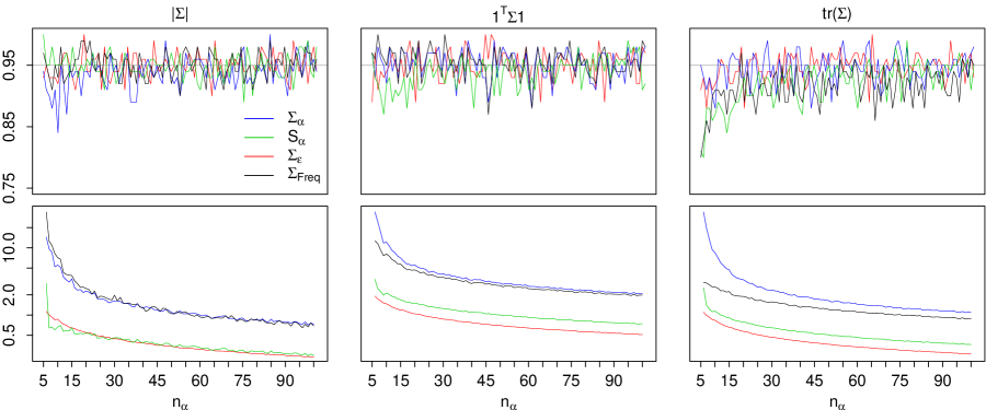
Figure 2: For $n_{\alpha}=5,\dots,100$, coverage is estimated with $S=100$ simulations in which the sources of variability are comparable (case 3). Coverage estimates for ${\boldsymbol{\Sigma}}{}_{\alpha}$, ${\mathbf{S}}_{\alpha}$, and ${\boldsymbol{\Sigma}}{}_{\epsilon}$, where grey line denotes $95\%$ nominal coverage (top). Average uncertainty interval widths on log scale (bottom).

3.2 Application

In this example our methodology is applied to a bivariate dataset of global temperature (Celsius) and precipitation (mm/day) for $9$ decadal averages of boreal summer months, June, July, August, during the remaining century. The first batch in the model consists of $13$ levels, each representing a single atmosphere-ocean general circulation model (AOGCM) developed by several international climate research institutions as part of the CMIP3 project (Meehl et al.,, 2000) in the framework of the Fourth Assessment Report (AR4) for the Intergovernmental Panel on Climate Change (IPCC). The second batch covers $3$ greenhouse gas emissions scenarios that have been defined by the Special Report on Emissions Scenarios (SRES), which are identified as A1B, A2, and B1 (Nakićenović and Swart,, 2000). One fundamental objective of the analysis is then to compare how these factors contribute to overall variability of global climate averages, how they relate to one another, and what the uncertainty of this assessment is.

Bias and dependence among climate models is an issue that has more recently begun to be examined further, beginning with Tebaldi and Knutti, (2007), Jun et al., (2008), Knutti et al., (2010), and references therein. Despite this, we adopt the statistical assumption that has traditionally been used when with working with sets of AOGCMs, which is to assume that they are independently drawn from a common process representative of true climate characteristics. Using this assumption our approach can be seen as a useful exploratory tool, and may be further adopted to address contrasts of batch levels, and thus to identify similar batch levels. Preliminary analysis steps have suggested the model

$${\mathbf{Y}}_{ijt}={\boldsymbol{\mu}}_{0}+{\boldsymbol{\alpha}}_{0,i}+{\boldsymbol{\beta}}_{0,j}+{\boldsymbol{\gamma}}_{ij}+x_{1,t}{\boldsymbol{\mu}}_{1}+x_{1,t}{\boldsymbol{\alpha}}_{1,i}+x_{1,t}{\boldsymbol{\beta}}_{1,j}+x_{2,t}{\boldsymbol{\mu}}_{2}+{\boldsymbol{\epsilon}}_{ijt},$$ (16)

where $i=1,\dots,n_{\alpha}=13$, $j=1,\dots,n_{\beta}=3$, $t=1,\dots,n_{t}=9$, $n=n_{\alpha}n_{\beta}n_{t}$, and $d=2$. Time covariate $x_{1}$ is centered such that $x_{1,t}=-4,\dots,4$, and $x_{2}$ is transformed to be orthogonal to other predictors in the model. Batches of interest are AOGCM, ${\boldsymbol{\alpha}}$, and SRES, ${\boldsymbol{\beta}}$, and their interaction, ${\boldsymbol{\gamma}}$. The first two are further specified as a constant effect, ${\boldsymbol{\alpha}}_{0},{\boldsymbol{\beta}}_{0}$, as well as with respect to time, ${\boldsymbol{\alpha}}_{1},{\boldsymbol{\beta}}_{1}$.

Posterior distributions of batches ${\boldsymbol{\alpha}}_{0},{\boldsymbol{\beta}}_{0}$, and ${\boldsymbol{\gamma}}$ are derived from (14) and (15). Batches ${\boldsymbol{\alpha}}_{1}$ and ${\boldsymbol{\beta}}_{1}$ differ slightly as they correspond to the regression model formulation. Multivariate batch levels associated with a covariate would, in general, be multiplied by a matrix, e.g. ${\mathbf{X}}_{1,t}$. Using a matrix covariate, superpopulation and batch level posteriors of batch ${\boldsymbol{\alpha}}_{1}$ are then

$${\boldsymbol{\Sigma}}{}_{\alpha_{1}}+{\mathbf{V}}_{\alpha_{1}}\mid{\mathbf{Y}},{\boldsymbol{\Sigma}}{}_{\epsilon} \sim W^{-1}\left(\sum_{i=c_{\alpha_{1}}+1}^{n_{\alpha}}\widehat{{\boldsymbol{\alpha}}}_{1,i}\widehat{{\boldsymbol{\alpha}}}_{1,i}^{T},\;n_{\alpha}-c_{\alpha_{1}}\right),$$ (17)

$${\boldsymbol{\alpha}}_{1,i}\mid{\mathbf{Y}},{\boldsymbol{\Sigma}}{}_{\epsilon},{\boldsymbol{\Sigma}}{}_{\alpha_{1}} \sim\begin{cases}{\cal{N}}_{d}\left(\widehat{{\boldsymbol{\alpha}}}_{1,i},\;\frac{n_{b}}{n}{\boldsymbol{\Sigma}}{}_{\epsilon}\right)\qquad&i=1,\dots,c_{\alpha_{1}},\\ {\cal{N}}_{d}\left({\mathbf{P}}^{-1}_{\alpha_{1}}{\textbf{{m}}}_{\alpha_{1},i},\;{\mathbf{P}}^{-1}_{\alpha_{1}}\right)\qquad&i=c_{\alpha_{1}}+1,\dots,n_{\alpha},\end{cases}$$ (18)

where ${\mathbf{V}}_{\alpha_{1}}=\frac{1}{n_{\beta}}(\sum_{t=1}^{n_{t}}{\mathbf{X}}_{1,t}^{T}{\boldsymbol{\Sigma}}{}_{\epsilon}^{-1}{\mathbf{X}}_{1,t})^{-1}$, ${\mathbf{P}}_{\alpha_{1}}={\boldsymbol{\Sigma}}{}_{\alpha_{1}}^{-1}+{\mathbf{V}}_{\alpha_{1}}^{-1}$, and ${\textbf{{m}}}_{\alpha_{1},i}={\mathbf{V}}_{\alpha_{1}}^{-1}\widehat{{\boldsymbol{\alpha}}}_{1,i}$. For model (16) the covariate matrix is ${\mathbf{X}}_{1,t}=\operatorname{diag}(x_{1,t})$, and thus ${\mathbf{V}}_{\alpha_{1}}=(n_{\beta}\sum_{t=1}^{n_{t}}x_{1,t}^{2})^{-1}{\boldsymbol{\Sigma}}{}_{\epsilon}$. The posterior of batch ${\boldsymbol{\beta}}_{1}$ is found similarly.

Figure 3 suggests that AOGCM is the most distinguishing feature. Figures 4 and 5 confirm this assessment since ${\boldsymbol{\alpha}}_{0}$ is seen as the most significant source of variability among all batches. Comparison of Figures 4, 5 also illustrate the additional uncertainty of superpopulation parameters over their finite-population counterparts. Superpopulation covariance criteria uncertainty intervals are wide because they account for uncertainty in unobserved batch levels, particularly in the case when a small number of batch levels have been observed. Finite-population covariance uncertainty intervals are generally smaller, because they are concerned with variability of only the batch levels that have been realized.

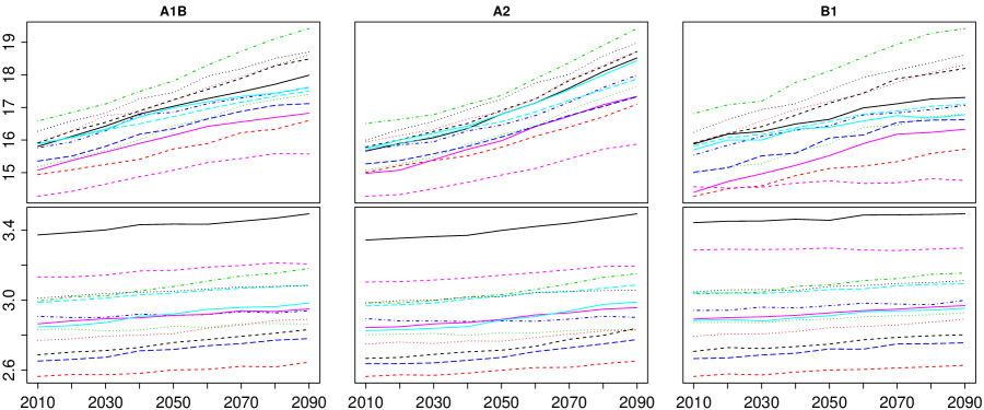
Figure 3: Global temperature (top) in degrees Celsius and precipitation (bottom) as mm/day over $n_{t}=9$ decadal intervals for $n_{\alpha}=13$ AOGCMs and $n_{\beta}=3$ emissions scenarios.

Figure 4: Superpopulation covariance uncertainty intervals using determinant, total variance, and total marginal variance criteria shown on a log scale. Nominal coverages of $0.95$ (thin lines) and $0.50$ (thick lines), and the median (vertical line) are denoted using quantiles of the corresponding posterior distributions.

Figure 5: Finite-population covariance uncertainty intervals using determinant, total variance, and total marginal variance criteria shown on a log scale. Nominal coverages of $0.95$ (thin lines) and $0.50$ (thick lines), and the median (vertical line) are denoted using quantiles of the corresponding posterior distributions.

Posterior predictive distributions, often used to perform model checking and diagnostics, can also be utilized to identify distinct sources of variability. The posterior predictive is conditional on observations with levels from each batch assumed to be, a) the same as those batch levels that have been observed data, b) unobserved/novel batch level realizations. Figure 6 examines posterior density $p(\widetilde{{\mathbf{Y}}}_{ijn_{t}}-\widetilde{{\mathbf{Y}}}_{ij1}|\{{\mathbf{Y}}_{ijt}\})$, the difference between posterior predictive distributions at the final, $t=n_{t}$, and initial, $t=1$, decades. Thus, the focus is on temporal batches, ${\boldsymbol{\alpha}}_{1i^{\prime}}$, ${\boldsymbol{\beta}}_{1j^{\prime}}$. Indices $i^{\prime},j^{\prime}$ signify new, unobserved batch levels. Linear and quadratic terms, ${\boldsymbol{\mu}}_{1},{\boldsymbol{\mu}}_{2}$ are included, although additional variability from these terms has been disregarded. The left-most panel, in which every batch contributes a new batch level realization, shows a large degree of variation. The center panel assumes that the AOGCM observed in the original data is to be used, thus variability from these specific batch level posteriors is included. For SRES a novel batch level is assumed, thus a realization utilizing the SRES superpopulation posteriors is included. A subset of three observed AOGCM levels has been displayed, selected so as to best represent the range and relative distances of their peaks. However, the high degree of variation introduced by the new emissions scenario level makes even these distributions nearly indistinguishable. In the right-most plot, using observed emissions batch levels, $n_{\beta}=3$, the additional variability introduced comes primarily from the new AOGCM batch level to be observed. The posterior predictive plots are particularly useful for determining whether the variability from each batch is due to the magnitude of the batch variability itself, or due to uncertainty in the assessment itself.

Figure 6: Posterior predictive distribution, $p({\mathbf{Y}}_{i^{\prime}j^{\prime}n_{t}}-{\mathbf{Y}}_{i^{\prime}j^{\prime}1}|\{{\mathbf{Y}}_{ijt}\})$, where both $i^{\prime},j^{\prime}$ represent new, unobserved AOGCM and SRES batch levels (left). Posterior predictive $p({\mathbf{Y}}_{ij^{\prime}n_{t}}-{\mathbf{Y}}_{ij^{\prime}1}|\{{\mathbf{Y}}_{ijt}\})$ with observed AOGCM batch levels, $i=3,9,12$ (solid, dashed, dotted) and unobserved SRES batch level ${\boldsymbol{\beta}}_{1,j^{\prime}}$ (center). Posterior predictive $p({\mathbf{Y}}_{i^{\prime}jn_{t}}-{\mathbf{Y}}_{i^{\prime}j1}|\{{\mathbf{Y}}_{ijt}\})$ with unobserved AOGCM batch level ${\boldsymbol{\alpha}}_{1,i^{\prime}}$ and all SRES levels, $j=1,2,3$ (solid, dashed, dotted), that have been observed (right). Density contours correspond to quantiles $0.05,0.25,0.75$. Horizontal and vertical axes denote precipitation in mm/day and temperature in degrees Celsius, respectively.

4 Discussion

The first contribution of this paper has been in extending recent philosophical shifts in the treatment of analysis of variance to multivariate settings. New analysis of variance approaches allow appropriate parameters, e.g. super or finite population, to be used to answer the correct research question, while at the same time providing coherent model definition, implementation, and interpretation. This same flexibility has been extended to multivariate cases; in that the researcher can guide covariance criteria choices, rather than the method determining the criterion. The second contribution has been in providing a foundation for computational efficiency, which is necessary for dimension scalability. Using improper batch level priors we have shown that it is possible to minimize dependencies between batch covariances. In many cases this reduces, or eliminates, the need for complex and computationally demanding analyses.

Further extensions to the methodology must explicitly address increasing dimensionality. For moderately sized dimensions $d$, relative to number of observations, improper inverse-Wishart distributions, and/or priors that impose particular dependence structures, are possible options. For cases in which $d$ is very large, stricter covariance assumptions may be employed. In the spatial context, properties such as stationarity allow covariance parameter space to be reduced, e.g. range, sill, and nugget in a spatial covariance function. Because simultaneous estimation of such parameters is nontrivial, some parameters are often assumed, or estimated empirically in earlier analysis steps, as in Furrer et al., (2007). In other cases, so as to maintain computational feasibility, sparsity restrictions are placed on covariances (Cressie and Johannesson,, 2008; Furrer et al.,, 2006; Stein,, 2008). For many such scenarios a covariance is decomposed into a correlation matrix and a scalar variance parameter. Our method is then carried out with the inverse-Wishart posterior density transformed through a spectral decomposition of the correlation matrix, thus allowing for efficient posterior sampling for cases in which $d\gg n$. This extension offers an alternative to geostatistical model analyses that have previously relied on computationally intensive MCMC methods, and is the focus of current research. Other difficulties encountered are unbalanced designs and linearly dependent predictors. MCMC may be utilized for sets of dependent batch levels. Development for these cases is another area of current research.

Acknowledgments
We acknowledge the modeling groups, the Program for Climate Model Diagnosis and Intercomparison (PCMDI) and the WCRP’s Working Group on Coupled Modeling (WGCM) for their roles in making available the WCRP CMIP3 multi-model dataset. Support of this dataset is provided by the Office of Science, U.S. Department of Energy.

References

- Cressie and Johannesson, (2008) Cressie, N. and Johannesson, G. (2008). Fixed rank kriging for very large spatial data sets. J. R. Stat. Soc. Ser. B Stat. Methodol., 70, 209–226.
- Daniels, (1999) Daniels, M. J. (1999). A prior for the variance in hierarchical models. Canad. J. Statist., 27, 567–578.
- Daniels and Kass, (2001) Daniels, M. J. and Kass, R. E. (2001). Shrinkage estimators for covariance matrices. Biometrics, 57, 1173–1184.
- Díaz-García et al., (1997) Díaz-García, J. A., Gutierrez Jáimez, R., and Mardia, K. V. (1997). Wishart and pseudo-Wishart distributions and some applications to shape theory. J. Multivariate Anal., 63, 73–87.
- Everson and Morris, (2000) Everson, P. J. and Morris, C. N. (2000). Simulation from Wishart distributions with eigenvalue constraints. J. Comput. Graph. Statist., 9, 380–389.
- Furrer et al., (2006) Furrer, R., Genton, M. G., and Nychka, D. (2006). Covariance tapering for interpolation of large spatial datasets. J. Comput. Graph. Statist., 15, 502–523.
- Furrer et al., (2007) Furrer, R., Sain, S. R., Nychka, D. W., and Meehl, G. A. (2007). Multivariate Bayesian analysis of atmosphere-ocean general circulation models. Environ. Ecol. Stat., 14, 249–266.
- Gelman, (2005) Gelman, A. (2005). Analysis of variance: Why it is more important than ever. Ann. Statist., 33, 1–31.
- Gelman and Hill, (2006) Gelman, A. and Hill, J. (2006). Data Analysis Using Regression and Multilevel/Hierarchical Models. Cambridge University Press, 1st edition.
- Imhof, (1961) Imhof, J. P. (1961). Computing the distribution of quadratic forms in normal variables. Biometrika, 48, 419–426.
- Jun et al., (2008) Jun, M., Knutti, R., and Nychka, D. W. (2008). Spatial analysis to quantify numerical model bias and dependence: How many climate models are there? J. Amer. Statist. Assoc., 103, 934–947.
- Kaufman and Sain, (2010) Kaufman, C. G. and Sain, S. R. (2010). Bayesian functional ANOVA modeling using Gaussian process prior distributions. Bayesian Anal., 5, 847–874.
- Knutti et al., (2010) Knutti, R., Furrer, R., Tebaldi, C., Cermak, J., and Meehl, G. A. (2010). Challenges in combining projections from multiple climate models. Journal of Climate, 23, 2739–2758.
- Leinonen et al., (2008) Leinonen, T., O’Hara, R. B., Cano, J. M., and Merilä, J. (2008). Comparative studies of quantitative trait and neutral marker divergence: a meta-analysis. Journal of Evolutionary Biology, 21, 1–17.
- Lencina et al., (2005) Lencina, V. B., Singer, J. M., and Stanek, E. J. (2005). Much ado about nothing: the mixed models controversy revisited. International Statistical Review, 73, 9–20.
- Lindgren et al., (2011) Lindgren, F., Rue, H., and Lindström, J. (2011). An explicit link between gaussian fields and gaussian markov random fields: the stochastic partial differential equation approach. J. R. Stat. Soc. Ser. B Stat. Methodol., 73, 423–498.
- Mardia et al., (1979) Mardia, K. V., Kent, J. T., and Bibby, J. M. (1979). Multivariate Analysis. Academic Press.
- Meehl et al., (2000) Meehl, G. A., Boer, G. J., Covey, C., Latif, M., and Stouffer, R. J. (2000). The coupled model intercomparison project (CMIP). American Meteorological Society Bulletin, 81, 313–318.
- Nakićenović and Swart, (2000) Nakićenović, N. and Swart, R., editors (2000). Special Report on Emission Scenarios. Intergovernmental Panel on Climate Change, Cambridge University Press.
- Nelder, (1977) Nelder, J. A. (1977). A reformulation of linear models. J. Roy. Statist. Soc. Ser. A, 140, 48–77.
- Nelder, (1994) Nelder, J. A. (1994). The statistics of linear models: back to basics. Statist. Comput., 4, 221–234.
- Nelder, (1999) Nelder, J. A. (1999). From statistics to statistical science. J. R. Stat. Soc. Ser. D The Statistician, 48, 257–269.
- Nelder, (2008) Nelder, J. A. (2008). What is the mixed-models controversy? International Statistical Review, 76, 134–135.
- Qian and Shen, (2007) Qian, S. S. and Shen, Z. (2007). Ecological applications of multilevel analysis of variance. Ecology, 88, 2489–2495.
- Rue and Held, (2005) Rue, H. and Held, L. (2005). Gaussian Markov Random Fields: Theory and Applications. Chapman & Hall, London.
- Rue et al., (2009) Rue, H., Martino, S., and Chopin, N. (2009). Approximate Bayesian inference for latent gaussian models by using integrated nested laplace approximations. J. R. Stat. Soc. Ser. B Stat. Methodol., 71, 1–35.
- Sain et al., (2011) Sain, S. R., Nychka, D., and Mearns, L. (2011). Functional ANOVA and regional climate experiments: a statistical analysis of dynamic downscaling. Environmetrics, 22, 700–711.
- Srivastava, (2003) Srivastava, M. S. (2003). Singular Wishart and multivariate beta distributions. Ann. Statist., 31, 1537–1560.
- Stein, (2008) Stein, M. L. (2008). A modeling approach for large spatial datasets. J. Korean Statist. Soc., 37, 3–10.
- Tebaldi and Knutti, (2007) Tebaldi, C. and Knutti, R. (2007). The use of the multi-model ensemble in probabilistic climate projections. Philos. Trans. R. Soc. Lond. Ser. A Math. Phys. Eng. Sci., 365, 2053–2075.
- Uhlig, (1994) Uhlig, H. (1994). On singular Wishart and singular multivariate beta distributions. Ann. Statist., 22, 395–405.
- Voss, (1999) Voss, D. T. (1999). Resolving the mixed models controversy. Amer. Statist., 53, 352–356.