SHO-FA: Robust compressive sensing with order-optimal complexity, measurements, and bits

Abstract

Suppose ${\mathbf{x}}$ is any exactly ${k}$-sparse vector in ⁿ. We present a class of “sparse” matrices ${{A}}$, and a corresponding algorithm that we call SHO-FA (for Short and Fast) that, with high probability over ${{A}}$, can reconstruct ${\mathbf{x}}$ from ${{A}}{\mathbf{x}}$. The SHO-FA algorithm is related to the Invertible Bloom Lookup Tables (IBLTs) recently introduced by Goodrich et al., with two important distinctions – SHO-FA relies on linear measurements, and is robust to noise. The SHO-FA algorithm is the first to simultaneously have the following properties: (a) it requires only ${\mathcal{O}}({k})$ measurements, (b) the bit-precision of each measurement and each arithmetic operation is ${\mathcal{O}}\left(\log({n})+P\right)$ (here $2^{-P}$ corresponds to the desired relative error in the reconstruction of ${\mathbf{x}}$), (c) the computational complexity of decoding is ${\mathcal{O}}({k})$ arithmetic operations and that of encoding is ${\mathcal{O}}({n})$ arithmetic operations, and (d) if the reconstruction goal is simply to recover a single component of ${\mathbf{x}}$ instead of all of ${\mathbf{x}}$, with significant probability over ${{A}}$ this can be done in constant time. All constants above are independent of all problem parameters other than the desired probability of success. For a wide range of parameters these properties are information-theoretically order-optimal. In addition, our SHO-FA algorithm works over fairly general ensembles of “sparse random matrices”, is robust to random noise, and (random) approximate sparsity for a large range of ${k}$. In particular, suppose the measured vector equals ${{A}}({\mathbf{x}}+{\mathbf{z}})+{\mathbf{e}}$, where ${\mathbf{z}}$ and ${\mathbf{e}}$ correspond respectively to the source tail and measurement noise. Under reasonable statistical assumptions on ${\mathbf{z}}$ and ${\mathbf{e}}$ our decoding algorithm reconstructs ${\mathbf{x}}$ with an estimation error of ${\mathcal{O}}(||{\mathbf{z}}||_{2}+||{\mathbf{e}}||_{2})$. The SHO-FA algorithm works with high probability over ${{A}}$, ${\mathbf{z}}$, and ${\mathbf{e}}$, and still requires only ${\mathcal{O}}({k})$ steps and ${\mathcal{O}}({k})$ measurements over ${\mathcal{O}}(\log({n}))$-bit numbers. This is in contrast to most existing algorithms which focus on the “worst-case” ${\mathbf{z}}$ model, where it is known $\Omega({k}\log({n}/{k}))$ measurements over ${\mathcal{O}}(\log({n}))$-bit numbers are necessary. Our algorithm has good empirical performance, as validated by simulations.

I Introduction

In recent years, spurred by the seminal work on compressive sensing of [3, 4], much attention has focused on the problem of reconstructing a length-${n}$ “compressible” vector ${\mathbf{x}}$ over with fewer than ${n}$ linear measurements. In particular, it is known (e.g. [5, 6]) that with ${m}={\mathcal{O}}({k}\log({n}/{k}))$ linear measurements one can computationally efficiently obtain a vector ${\hat{{\mathbf{x}}}}$ such that the reconstruction error $||{\mathbf{x}}-{\hat{{\mathbf{x}}}}||_{1}$ is ${\mathcal{O}}(||{\mathbf{x}}-{{{\mathbf{x}}_{{k}}}^{\ast}}||_{1})$, where ${{{\mathbf{x}}_{{k}}}^{\ast}}$ is the best possible ${k}$-sparse approximation to ${\mathbf{x}}$ (specifically, the ${k}$ non-zero terms of ${{{\mathbf{x}}_{{k}}}^{\ast}}$ correspond to the ${k}$ largest components of ${\mathbf{x}}$ in magnitude, hence ${\mathbf{x}}-{{{\mathbf{x}}_{{k}}}^{\ast}}$ corresponds to the “tail” of ${\mathbf{x}}$). A number of different classes of algorithms are able to give such performance, such as those based on ${\mathscr{l}}_{1}$-optimization (e.g. [3, 4]), and those based on iterative “matching pursuit” (e.g. [10, 11]). Similar results, with an additional additive term in the reconstruction error hold even if the linear measurements themselves also have noise added to them (e.g. [5, 6]). The fastest of these algorithms use ideas from the theory of expander graphs, and have running time ${\mathcal{O}}({n}\log({n}/{k}))$ [12, 13, 14].

The class of results summarized above are indeed very strong – they hold for all ${\mathbf{x}}$ vectors, including those with “worst-case tails”, i.e. even vectors where the components of ${\mathbf{x}}$ smaller than the ${k}$ largest coefficients (which can be thought of as “source tail”) are chosen in a maximally worst-case manner. In fact [15] proves that to obtain a reconstruction error that scales linearly with the ${\mathscr{l}}_{1}$-norm of the ${\mathbf{z}}$, the tail of ${\mathbf{x}}$, requires $\Omega({k}\log({n}/{k}))$ linear measurements.

Number of measurements: However, depending on the application, such a lower bound based on “worst-case ${\mathbf{z}}$” may be unduly pessimistic. For instance, it is known that if ${\mathbf{x}}$ is exactly ${k}$-sparse (has exactly exactly ${k}$ non-zero components, and hence ${\mathbf{z}}=\mathbf{0}$), then based on Reed-Solomon codes [16] one can efficiently reconstruct ${\mathbf{x}}$ with ${\mathcal{O}}({k})$ noiseless measurements (e.g. [17]) via algorithms with decoding time-complexity ${\mathcal{O}}({n}\log({n}))$, or via codes such as in [18, 19] with ${\mathcal{O}}({k})$ noiseless measurements with decoding time-complexity ${\mathcal{O}}({n})$. In the regime where ${k}=\theta({n})$ [20] use the “sparse-matrix” techniques of [12, 13, 14] to demonstrate that ${\mathcal{O}}({k})={\mathcal{O}}({n})$ measurements suffice to reconstruct ${\mathbf{x}}$.

Noise: Even if the source is not exactly ${k}$-sparse, a spate of recent work has taken a more information-theoretic view than the coding-theoretic/worst-case point-of-view espoused by much of the compressive sensing work thus far. Specifically, suppose the length-${n}$ source vector is the sum of any exactly ${k}$-sparse vector ${\mathbf{x}}$ and a “random” source noise vector ${\mathbf{z}}$ (and possibly the linear measurement vector ${{A}}({\mathbf{x}}+{\mathbf{z}})$ also has a “random” measurement noise vector ${\mathbf{e}}$ added to it). Then as long as the noise variances are not “too much larger” than the signal power, the work of [21] demonstrates that ${\mathcal{O}}({k})$ measurements suffice (though the proofs in [21] are information-theoretic and existential – the corresponding “typical-set decoding” algorithms require time exponential in ${n}$). Indeed, even the work of [15], whose primary focus was to prove that $\Omega({k}\log({n}/{k}))$ linear measurements are necessary to reconstruct ${\mathbf{x}}$ in the worst case, also notes as an aside that if ${\mathbf{x}}$ corresponds to an exactly sparse vector plus random noise, then in fact ${\mathcal{O}}({k})$ measurements suffice. The work in [22, 23] examines this phenomenon information-theoretically by drawing a nice connection with the Rényi information dimension $\bar{d}(X)$ of the signal/noise. The heuristic algorithms in [24] indicate that approximate message passing algorithms achieve this performance computationally efficiently (in time ${\mathcal{O}}({n}^{2})$), and [25] prove this rigorously. Corresponding lower bounds showing $\Omega({k}\log({n}/{k}))$ samples are required in the higher noise regime are provided in [26, 27].

Number of measurement bits: However, most of the works above focus on minimizing the number of linear measurements in ${{A}}{\mathbf{x}}$, rather than the more information-theoretic view of trying to minimize the number of bits in ${{A}}{\mathbf{x}}$ over all measurements. Some recent work attempts to fill this gap – notably “Counting Braids” [28, 29] (this work uses “multi-layered non-linear measurements”), and “one-bit compressive sensing” [30, 31] (the corresponding decoding complexity is somewhat high (though still polynomial-time) since it involves solving an LP).

Decoding time-complexity: The emphasis of the discussion thus far has been on the number of linear measurements/bits required to reconstruct ${\mathbf{x}}$. The decoding algorithms in most of the works above have decoding time-complexities that scale at least linearly with ${n}$. In regimes where ${k}$ is significantly smaller than ${n}$, it is natural to wonder whether one can do better. Indeed, algorithms based on iterative techniques answer this in the affirmative. These include Chaining Pursuit [32], group-testing based algorithms [33], and Sudocodes [34] – each of these have decoding time-complexity that can be sub-linear in ${n}$ (but at least ${\mathcal{O}}({k}\log({k})\log({n}))$), but each requires at least ${\mathcal{O}}({k}\log({n}))$ linear measurements.

Database query: Finally, we consider a database query property that is not often of primary concern in the compressive sensing literature. That is, suppose one is given a compressive sensing algorithm that is capable of reconstructing ${\mathbf{x}}$ with the desired reconstruction guarantee. Now suppose that one instead wishes to reconstruct, with reasonably high probability, just “a few” (constant number) specific components of ${\mathbf{x}}$, rather than all of it. Is it possible to do so even faster (say in constant time) – for instance, if the measurements are in a database, and one wishes to query it in a computationally efficient manner? If the matrix ${{A}}$ is “dense” (most of its entries are non-zero) then one can directly see that this is impossible. However, several compressive sensing algorithms (for instance [20]) are based on “sparse” matrices ${{A}}$, and it can be shown that in fact these algorithms do indeed have this property “for free” (as indeed does our algorithm), even though the authors do not analyze this. As can be inferred from the name, this database query property is more often considered in the database community, for instance in the work on IBLTs [35].

I-A Our contributions

Conceptually, the “iterative decoding” technique we use is not new. Similar ideas have been used in various settings in, for instance  [36, 37, 35, 18]. However, to the best of our knowledge, no prior work has the same performance as our work – namely – information-theoretically order-optimal number of measurements, bits in those measurements, and time-complexity, for the problem of reconstructing a sparse signal (or sparse signal with a noisy tail and noisy measurements) via linear measurements (along with the database query property).The key to this performance is our novel design of “sparse random” linear measurements, as described in Section II.

To summarize, the desirable properties of SHO-FA are that with high probability:

• Number of measurements: For every ${k}$-sparse ${\mathbf{x}}$, with high probability over ${{A}}$, ${\mathcal{O}}({k})$ linear measurements suffice to reconstruct ${\mathbf{x}}$. This is information-theoretically order-optimal.

• Number of measurement bits: The total number of bits in ${{A}}{\mathbf{x}}$ required to reconstruct ${\mathbf{x}}$ to a relative error of $2^{-P}$ is ${\mathcal{O}}({k}(\log({n})+P))$. This is information-theoretically order-optimal for any ${k}={\mathcal{O}}({n}^{1-\Delta})$ (for any $\Delta>0$).

• Decoding time-complexity: The total number of arithmetic operations required is ${\mathcal{O}}({k})$. This is information-theoretically order-optimal.

• “Database-type queries”: With constant probability $1-\epsilon$ any single “database-type query” can be answered in constant time. That is, the value of a single component of ${\mathbf{x}}$ can be reconstructed in constant time with constant probability.

• Encoding/update complexity: The computational complexity of generating ${{A}}{\mathbf{x}}$ from ${{A}}$ and ${\mathbf{x}}$ is ${\mathcal{O}}({n})$, and if ${\mathbf{x}}$ changes to some ${\mathbf{x}}^{\prime}$ in ${\mathcal{O}}(1)$ locations, the computational complexity of updating ${{A}}{\mathbf{x}}$ to ${{A}}{\mathbf{x}}^{\prime}$ is ${\mathcal{O}}(1)$. Both of these are information-theoretically order-optimal.

• Noise: Suppose ${\mathbf{z}}$ and ${\mathbf{e}}$ have i.i.d. components drawn respectively from ${\mathcal{N}}(0,\sigma_{z}^{2})$ and ${\mathcal{N}}(0,\sigma_{e}^{2})$. For every $\epsilon^{\prime}>0$ and for ${k}={\mathcal{O}}({n}^{1-\Delta})$ for any $\Delta>0$, a modified version of SHO-FA (SHO-FA-NO) that with high probability reconstructs ${\mathbf{x}}$ with an estimation error of $(1+\epsilon^{\prime})(||{\mathbf{z}}||_{2}+||{\mathbf{e}}||_{2})$.

• Practicality: As validated by simulations (shown in Appendix -I), most of the constant factors involved above are not large.

• Different bases: As is common in the compressive sensing literature, our techniques generalize directly to the setting wherein ${\mathbf{x}}$ is sparse in an alternative basis (say, for example, in a wavelet basis).

• Universality: While we present a specific ensemble of matrices over which SHO-FA operates, we argue that in fact similar algorithms work over fairly general ensembles of “sparse random matrices” (see Section IV), and further that such matrices can occur in applications, for instance in wireless MIMO systems [40] (Figure 10 gives such an example) and Network Tomography [41].

Figure 1: A comparison of prior work with this work (and that of [2]) in two parameters – decoding complexity, and number of measurements. Information-theoretic bounds show that the shaded region is infeasible. Only some of the many prior results in the field of Compressive Sensing are plotted here (some other works are referenced in the following table). Since ${k}$ and ${n}$ do not scale together in a fixed manner, the position of points in this graph should be interpreted in a relative rather than absolute manner. The constants $\alpha$ and $\beta$ are intended to represent the degrees of “small” polynomials.

Reference	${{A}}$	${\mathbf{x}}$	${\mathbf{z}}$	${\mathbf{e}}$	Reconstruction	$\mathbf{P_{e}}$	# Measurements	# Decoding steps	Precision
					Goal
Reed-Solomon [16]	D	D	$0$	$0$	Exact	$0$	$2{k}+1$	${\mathcal{O}}({n}\log{n}))$ [42]	–
Singleton [43]	D/R	D	$0$	$0$	Exact	$0$	$\geq 2{k}$	–	–
Mitzenmacher-Varghese [19]	R	D	$0$	$0$	Exact	${\mathcal{O}}(1)$	${\mathcal{O}}({k})$	${\mathcal{O}}({n})$	–
Kudekar-Pfister [18]	R	D	$0$	$0$	Exact	$o(1)$	${\mathcal{O}}({k})$	${\mathcal{O}}({n})$	–
Tropp-Gilbert [10]	G	D	$0$	$0$	Exact	$o(1)$	${\mathcal{O}}({k}\log({n}))$	${\mathcal{O}}({k}^{2}{n}\log({n}))$	–
Wu-Verdú ’10 [22]	R	R	R	$0$	Exact	$o(1)$	${n}\bar{d}({\mathbf{x}}+{\mathbf{z}})+o({n})$	${\mathcal{O}}(\exp({n}))$	–
Donoho et al. [25]	R	R	R	$0$	Exact	o(1)	${n}\bar{d}({\mathbf{x}}+{\mathbf{z}})+o({n})$	${\mathcal{O}}({n}^{3})$	–
				R	${\mathscr{l}}_{2}<{C}{\mathscr{l}}_{2}$
Cormode-Muthukrishnan  [33]	R	D	$0$	$0$	${\mathscr{l}}_{2}<{C}{\mathscr{l}}_{2}$	$o(1)$	${\mathcal{O}}({k}\;\mbox{poly}(\log({n})))$	${\mathcal{O}}({k}\;\mbox{poly}(\log({n})))$	–
Cohen et al. [7]	D	D	D	$0$	${\mathscr{l}}_{2}<{C}{\mathscr{l}}_{2}$	$0$	$\Omega({n})$	–	–
Price-Woodruff [9]	D	D	D	$0$	${\mathscr{l}}_{2}<{C}{\mathscr{l}}_{2}$	$o(1)$	$\theta({k}\log({n}/{k}))$	–	–
Ba et al. [15]	D/R	D	D	$0$	${\mathscr{l}}_{1}<{C}{\mathscr{l}}_{1}$	${\mathcal{O}}(1)$	$\Omega({k}\log({n}/{k}))$	–	${\mathcal{O}}(\log({n}))$
Ba et al. [15]	R	D	R	$0$	${\mathscr{l}}_{2}<{C}{\mathscr{l}}_{2}$	$o(1)$	${\mathcal{O}}({k})$	${\mathcal{O}}(\exp({n}))$
Candés [5],	R	D	D	D	${\mathscr{l}}_{2}<\frac{C}{\sqrt{{k}}}{\mathscr{l}}_{1}$	$o(1)$	${\mathcal{O}}({k}\log({n}/{k}))$	LP	–
Baraniuk et al. [6]
Indyk et al. [44]	D	D	D	D	${\mathscr{l}}_{1}<(1+\epsilon){\mathscr{l}}_{1}$	$0$	${\mathcal{O}}({k}\log({n}/{k}))$	${\mathcal{O}}({n}\log({n}/{k}))$	–
Akçakaya et al. [45]	R	D	$0$	R	${\mathscr{l}}_{2}<{C}{\mathscr{l}}_{2}/$	$0$	${\mathcal{O}}({k})$	${\mathcal{O}}(\exp({n}))$	–
					Sup. Rec.		Cond. on $x_{min}$
Wu-Verdú ’11 [23]	R	R	R	R	${\mathscr{l}}_{2}<{C}{\mathscr{l}}_{2}$	${\mathcal{O}}(1)$	$\bar{d}({\mathbf{x}}+{\mathbf{z}})$	${\mathcal{O}}(\exp({n}))$	–
Wainwright [27]	${\mathcal{N}}$	D	$0$	R	Sup. Rec.	${\mathcal{O}}(1)$	$\Omega({k}\log({n}/{k}))$	–	–
Fletcher et al. [26]	${\mathcal{N}}$	D	$0$	R	Sup. Rec.	$o(1)$	${\mathcal{O}}({k}\log({n}-{k}))$	–	–
Aeron et al. [46]	${\mathcal{N}}$	D	$0$	R	Sup. Rec.	${\mathcal{O}}(1)$	$\Omega({k}\log({n}/{k}))$		–
Plan-Vershynin [30]	R	D	$0$	sgn	${\mathscr{l}}_{2}<f({\mathbf{x}},{\mathbf{x}}_{{k}})$	${\mathcal{O}}(1)$	${k}^{2}\log({n}/{k})$	LP	1
Jacques et al. [31]	R	D	$0$	sgn	${\mathscr{l}}_{2}<f^{\prime}({n},{k})$	${\mathcal{O}}(1)$	${k}\log({n})$	$\exp({n})$	1
Sarvotham et al. [34]	R	D	$0$	$0$	Exact	${\mathcal{O}}(1)$	${k}\log({n})$	${k}\log({k})\log({n})$	–
Gilbert et al. [32]	R	P.L.	P.L.	0	${\mathscr{l}}_{1}<{[1+C\log({n})]}{\mathscr{l}}_{1}$	${\mathcal{O}}(1)$	${k}\log^{2}({n})$	${k}\log^{2}({n})\log^{2}({k})$	–
This work/Pawar et al. [2]	R	D	$0$	$0$	Exact	$o(1)$	${\mathcal{O}}({k})$	${\mathcal{O}}({k})$	${\mathcal{O}}(\log({n})+P)$
	R	D	R	R	${\mathscr{l}}_{1}<{C}{\mathscr{l}}_{1}$	$o(1)$	${\mathcal{O}}({k})$	${\mathcal{O}}({k})$	${\mathcal{O}}(\log({n}))$

Explanations and discussion: At the risk of missing much of the literature, and also perhaps oversimplifying nuanced results, we summarize in this table many of the strands of work preceding this paper and related to it – not all results from each work are represented in this table. The second to the fifth columns respectively reference whether the measurement matrix ${{A}}$, source ${k}$-sparse vector ${\mathbf{x}}$, source noise ${\mathbf{z}}$, and measurement noise ${\mathbf{e}}$ are random (R) or deterministic (D) – a $0$ in a column corresponding to noise indicates that that work did not consider that type of noise. An entry “P.L.” stands for “Power Law” decay in columns corresponding to ${\mathbf{x}}$ and ${\mathbf{z}}$. For achievability schemes, in general $D$-type results are stronger than $R$-type results, which in turn are stronger than $0$-type results. This is because a $D$-type result for the measurement matrix indicates that there is an explicit construction of a matrix that satisfies the required goals, whereas the $R$-type results generally indicate that the result is true with high probability over measurement matrices. Analogously, a $D$ in the columns corresponding to ${\mathbf{x}}$, ${\mathbf{z}}$ or ${\mathbf{e}}$ indicates that the scheme is true for all vectors, whereas an $R$ indicates that it is true for random vectors from some suitable ensemble. For converse results, the the opposite is true $0$ results are stronger than $R$-type results, which are stronger than $D$-type results. An entry ${\mathcal{N}}$ indicates the normal distribution – the results of [27] and [26] are converses for matrices with i.i.d. Gaussian entries. An entry “sgn” denotes (in the case of works dealing with one-bit measurements) that the errors are sign errors. The sixth column corresponds to what the desired goal is. The strongest possible goal is to have exact reconstruction of ${\mathbf{x}}$ (up to quantization error due to finite-precision artihmetic), but this is not always possible, especially in the presence of noise. Other possible goals include “Sup. Rec. ” (short for support recovery) of ${\mathbf{x}}$, or that the reconstruction $\hat{{\mathbf{x}}}$ of ${\mathbf{x}}$ differs from ${\mathbf{x}}$ as a “small” function of ${\mathbf{z}}$. It is known that if a deterministic reconstruction algorithm is desired to work for all ${\mathbf{x}}$ and ${\mathbf{z}}$, then $||\hat{{\mathbf{x}}}-{\mathbf{x}}||_{2}<{\mathcal{O}}(||{\mathbf{z}}||_{2})$ is not possible with less than $\Omega({n})$ measurements [7], and that $||\hat{{\mathbf{x}}}-{\mathbf{x}}||_{2}<{\mathcal{O}}(||{\mathbf{z}}||_{1}/\sqrt{{k}})$ implies $||\hat{{\mathbf{x}}}-{\mathbf{x}}||_{1}<{\mathcal{O}}(||{\mathbf{z}}||_{1})$. The reconstruction guarantees in [30, 31] unfortunately do not fall neatly in these categories. The seventh column indicates what the probability of error is – i.e. the probability over any randomness in ${{A}}$, ${\mathbf{x}}$, ${\mathbf{z}}$ and ${\mathbf{e}}$ that the reconstruction goal in the sixth column is not met. In the eighth column, some entries are marked $\bar{d}({\mathbf{x}}+{\mathbf{z}})$ – this denotes the (upper) Rényi dimension of ${\mathbf{x}}+{\mathbf{z}}$ – in the case of exactly ${k}$-sparse vectors this equals ${k}$, but for non-zero ${\mathbf{z}}$ it depends on the distribution of ${\mathbf{z}}$. The ninth column considers the computational complexity of the algorithms – the entry “LP” denotes the computational complexity of solving a linear program. The final column notes whether the particular work referenced considers the precision of arithmetic operations, and if so, to what level.

I-B Special acknowledgements

While writing this paper, we became aware of parallel and independent work by Pawar and Ramchandran [2] that relies on ideas similar to our work and achieves similar performance guarantees. Both the work of [2] and the preliminary version of this work [1] were presented at the same venue.

In particular, the bounds on the minimum number of measurements required for “worst-case” recovery and the corresponding discussion on recovery of signals with “random tails” in [15] led us to consider this problem in the first place. Equally, the class of compressive sensing codes in [20], which in turn build upon the constructions of expander codes in [36], have been influential in leading us to this work. While the model in [37] differs from the one in this work, the techniques therein are of significant interest in our work. The analysis in [37] of the number of disjoint components in certain classes of random graphs, and also the analysis of how noise propagates in iterative decoding is potentially useful sharpening our results. We elaborate on these in Section III.

The work that is conceptually the closest to SHO-FA is that of the Invertible Bloom Lookup Tables (IBLTs) introduced by Goodrich-Mitzenmacher [35] (though our results were derived independently, and hence much of our analysis follows a different line of reasoning). The data structures and iterative decoding procedure (called “peeling” in [35]) used are structurally very similar to the ones used in this work. However the “measurements” in IBLTs are fundamentally non-linear in nature – specifically, each measurement includes within it a “counter” variable – it is not obvious how to implement this in a linear manner. Therefore, though the underlying graphical structure of our algorithms is similar, the details of our implementation require new non-trivial ideas. Also, IBLTs as described are not robust to either signal tails or measurement noise. Nonetheless, the ideas in [35] have been influential in this work. In particular, the notion that an individual component of ${\mathbf{x}}$ could be recovered in constant time, a common feature of Bloom filters, came to our notice due to this work.

II Exactly ${k}$-sparse ${\mathbf{x}}$ and noiseless measurements

We first consider the simpler case when the source signal is exactly ${k}$-sparse and the measurements are noiseless, i.e., ${\mathbf{y}}={{A}}{\mathbf{x}}$, and both ${\mathbf{z}}$ and ${\mathbf{e}}$ are all-zero vectors. The intuition presented here carries over to the scenario wherein both ${\mathbf{z}}$ and ${\mathbf{e}}$ are non-zero, considered separately in Section III

For ${k}$-sparse input vectors ${\mathbf{x}}\in{}^{{n}}$ let the set ${\mathcal{S}}({\mathbf{x}})$ denote its support, i.e., its set of nonzero values $\{{j}:x_{{j}}\neq 0\}$. Recall that in our notation, for some ${m}$, a measurement matrix ${{A}}\in{}^{{m}\times{n}}$ is chosen probabilistically. This matrix operates on ${\mathbf{x}}$ to yield the measurement vector ${\mathbf{y}}\in{}^{{m}}$ as ${\mathbf{y}}={{A}}{\mathbf{x}}$. The decoder takes the vector ${\mathbf{y}}$ as input and outputs the reconstruction $\hat{{\mathbf{x}}}\in\mathbb{R}^{{n}}$ – it is desired that $\hat{{\mathbf{x}}}$ equal ${\mathbf{x}}$ (with upto $P$ bits of precision) with high probability over the choice of measurement matrices .

In this section, we describe a probabilistic construction of the measurement matrix ${{A}}$ and a reconstruction algorithm SHO-FA that achieves the following guarantees.

Theorem 1.

Let ${k}\leq{n}$. There exists a reconstruction algorithm SHO-FA for ${{A}}\in{}^{{m}\times{n}}$ with the following properties:

1. For every ${\mathbf{x}}\in\mathbb{R}^{{n}}$, with probability $1-{\mathcal{O}}(1/{k})$ over the choice of ${{A}}$, SHO-FA produces a reconstruction $\hat{{\mathbf{x}}}$ such that $||{\mathbf{x}}-\hat{{\mathbf{x}}}||_{1}/||{\mathbf{x}}||_{1}\leq 2^{-P}$

2. The number of measurements ${m}={c}{k}$ for some ${c}>0$

3. The number of steps required by SHO-FA is ${\mathcal{O}}({k})$

4. The number of bitwise arithmetic operations required by SHO-FA is ${\mathcal{O}}({k}(\log{{n}}+P))$.

We present a “simple” proof of the above theorem in Sections II-A to II-F. In Section II-H1 we direct the reader to an alternative, more technically challenging, analysis (based on the work of [35]) that leads to a tighter characterization of the constant factors in the parameters of Theorem 1.

II-A High-level intuition

If ${m}=\Theta({n})$, the task of reconstructing ${\mathbf{x}}$ from ${\mathbf{y}}={{A}}{\mathbf{x}}$ appears similar to that of syndrome decoding of a channel code of rate ${n}/{m}$ [47]. It is well-known [48] that channel codes based on bipartite expander graphs, i.e., bipartite graphs with good expansion guarantees for all sets of size less than or equal to ${k}$, allow for decoding in a number of steps that is linear in the size of ${\mathbf{x}}$. In particular, given such a bipartite expander graph with ${n}$ nodes on the left and ${m}$ nodes on the right, choosing the matrix ${{A}}$ as a ${m}\times{n}$ binary matrix with non-zero values in the locations where the corresponding pair of nodes in the graph has an edge is known to result in codes with rate and relative minimum distance that is linear in ${n}$.

Motivated by this [20] explore a measurement design that is derived from expander graphs and show that ${\mathcal{O}}({k}\log({n}/{k}))$ measurements suffice, and ${\mathcal{O}}({k})$ iterations with overall decoding complexity of ${\mathcal{O}}({n}\log{({n}/{k})})$.

It is tempting to think that perhaps an optimized application of expander graphs could result in a design that require only ${\mathcal{O}}({k})$ number of measurements. However, we show that in the compressive sensing setting, where, typically ${k}=o({n})$, it is not possible to satisfy the desired expansion properties. In particular, if one tries to mimic the approach of [20], one would need bipartite expanders such that all sets of size ${k}$ on one side of the graph “expand” – we show in Lemma 2 that this is not possible. As such, this result may be of independent interest for other work that require similar graphical constructions (for instance the “magical graph” constructions of [49], or the expander code constructions of [36] in the high-rate regime).

Instead, one of our key ideas is that we do not really need “true” expansion. Instead, we rely on a notion of approximate expansion that guarantees expansion for most ${k}$-sized sets (and their subsets) of nodes on the left of our bipartite graph. We do so by showing that any set of size at most ${k}$, with high probability over suitably chosen measurement matrices, expands to the desired amount. Probabilistic constructions turn out to exist for our desired property. Such a construction is shown in Lemma 1.

Our second key idea is that in order to be able to recover all the ${k}$ non-zero components of ${\mathbf{x}}$ with at most ${\mathcal{O}}({k})$ steps in the decoding algorithm, it is necessary (and sufficient) that on average, the decoder reconstructs one previously undecoded non-zero component of ${\mathbf{x}}$, say $x_{{j}}$, in ${\mathcal{O}}(1)$ steps in the decoding algorithm. For ${k}=o({n})$ the algorithm does not even have enough time to write out all of ${\mathbf{x}}$, but only its non-zero values. To achieve such efficient identification of $x_{{j}}$, we go beyond the $0/1$ matrices used in almost all prior work on compressive sensing based on expander graphs. Instead, we use distinct values in each row for the non-zero values in ${{A}}$, so that if only one non-zero $x_{{j}}$ is involved in the linear measurement involving a particular $y_{{i}}$ (a situation that we demonstrate happens in a constant fraction of $y_{{i}}$), one can identify which $x_{{j}}$ it must be in ${\mathcal{O}}(1)$ time. Our decoding then proceeds iteratively, by identifying such $x_{{j}}$ and canceling their effects on $y_{{i}}$, and terminates after ${\mathcal{O}}({k})$ steps after all non-zero $x_{{j}}$ and their locations have been identified (since we require our algorithm to work with high probability for all ${\mathbf{x}}$, we also add “verification” measurements – this only increases the total number of measurements by a constant factor). Our calculations are precise to ${\mathcal{O}}(\log({n})+P)$ bits – the first term in this comes from requirements necessary for computationally efficient identification of non-zero $x_{{j}}$, and the last term from the requirement that we require that the reconstructed vector be correct up to $P$-precision. Hence the total number of bits over all measurements is ${\mathcal{O}}({k}((\log({n})+P))$. Note that this is information-theoretically order-optimal, since even specifying ${k}$ locations in a length-${n}$ vector requires $\Omega({k}(\log({n}/{k}))$ bits, and specifying the value of the non-zero locations so that the relative reconstruction error is ${\mathcal{O}}(2^{-P})$ requires $\Omega({k}P)$ bits.

We now present our SHO-FA algorithm in two stages. We first by use our first key idea (of “approximate” expansion) in Section II-B to describe some properties of bipartite expander graphs with certain parameters. We then show in Section II-C how these properties, via our second key idea (of efficient identification) can be used by SHO-FA to obtain desirable performance.

II-B “Approximate Expander” Graph $\mathcal{G}$

We first construct a bipartite graph $\mathcal{G}$ (see Example $1$ in the following) with some desirable properties outlined below. We then show in Lemmas 1 and 3 that such graphs exist (Lemma 2 shows the non-existence of graphs with even stronger properties). In Section II-C we then use these graph properties in the SHO-FA algorithm. To simplify notation in what follows (unless otherwise specified) we omit rounding numbers resulting from taking ratios or logarithms, with the understanding that the corresponding inaccuracy introduced is negligible compared to the result of the computation. Also, for ease of exposition, we fix various internal parameters to “reasonable” values rather than optimizing them to obtain “slightly” better performance at the cost of obfuscating the explanations – whenever this happens we shall point it out parenthetically. Lastly, let $\epsilon$ be any “small” positive number, corresponding to the probability of a certain “bad event”.

Properties of $\mathcal{G}$:

1. Construction of a left-regular bipartite graph: The graph $\mathcal{G}$ is chosen uniformly at random from the set of bipartite graphs with ${n}$ nodes on the left and ${m}^{\prime}$ nodes on the right, such that each node on the left has degree ${d}\geq 7$. In particular, ${m}^{\prime}$ is chosen to equal ${c}{k}$ for some design parameter ${c}$ to be specified later as part of code design.

2. Edge weights for “identifiability”: For each node on the right, the weights of the edges attached to it are required to be distinct. In particular, each edge weight is chosen as a complex number of unit magnitude, and phase between $0$ and $\pi/2$. Since there are a total of ${d}{n}$ edges in $\mathcal{G}$, choosing distinct phases for each edge attached to a node on the right requires at most $\log({d}{n})$ bits of precision (though on average there are about ${d}{n}/{m}^{\prime}$ edges attached to a node on the right, and hence on average one needs about $\log({d}{n}/{m}^{\prime})$ bits of precision).

3. ${\mathcal{S}}({\mathbf{x}})$-expansion: With high probability over $\mathcal{G}$ defined in Property 1 above, for any set ${\mathcal{S}}({\mathbf{x}})$ of ${k}$ nodes on the left, the number of nodes neighbouring those in any ${\mathcal{S}}^{\prime}({\mathbf{x}})\subseteq{\mathcal{S}}({\mathbf{x}})$ is required to be at least $2{d}/3$ times the size of ${\mathcal{S}}^{\prime}({\mathbf{x}})$. The proof of this statement is the subject of Lemma 1.

4. “Many” ${\mathcal{S}}({\mathbf{x}})$-leaf nodes: For any set ${\mathcal{S}}({\mathbf{x}})$ of at most ${k}$ nodes on the left of $\mathcal{G}$, we call any node on the right of $\mathcal{G}$ an ${\mathcal{S}}({\mathbf{x}})$-leaf node if it has exactly one neighbor in ${\mathcal{S}}({\mathbf{x}})$, and we call it a ${\mathcal{S}}({\mathbf{x}})$-non-leaf node if it has two or more neighbours in ${\mathcal{S}}({\mathbf{x}})$. (If the node on the right has no neighbours in ${\mathcal{S}}({\mathbf{x}})$, we call it a ${\mathcal{S}}({\mathbf{x}})$-zero node.) Assuming ${\mathcal{S}}({\mathbf{x}})$ satisfies the expansion condition in Property 3 above, it can be shown that at least a fraction $1/2$ of the nodes that are neighbours of any ${\mathcal{S}}^{\prime}({\mathbf{x}})\subseteq{\mathcal{S}}({\mathbf{x}})$ are ${\mathcal{S}}^{\prime}({\mathbf{x}})$-leaf nodes. The proof of this statement is the subject of Lemma 1.

Example $1$: We now demonstrate via the following toy example in Figures 2 and 3 a graph $\mathcal{G}$ satisfying Properties 1-4.

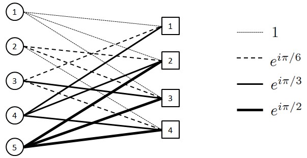
Figure 2: Property 1: Bipartite “approximate expander” graph with ${n}=5$ nodes on the left, and ${m}^{\prime}=4$ nodes on the right. Each node on the left has degree ${3}$. Property 2: The thicknesses of the edges represent the weights assigned to the edges. In particular, it is required that for each node on the right, the edges incoming have distinct weights. In this example, the thinnest edges are assigned a weight of $1$, the next thickest edges have a weight $e^{\iota\pi/6}$, the next thickest edges have weight $e^{\iota 2\pi/6}=e^{\iota\pi/3}$, and the thickest edges have weight $e^{\iota 3\pi/6}=e^{\iota\pi/2}$.

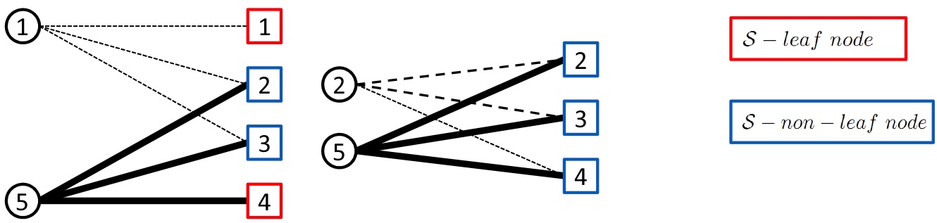
Figure 3: Property 3: We require that most sets ${\mathcal{S}}^{\prime}({\mathbf{x}})$ of at most $|{\mathcal{S}}({\mathbf{x}})|={k}=2$ nodes on the left in the graph $\mathcal{G}$ in Figure 2 have at least $2|{\mathcal{S}}^{\prime}({\mathbf{x}})|$ neighbors on the right. ) In the graph in Figure 2 it can be manually verified that most sets of size ${\mathcal{S}}^{\prime}({\mathbf{x}})$ at most $2$ have at least $2|{\mathcal{S}}^{\prime}({\mathbf{x}})|$ neighbors. For example, Figure 2(a) focuses on the subset ${\mathcal{S}}^{\prime}({\mathbf{x}})=\{1,5\}$ of nodes on the left side of $\mathcal{G}$ in Figure 2. This particular ${\mathcal{S}}^{\prime}({\mathbf{x}})$ has $4$ neighbours, and all its single-node subsets have $3$ neighbours. The only ${\mathcal{S}}^{\prime}({\mathbf{x}})$ set of two or fewer nodes that does not satisfy Property 3 is $\{2,5\}$, as shown in Figure 2(b), since it has only $3<2\times 2$ neighbours. Property 4: For sets ${\mathcal{S}}^{\prime}({\mathbf{x}})$ that satisfy Property 3 it can be manually verified that “many” of their neighbours are ${\mathcal{S}}^{\prime}({\mathbf{x}})$-leaf nodes. For example, for ${\mathcal{S}}^{\prime}({\mathbf{x}})=\{1,5\}$, two out of its four neighbours (i.e., a fraction $1/2$) are ${\mathcal{S}}^{\prime}({\mathbf{x}})$-leaf nodes – which satisfies the constraint that at least a fraction $1/2$ of its neighbours be ${\mathcal{S}}^{\prime}({\mathbf{x}})$-leaf nodes. On the other hand, for ${\mathcal{S}}^{\prime}({\mathbf{x}})=\{2,5\}$ (which does not satisfy Property 3), none of its neighbours are ${\mathcal{S}}^{\prime}({\mathbf{x}})$-leaf nodes.

$\Box$

We now state the Lemmas needed to make our arguments precise. First, we formalize the ${\mathcal{S}}^{\prime}({\mathbf{x}})$-expansion property defined in Property 3.

Lemma 1.

(Property 3 (${\mathcal{S}}({\mathbf{x}})$-expansion)): Let ${k}<{n}\in\bbn$ be arbitrary, and let ${c}\in\bbn$ be fixed. Let $\mathcal{G}$ be chosen uniformly at random from the set of all bipartite graphs with ${n}$ nodes (each of degree ${d}$) on the left and ${m}^{\prime}={c}{k}$ nodes on the right. Then for any ${\mathcal{S}}({\mathbf{x}})$ of size at most ${k}$ and any ${\mathcal{S}}^{\prime}({\mathbf{x}})\subseteq{\mathcal{S}}({\mathbf{x}})$, with probability $1-o(1/{k})$ (over the random choice $\mathcal{G}$) there are at least $2{d}/3$ times as many nodes neighbouring those in ${\mathcal{S}}^{\prime}({\mathbf{x}})$, as there are in ${\mathcal{S}}^{\prime}({\mathbf{x}})$.

Proof: Follows from a standard probabilistic method argument. Given for completeness in Appendix -A.

Note here that, in contrast to the “usual” definition of “vertex expansion” [48] (wherein the expansion property is desired “for all” subsets of left nodes up to a certain size) Lemma 1 above only gives a probabilistic expansion guarantee for any subset of ${\mathcal{S}}({\mathbf{x}})$ of size ${k}$. In fact, Lemma 2 below shows that for the parameters of interest, “for all”-type expanders cannot exist.

Lemma 2.

Let ${k}=o({n})$, and $d>0$ be an arbitrary constant. Let $\mathcal{G}$ be an arbitrary bipartite graph with ${n}$ nodes (each of degree $d$) on the left and ${m}^{\prime}$ nodes on the right. Then for all sufficiently large ${n}$, suppose each set of of size ${k}$ of ${\mathcal{S}}({\mathbf{x}})$ nodes on the left of $\mathcal{G}$ has strictly more than $d/2$ times as many nodes neighbouring those in ${\mathcal{S}}({\mathbf{x}})$, as there are in ${\mathcal{S}}({\mathbf{x}})$. Then ${m}^{\prime}=\Omega({k}\log({n}/{k}))$.

Proof: Follows from the Hamming bound in coding theory [47] and standard techniques for expander codes [36]. Proof in Appendix -B.

Another way of thinking about Lemma 2 is that it indicates that if one wants a “for all” guarantee on expansion, then one has to return to the regime of ${m}^{\prime}={\mathcal{O}}({k}\log({n}/{k}))$ measurements, as in “usual” compressive sensing.

Next, we formalize the “many ${\mathcal{S}}({\mathbf{x}})$-leaf nodes” property defined in Property 4. Recall that for any set ${\mathcal{S}}({\mathbf{x}})$ of at most ${k}$ nodes on the left of $\mathcal{G}$, we call any node on the right of $\mathcal{G}$ an ${\mathcal{S}}({\mathbf{x}})$-leaf node if it has exactly one neighbor in ${\mathcal{S}}({\mathbf{x}})$.

Lemma 3.

Let ${\mathcal{S}}({\mathbf{x}})$ be a set of ${k}$ nodes on the left of $\mathcal{G}$ such that the number of nodes neighbouring those in any ${\mathcal{S}}^{\prime}({\mathbf{x}})\subseteq{\mathcal{S}}({\mathbf{x}})$ is at least $2{d}/3$ times the size of ${\mathcal{S}}^{\prime}({\mathbf{x}})$. Then at least a fraction $1/2$ of the nodes that are neighbours of any ${\mathcal{S}}^{\prime}({\mathbf{x}})\subseteq{\mathcal{S}}({\mathbf{x}})$ are ${\mathcal{S}}^{\prime}({\mathbf{x}})$-leaf nodes.

Proof: Based on Lemma 1. Follows from a counting argument similar to those used in expander codes [36]. Proof in Appendix -C.

Given a graph $\mathcal{G}$ satisfying properties 1-4, we now describe our encoding and decoding procedure.

II-C Measurement design

Matrix structure and entries: The encoder’s measurement matrix ${{A}}$ is chosen based on the structure of $\mathcal{G}$ (recall that $\mathcal{G}$ has ${n}$ nodes on the left and ${m}^{\prime}$ nodes on the right). To begin with, the matrix ${{A}}$ has ${m}=2{m}^{\prime}$ rows, and its non-zero values are unit-norm complex numbers.

Remark 1.

This choice of using complex numbers rather than real numbers in ${{A}}$ is for notational convenience only. One equally well choose a matrix ${{A}}^{\prime}$ with ${m}=4{m}^{\prime}$ rows, and replace each row of ${{A}}$ with two consecutive rows in ${{A}}^{\prime}$ comprising respectively of the real and imaginary parts of rows of ${{A}}$. Since the components of ${\mathbf{x}}$ are real numbers, hence there is a bijection between ${{A}}{\mathbf{x}}$ and ${{A}}^{\prime}{\mathbf{x}}$ – indeed, consecutive pairs of elements in ${{A}}^{\prime}{\mathbf{x}}$ are respectively the real and imaginary parts of the complex components of ${{A}}{\mathbf{x}}$. Also, as we shall see (in Section II-H5), the choice of unit-norm complex numbers ensures that “noise” due to finite precision arithmetic does not get “amplified”. In Section II-H6, we argue that this property enables us to apply SHO-FA to other settings such as wireless systems that naturally generate an ensemble of matrices that resemble SHO-FA.

In particular, corresponding to node ${i}$ on the right-hand side of $\mathcal{G}$, the matrix ${{A}}$ has two rows. The ${j}^{th}$ entries of the $(2{i}-1)^{th}$ and $2{i}^{th}$ rows of ${{A}}$ are respectively denoted $a_{{i},{j}}^{(I)}$ and $a_{{i},{j}}^{(V)}$ respectively. (The superscripts $(I)$ and $(V)$ respectively stand for Identification and Verification, for reasons that shall become clearer when we discuss the process to reconstruct ${\mathbf{x}}$.)

Identification entries: If $\mathcal{G}$ has no edge connecting node ${j}$ on the left with ${i}$ on the right, then the identification entry $a_{{i},{j}}^{(I)}$ is set to equal $0$. Else, if there is indeed such an edge, $a_{{i},{j}}^{(I)}$ is set to equal

$$a_{{i},{j}}^{(I)}=e^{\iota{j}\pi/(2{n})}.$$ (1)

(Here $\iota$ denotes the positive square root of $-1$.) This entry $a_{{i},{j}}^{(I)}$ can also be thought of as the weight of the edge in $\mathcal{G}$ connecting ${j}$ on the left with ${i}$ on the right. In particular, the phase ${j}\pi/(2{n})$ of $a_{{i},{j}}^{(I)}=e^{\iota{j}\pi/(2{n})}$ will be critical for our algorithm. As in Property 2 in Section II-B, our choice above guarantees distinct weights for all edges connected to a node ${i}$ on the right.

Verification entries: Whenever the identification entry $a_{{i},{j}}^{(I)}$ equals $0$, we choose to set the corresponding verification entry $a_{{i},{j}}^{(V)}$ also to be zero. On the other hand, whenever $a_{{i},{j}}^{(I)}\neq 0$, then we set $a_{{i},{j}}^{(V)}$ to equal $e^{\iota\theta_{{i},{j}}^{(V)}}$ for $\theta_{{i},{j}}^{(V)}$ chosen uniformly at random from $[0,\pi/2]$ (with ${\mathcal{O}}(\log({k}))$ bits of precision).

Example $2$: The matrix ${{A}}$ corresponding to the graph $\mathcal{G}$ in Example $1$ is show in Figure 4.

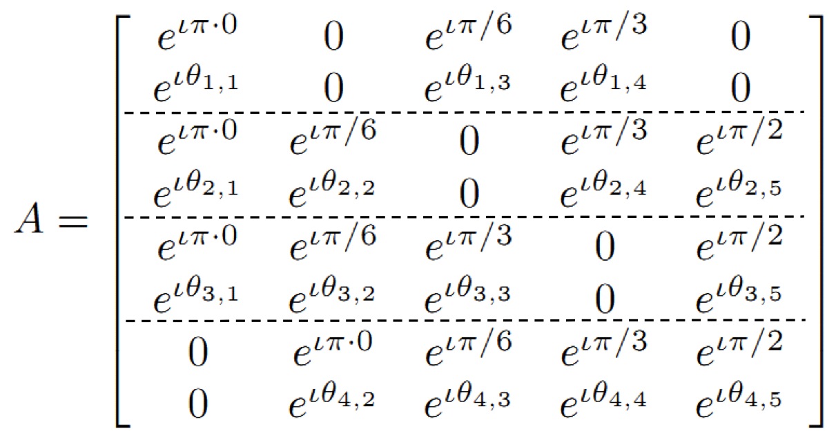
Figure 4: This $8\times 5$ matrix denotes the ${{A}}$ corresponding to the graph $\mathcal{G}$. Note that its primary purpose is expository – clearly, $8$ measurements (or indeed, $16$ measurements over ) to reconstruct a $2$-sparse vector of length $5$ is too many! Nonetheless, this is just an artifact of the fact that ${n}$ in this example is small. In fact, according to our proofs, even as ${n}$ scales to infinity, the number of measurements required to reconstruct a $2$-sparse vector (or in general a ${k}$-sparse vector for constant ${k}$) remains constant! Also, note that we do not use the assignment for the identification entries $a_{{i},{j}}^{(I)}$ specified in (1), since doing so would result in ugly and not very illuminating calculations in Example $3$ below. However, as noted in Remark 2, this is not critical – it is sufficient that distinct entries in the identification rows of the matrix be distinct.

II-D Reconstruction

II-D1 Overview

We now provide some high-level intuition on the decoding process.

Since the measurement matrix ${{A}}$ has interspersed identification and verification rows, this induces corresponding interspersed identification observations $y_{{i}}^{(I)}$ and verification verifications observations $y_{{i}}^{(V)}$ in the observation vector ${\mathbf{y}}={{A}}{\mathbf{x}}$. Let ${\mathbf{y}}^{(I)}=\{y_{{i}}^{(I)}\}$ denote the length-${m}$ identification vector over , and ${\mathbf{y}}^{(V)}=\{y_{{i}}^{(V)}\}$ denote the length-${m}$ verification vector over .

Given the measurement matrix ${{A}}$ and the observed $({\mathbf{y}}^{(I)},{\mathbf{y}}^{(V)})$ identification and verification vectors, the decoder’s task is to find any “consistent” ${k}$-sparse vector $\hat{{\mathbf{x}}}$ such that ${{A}}\hat{{\mathbf{x}}}$ results in the corresponding identification and verification vectors. We shall argue below that if we succeed, then with high probability over ${{A}}$ (specifically, over the verification entries of ${{A}}$), this $\hat{{\mathbf{x}}}$ must equal ${\mathbf{x}}$.

To find such a consistent $\hat{{\mathbf{x}}},$ we design an iterative decoding scheme. This scheme starts by setting the initial guess for the reconstruction vector $\hat{{\mathbf{x}}}$ to the all-zero vector. It then initializes, in the manner described in the next paragraph, a ${\mathcal{S}}({\mathbf{x}})$-leaf-node list, $\mathcal{L}(1)$, a set of indices of ${\mathcal{S}}({\mathbf{x}})$-leaf nodes.

The decoder checks to see whether ${i}$ is a ${\mathcal{S}}({\mathbf{x}})$-leaf node in the following way. First, it looks at the entry $y_{{i}}^{(I)}$ and “estimates” which node ${j}$ on the left of the graph $\mathcal{G}$ “could have generated the identification observation $y_{{i}}^{(I)}$”. It then uses the verification entry $a_{{i},{j}}^{(V)}$ and the verification observation $y_{{i}}^{(V)}$ to verify its estimate. After sequentially examining each entry $y_{{i}}^{(I)}$, the list of all ${\mathcal{S}}({\mathbf{x}})$-leaf nodes is denoted $\mathcal{L}(1)$.

In the ${t}^{th}$ iteration of the decoding process, the decoder picks a leaf node in ${i}\in\mathcal{L}(t)$. Using this, it then reconstructs the non-zero component $x_{{j}}$ of ${\mathbf{x}}$ that “generated” $y_{{i}}^{(I)}$. If this reconstructed value $x_{{j}}$ is successfully “verified” using the verification entry $a_{{i},{j}}^{(V)}$ and the verification observation $y_{{i}}^{(V)}$), then the algorithm performs the following steps in this iteration:

• It updates the observation vectors by subtracting the “contribution” of the coordinate $x_{{j}}$ to the measurements it influences (there are exactly $7$ of them since the degree of the nodes on the left side of $\mathcal{G}$ is $7$).

• It updates the ${\mathcal{S}}({\mathbf{x}})$-leaf-node list, $\mathcal{L}(t)$ by removing ${i}$ from $\mathcal{L}(t)$ and checking the change of status (zero, leaf, or non-leaf) of other indices influenced by $x_{{j}}$ (there at most $6$),

• Finally the algorithm picks a new index ${i}$ from the updated list, $\mathcal{L}(t+1)$ for the next iteration.

The decoder performs the above operations repeatedly until $\hat{{\mathbf{x}}}$ has been completely recovered. We also show that (with high probability over ${{A}}$) in at most ${k}$ steps this process does indeed terminate.

Example $3$: Figures 5–9 show a sample decoding process for the matrix ${{A}}$ as in Example $2$, and the observed vector ${\mathbf{y}}$ shown in the figures. The example also demonstrates each of several possible scenarios the algorithm can find itself in, and how it deals with them.

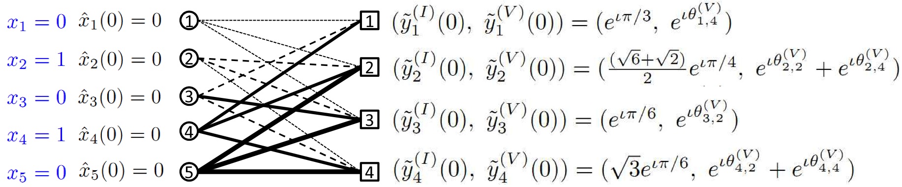
Figure 5: Initialization: The (true) ${\mathbf{x}}$ equals $(0,1,0,1,0)$ (and hence ${\mathcal{S}}({\mathbf{x}})=\{2,4\}$). Also note that nodes $1$ and $3$ on the right of $\mathcal{G}$ are ${\mathcal{S}}({\mathbf{x}})$-leaf nodes, as defined in Property 4. However, all of this is unknown to the decoder a priori. The decoder sets the (starting) estimate $\hat{{\mathbf{x}}}(0)$ of the reconstruction vector $\hat{{\mathbf{x}}}$ to the all-zeros vector. The (starting) gap vector $\tilde{{\mathbf{y}}}$ is set to equal ${\mathbf{y}}$, which in turn equals the corresponding $4$ pairs of identification and verification observations on the right-hand side of $\mathcal{G}$. The specific values of $\theta_{i,j}^{(V)}$ in the verification observations do not matter currently – all that matters is that given ${\mathbf{x}}$, each of the four verification observations are non-zero (with high probability over the choices of $\theta_{i,j}^{(V)}$). Hence the (starting) value of the neighbourly set equals $\{1,2,3,4\}$. This step takes ${\mathcal{O}}({k})$ number of steps, just to initialize the neighbourly set. By the end of the decoding algorithm (if it runs successfully), the tables will be turned – all the entries on the right of $\mathcal{G}$ will equal zero, and (at most) ${k}$ entries on the left of $\mathcal{G}$ will be non-zero.

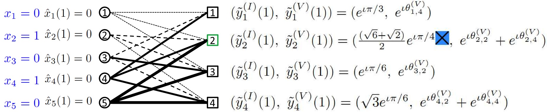
Figure 6: Leaf-Node List 1 (Failed identification): The decoder picks the index ${i}=2$ from the neighbourly set $\{1,2,3,4\}$, and checks the phase of the corresponding gap vector identification observation $\tilde{y}_{2}^{(I)}$. Since this equals $\pi/4$, which is not in the set of possible phases in the $2^{nd}$ identification row of ${{A}}$ (which are all multiples of $\pi/6$), the decoder declares ${i}=2$ is not a leaf node. This entire process takes a constant number of steps.

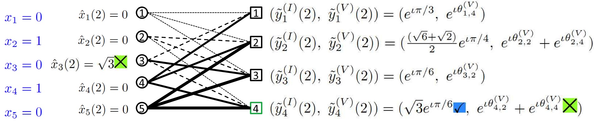
Figure 7: Leaf-Node List 2 (Passed identification, failed verification): In this step, a potentially more serious failure could happen. In particular, suppose the decoder picks the index ${i}=4$ from the neighbourly set $\{1,2,3,4\}$ (note that $4$ is also not a ${\mathcal{S}}({\mathbf{x}})$-leaf node), and checks the phase of the corresponding gap vector identification observation $\tilde{y}_{4}^{(I)}$, it just so happens that the value of ${\mathbf{x}}$ is such that this corresponds to a phase of $\pi/6$. But as can be seen from the matrix in Figure 4, for ${i}=4$ this corresponds to $a_{{i},{j}}^{(I)}$ for ${j}=3$. Hence the decoder would make a “false identification” of ${j}=3$, and estimate that $\hat{x}_{3}$ equals the magnitude of $\tilde{y}_{4}^{(I)}$, which would equal $\sqrt{3}$. This is where the verification entries and verification observations save the day. Recall that the phase of each verification entry is chosen uniformly at random (with sufficient bit precision) from $[0,\pi/2)$, independently of both ${\mathbf{x}}$ and the other entries of ${{A}}$. Hence the probability that $\sqrt{3}$ (the misdirected value of $\hat{x}_{3}$) times the corresponding verification entry $a_{4,3}^{(V)}$ equals $\tilde{y}_{4}^{(I)}$ is “small”. Hence the decoder in this case too declares ${i}=4$ is not a leaf node. This entire process takes a constant number of steps.

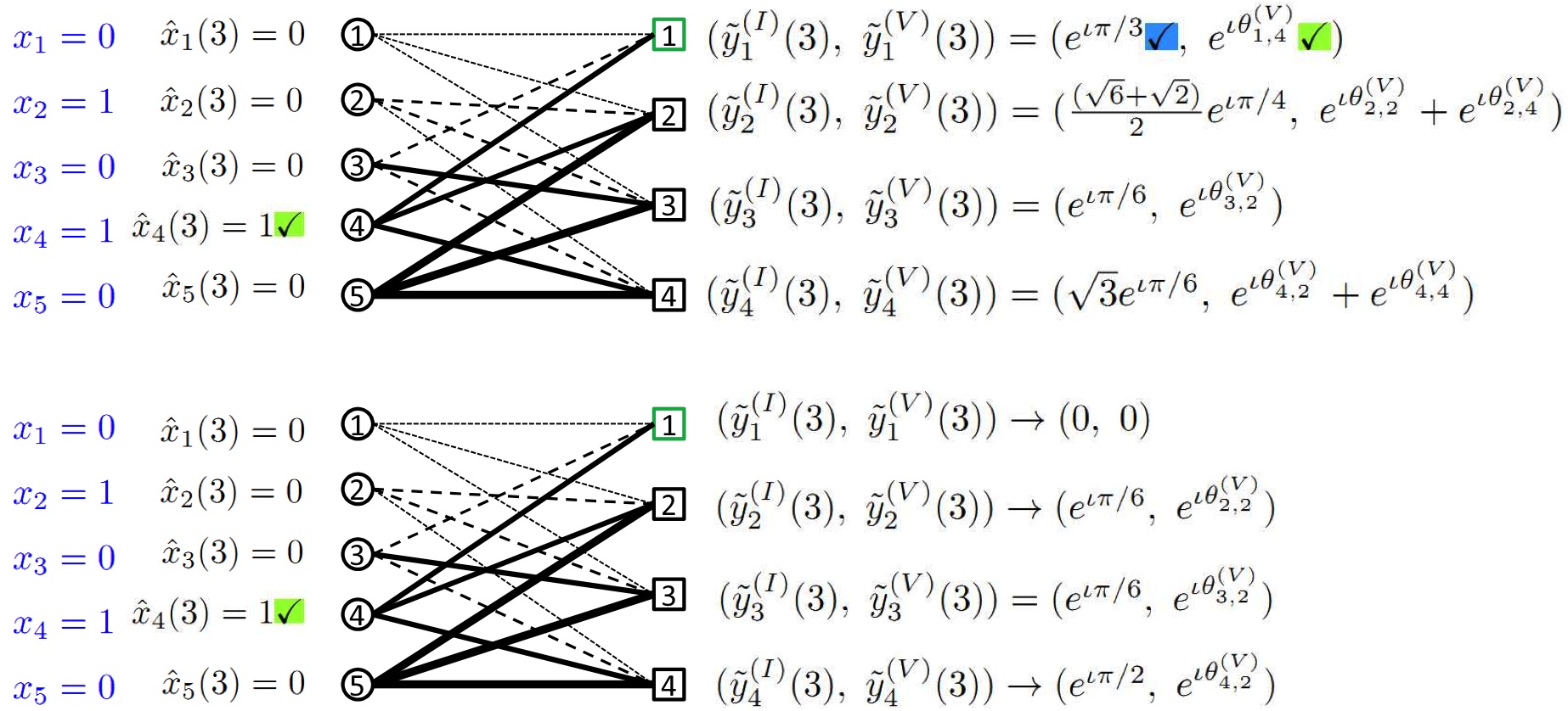
Figure 8: Leaf-Node List 3 (Passed identification, passed verification) and the first iteration: Now, suppose the decoder randomly picks the index ${i}=1$ from the neighbourly set $\{1,2,3,4\}$ (note that $1$ is a ${\mathcal{S}}({\mathbf{x}})$-leaf node). In this case, the phase of the corresponding gap vector identification observation $\tilde{y}_{1}^{(I)}$ equals $\pi/3$. As can be seen from the matrix in Figure 4, for ${i}=1$ this corresponds to $a_{{i},{j}}^{(I)}$ for ${j}=4$. Hence the decoder makes a “correct identification” of ${j}=4$, and estimates (also correctly) that $\hat{x}_{4}$ equals the magnitude of $\tilde{y}_{1}^{(I)}$, which equals $1$. On checking with the verification entry, the decoder observes also that $1$ (the detected value of $\hat{x}_{4}$) times the corresponding verification entry $a_{1,4}^{(V)}$ equals $\tilde{y}_{1}^{(V)}$. Hence it declares that ${i}=1$ is a leaf node. Similarly, we know that $3$ is a leaf node too. Therefore, the leaf node set equals $\{1,3\}$. The entire process of making a list of leaf node takes ${\mathcal{O}}({k})$ number of steps. Suppose in the first iteration, the decoder picks ${i}=1$. Hence it updates the value of $\hat{x}_{4}$ to $1$, the neighbourly set to $\{2,3,4\}$, the leaf node set to $\{2,3,4\}$ and $\tilde{{\mathbf{y}}}$ to the values shown (only the three indices $1$, $3$ and $4$ on the right need to be changed). At this point, note that ${\mathcal{S}}^{\prime}({\mathbf{x}})$ also changes from $\{2,4\}$ to the singleton set $\{4\}$. This entire iteration takes a constant number of steps.

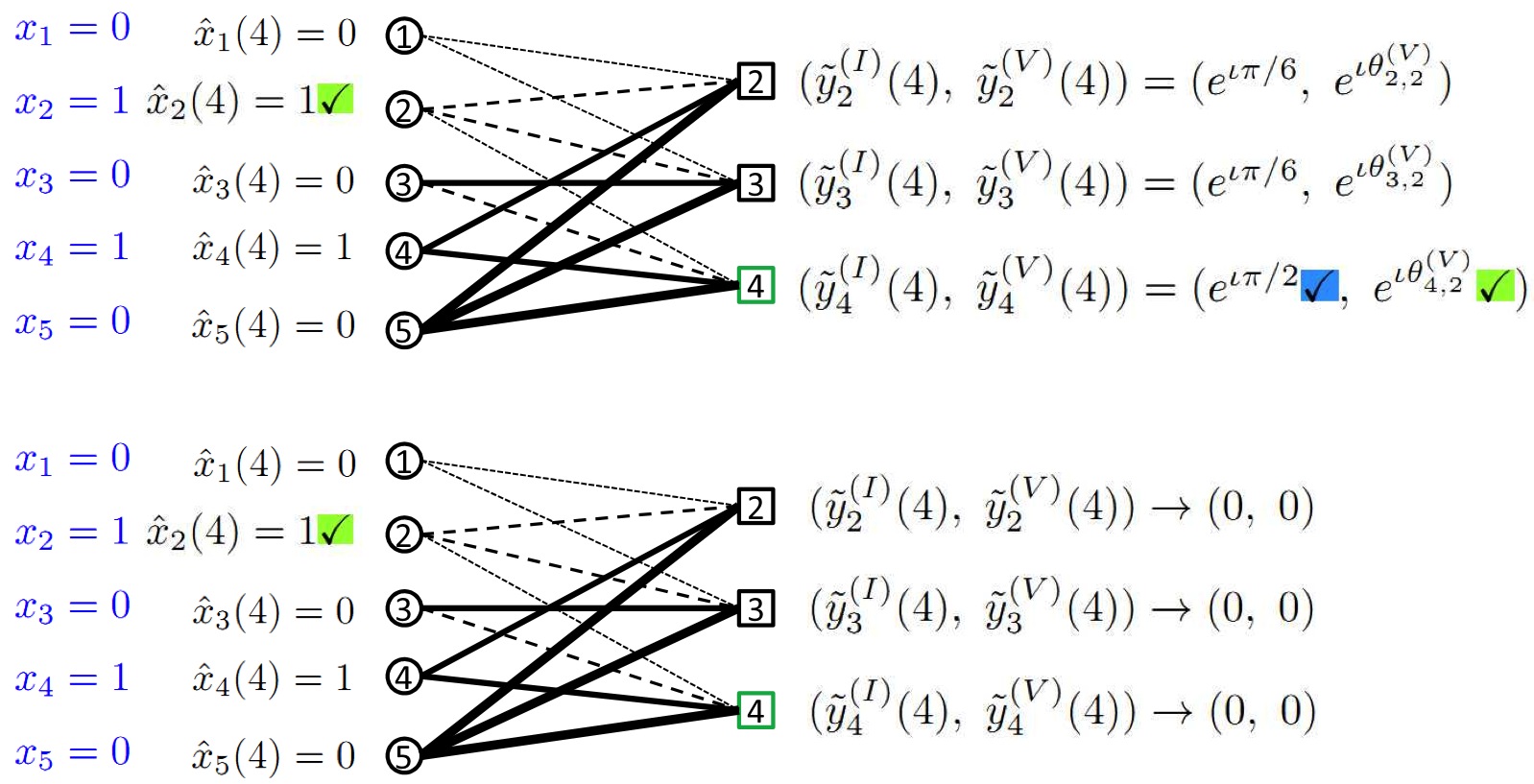
Figure 9: Second iteration and Termination: In the second iteration, the decoder randomly picks ${i}=4$ from the leaf node set $\{2,3,4\}$. Recall that in the first iteration this choice of ${i}$ did not aid in decoding. However, now that node $4$ on the right of $\mathcal{G}$ has been “cleaned up”, it is now a leaf node for ${\mathcal{S}}^{\prime}({\mathbf{x}})$. This demonstrates the importance of not “throwing away” information which seems useless at some point in time. Hence, analogously to the process in Figure 8, the decoder estimates the value of $\hat{x}_{2}$ to $1$, updates the leaf node set to the empty set, and $\tilde{{\mathbf{y}}}$ to the all-zero vector (all in a constant number of steps). Since the gap vector is zero, this indicates to the decoder that it should output $\hat{{\mathbf{x}}}$ as its estimate of ${\mathbf{x}}$, and terminate.

II-D2 Formal description of SHO-FA’s reconstruction process

Our algorithm proceeds iteratively, and has at most ${k}$ overall number of iterations, with ${t}$ being the variable indexing the iteration number.

1. Initialization: We initialize by setting the signal estimate vector $\hat{{\mathbf{x}}}{(1)}$ to the all-zeros vector $0^{{n}}$, and the residual measurement identification/verification vectors $\tilde{{\mathbf{y}}}^{(I)}(1)$ and $\tilde{{\mathbf{y}}}^{(V)}(1)$ to the decoder’s observations ${\mathbf{y}}^{(I)}$ and ${\mathbf{y}}^{(V)}$.

2. Leaf-Node List: Let $\mathcal{L}(1)$, the initial ${\mathcal{S}}({\mathbf{x}})$-leaf node set, be the set of indices ${i}$ which are ${\mathcal{S}}({\mathbf{x}})$-leaf nodes. We generate the list via the following steps:

   1. Compute angles $\theta^{(I)}({i})$ and $\theta^{(V)}({i})$: Let the identification and verification angles be defined respectively as the phases of the identification and verification entries being considered for index $i$ (starting from 1), as follows:

      $$\theta^{(I)}({i}) \triangleq \angle\left(\tilde{y}_{i}^{(I)}(1)\right),$$

      $$\theta^{(V)}({i}) \triangleq \angle\left(\tilde{y}_{i}^{(V)}(1)\right).$$

      Here $\angle(.)$ computes the phase of a complex number (up to ${\mathcal{O}}(\max\{\log{{n}/{k}},\log({k}))\})$ bits of precision).

   2. Check if the current identification and verification angles correspond to a valid and unique $x_{{j}}$: For this, we check at most two things (both calculations are done up to the precision specified in the previous step).

      1. First, we check if ${j}\triangleq\theta^{(I)}(i)(2{n}/\pi)$ is an integer, and the corresponding ${j}^{th}$ element of the ${i}^{th}$ row is non-zero. If so, we have “tentatively identified” that the ${i}^{th}$ component of $\tilde{{\mathbf{y}}}$ is a leaf-node of the currently unidentified non-zero components of ${\mathbf{x}}$, and in particular is connected to the ${j}^{th}$ node on the left, and the algorithm proceeds to the next step below. If not, we simply increment ${i}$ by $1$ and return to Step (2a).

      2. Next, we verify our estimate from the previous step. If $a_{{i},{j}}^{(V)}\tilde{y}_{i}^{(I)}/a_{{i},{j}}^{(I)}=\tilde{y}_{i}^{(V)}$, the verification test passes, and include ${i}$ in $\mathcal{L}(1)$. If not, we simply increment ${i}$ by $1$ and return to Step (2a).

3. Operations in ${t}^{th}$ iteration: The ${t}^{th}$ decoding iteration accepts as its input the ${t}^{th}$ signal estimate vector $\hat{{\mathbf{x}}}{({t})}$, the ${t}^{th}$ leaf node set $\mathcal{L}({t})$, and the ${t}^{th}$ residual measurement identification/verification vectors $(\tilde{{\mathbf{y}}}^{(I)}{({t})},\tilde{{\mathbf{y}}}^{(V)}{({t})})$. In ${\mathcal{O}}(1)$ steps it outputs the $({t}+1)^{th}$ signal estimate vector $\hat{{\mathbf{x}}}{({t}+1)}$, the $({t}+1)^{th}$ leaf node set $\mathcal{L}({t}+1)$, and the $({t}+1)^{th}$ residual measurement identification/verification vectors $(\tilde{{\mathbf{y}}}^{(I)}{({t}+1)},\tilde{{\mathbf{y}}}^{(V)}{({t}+1)})$ after the performing the following steps sequentially (each of which takes at most a constant number of atomic steps):

   1. Pick a random ${i}{({t})}\in\mathcal{L}({t})$: The decoder picks an element ${i}{({t})}$ uniformly at random from the ${t}^{th}$ leaf-node list $\mathcal{L}({t})$.

   2. Compute angles $\theta^{(I)}({{t}})$ and $\theta^{(V)}({{t}})$: Let the current identification and verification angles be defined respectively as the phases of the residual identification and verification entries being considered in that step, as follows:

      $$\theta^{(I)}({t}) \triangleq \angle\left(\tilde{y}_{i{({t})}}^{(I)}{({t})}\right),$$

      $$\theta^{(V)}({t}) \triangleq \angle\left(\tilde{y}_{i{({t})}}^{(V)}{({t})}\right).$$

   3. Locate non-zero entry ${j}$ and derive the value of $\hat{x}_{{j}{({t})}}{({t})}$: For this, we do at most two things (both calculations are done up to the precision specified in the previous step).

      1. First, we calculate ${j}{({t})}\triangleq\theta^{(I)}({t})(2{n}/\pi)$. We have identified that the ${i}^{th}$ component of $\tilde{{\mathbf{y}}}$ is a leaf-node of the currently unidentified non-zero components of ${\mathbf{x}}$, and in particular is connected to the ${j}{({t})}^{th}$ node on the left, and the algorithm proceeds to the next step below.

      2. Next, we assign the value, $\tilde{y}_{i{({t})}}^{(I)}{({t})}/a_{{i}{({t})},{j}{({t})}}^{(I)}=\tilde{y}_{i{({t})}}^{(V)}{({t})}/a_{{i}{({t})},{j}{({t})}}^{(V)}$, to $\hat{x}_{{j}{({t})}}{({t})}$ and proceeds the algorithm to the next step below.

   4. Update $\hat{{\mathbf{x}}}{({t}+1)}$, $\mathcal{L}(t+1)$ ,$\tilde{{\mathbf{y}}}^{(I)}{({t}+1)}$, and $\tilde{{\mathbf{y}}}^{(V)}{({t}+1)}$: In particular, at most $7$ components of each of these vectors need to be updated. Specifically, $\hat{x}_{{j}{({t})}}{({t}+1)}$ equals $\tilde{y}_{i{({t})}}^{(I)}{({t})}/a_{{i}{({t})},{j}{({t})}}^{(I)}$. ${i}{({t})}$ is removed from the leaf node set $\mathcal{L}(t)$ and check whether the (at most six) neighbours of $\hat{x}_{{j}{({t})}}{({t})}$ become leaf node to get the leaf-node list $\mathcal{L}(t+1)$. And finally (seven) values each of $\tilde{{\mathbf{y}}}^{(I)}{({t}+1)}$ and $\tilde{{\mathbf{y}}}^{(V)}{({t}+1)}$ are updated from those of $\tilde{{\mathbf{y}}}^{(I)}{({t})}$ and $\tilde{{\mathbf{y}}}^{(V)}{({t})}$ (those corresponding to the neighbours of $\hat{x}_{{j}{({t})}}{({t})}$) by subtracting out $\hat{x}_{{j}{({t})}}{({t})}$ multiplied by the appropriate coefficients of ${{A}}$.

4. Termination: The algorithm stops when the leaf node set is empty, and outputs the last $\hat{{\mathbf{x}}}({t})$.

II-E Decoding complexity

We start by generating $\mathcal{L}(1)$, the initial list of leaf nodes. For each node $i$, we calculate the identification and verification angles (which takes $2$ operations), and then check if the identification and verification angles correspond to a valid and unique $x_{j}$ (which takes $2$ operations). Therefore generating the initial list of leaf nodes takes ${\mathcal{O}}({k})$ (to be precise $4c{k}$) operations .

In iteration ${t}$, we decode a new non-zero entry $x_{j}$ of ${\mathbf{x}}$ by picking a leaf node from $\mathcal{L}({t})$, identifying the corresponding index ${j}$ and value $x_{j}$ (via $2$ arithmetic operations corresponding to the identification and verification steps respectively), and updating $\mathcal{L}({t}+1)$ (since $x_{j}$ is connected to $3$ nodes on the right, out of which one has already been decoded, this takes at most $4$ operations – $2$ for identification and $2$ for verification), $\tilde{{\mathbf{y}}}^{(I)}{({t}+1)}$, and $\tilde{{\mathbf{y}}}^{(V)}{({t}+1)}$ (similarly, this takes at most $8$ operations – $4$ additions and $4$ multiplications).

Next we note that each iteration results in recovering a new non-zero coordinate of ${\mathbf{x}}$ (assuming no decoding errors, which it true with high probability as demonstrated in the next section). Hence the total number of iterations is at most ${k}$.

Hence the overall number of operations over all iterations is ${\mathcal{O}}({k})$ (to be precise, at most $4c{k}+14{k}$).

II-F Correctness

Next, we show that $\hat{{\mathbf{x}}}={\mathbf{x}}$ with high probability over ${{A}}$. To show this, it suffices to show that each non-zero update to the estimate $\hat{{\mathbf{x}}}{({t})}$ sets a previously zero coordinate to the correct value with sufficiently high probability.

Note that if ${i}{({t})}$ is a leaf node for ${\mathcal{S}}{({t})}$, and if all non-zero coordinates of $\hat{{\mathbf{x}}}{({t})}$ are equal to the corresponding coordinates in ${\mathbf{x}}$, then the decoder correctly identifies the parent node $j{({t})}\in{\mathcal{S}}{({t})}$ for the leaf node ${i}{({t})}$ as the unique coordinate that passes the phase identification and verification checks.

Thus, the ${t}^{th}$ iteration ends with an erroneous update only if

$$\angle\left(\sum_{p\in N(\{{i}{({t})}\})}x_{p}e^{\iota\theta_{i(t),p}^{(I)}}\right)=\theta_{i(t),j(t)}^{(I)}$$

for some ${j}$ such that there are more than one non-zero terms in the summation on the left.

$$\angle\left(\sum_{p\in N(\{{i}{({t})}\})}x_{p}e^{\iota\theta_{i(t),p}^{(V)}}\right)=\theta_{i(t),j(t)}^{(V)}$$

Since $\theta_{i(t),j(t)}^{(V)}$ is drawn uniformly at random from $[1,2,\ldots,\pi/2]$ (with $\Omega(\log({n})+P)={\mathcal{O}}(\log({k}))$ (say) bits of precision), the probability that the second equality holds with more than one non-zero term in the summation on the left is at most $o(1/poly({k}))$. The above analysis gives an upper bound on the probability of incorrect update for a single iteration to be $o(1/poly({k}))$. Finally, as the total number of updates is at most ${k}$, by applying a union bound over the updates, the probability of incorrect decoding is bounded from above by $o(1/poly({k}))$.

II-G Remarks on the Reconstruction process for exactly ${k}$-sparse signals

We elaborate on these choices of entries of ${{A}}$ in the remarks below, which also give intuition about the reconstruction process outlined in Section II-D2.

Remark 2.

In fact, it is not critical that (1) be used to assign the identification entries. As long as ${j}$ can be “quickly” (computationally efficiently) identified from the phases of $a_{{i},{j}}^{(I)}$ (as outlined in Remark 3 below, and specified in more detail in Section II-D2), this suffices for our purpose. This is the primary reason we call these entries identification entries.

Remark 3.

The reason for the choice of phases specified in (1) is as follows. Suppose ${\mathcal{S}}({\mathbf{x}})$ corresponds to the support (set of non-zero values) of ${\mathbf{x}}$. Suppose $y_{{i}}$ corresponds to a ${\mathcal{S}}({\mathbf{x}})$-leaf node, then by definition $y_{{i}}^{(I)}$ equals $a_{{i},{j}}^{(I)}x_{{j}}$ for some ${j}$ in $\{1,\ldots,{n}\}$ (if $y_{{i}}$ corresponds to a ${\mathcal{S}}({\mathbf{x}})$-non-leaf node, then in general $y_{{i}}^{(I)}$ depends on two or more $x_{{j}}$). But $x_{{j}}$ is a real number. Hence examining the phase of $y_{{i}}$ enables one to efficiently compute ${j}\pi/(2{n})$, and hence ${j}$. It also allows one to recover the magnitude of $x_{{j}}$, simply by computing the magnitude of $y_{{i}}$.

Remark 4.

The choice of phases specified in (1) divides the set of allowed phases (the interval $[0,\pi/2]$) into ${n}$ distinct values. Two things are worth noting about this choice.

1. We consider the interval $[0,\pi/2]$ rather than the full range $[0,2\pi)$ of possible phases since we wish to use the phase measurements to also recover the sign of $x_{{j}}$s. If the phase of $y_{{i}}$ falls within the interval $[0,\pi/2]$, then (still assuming that $y_{{i}}$ corresponds to a ${\mathcal{S}}({\mathbf{x}})$-leaf node) $x_{{j}}$ must have been positive. On the other hand, if the phase of $y_{{i}}$ falls within the interval $[\pi,3\pi/2]$, then $x_{{j}}$ must have been negative. (It can be directly verified that the phase of a ${\mathcal{S}}({\mathbf{x}})$-leaf node $y_{{i}}$ can never be outside these two intervals – this wastes roughly half of the set of possible phases we could have used for identification purposes, but it makes notation easier.

2. The choice in (1) divides the interval $[0,\pi/2]$ into ${n}$ distinct values. However, in expectation over $\mathcal{G}$ the actual number of non-zero entries in a row of ${{A}}$ is ${\mathcal{O}}({n}/{k})$, so on average one only needs to choose ${\mathcal{O}}({n}/{k})$ distinct phases in (1), rather than the worst case ${n}$ number of values. This has the advantage that one only needs ${\mathcal{O}}(\log({n}/{k}))$ bits of precision to specify distinct phase values (and in fact we claim that this is the level of precision required by our algorithm). However, since we analyze only left-regular $\mathcal{G}$, the degrees of nodes on the right will in general vary stochastically around this expected value. If ${k}$ is “somewhat large” (for instance ${k}=\Omega({n})$), then the degrees will not be very tightly concentrated around their mean. One way around this is to choose $\mathcal{G}$ uniformly at random from the set of bipartite graphs with ${n}$ nodes (each of degree ${d}$) on the left and ${m}$ nodes (each of degree ${d}{n}/{m}$) on the right. This would require a more intricate proof of the ${\mathcal{S}}^{\prime}({\mathbf{x}})$-expansion property defined in Property 3 and proved in Lemma 1. For the sake of brevity, we omit this proof here.

Remark 5.

In fact, the recent work of [35] demonstrates an alternative analytical technique (bypassing the expansion arguments outlined in this work), involving analysis of properties of the “$2$-core” of random hyper-graphs, that allows for a tight characterization of the number of measurements required by SHO-FA to reconstruct ${\mathbf{x}}$ from ${\mathbf{y}}$ and ${{A}}$, rather than the somewhat loose (though order-optimal) bounds presented in this work. Since our focus in this work is a simple proof of order-optimality (rather than the somewhat more intricate analysis required for the tight characterization) we again omit this proof here.

II-H Other properties of SHO-FA

II-H1 SHO-FA v.s. “$2$-core” of random hyper-graphs

We reprise some concepts pertaining to the analysis of random hypergraphs (from [50]), which are relevant to our work.
$2$-cores of $d$-uniform hypergraphs: A $d$-uniform hypergraph with $m$ nodes and $k$ hyperedges is defined over a set of $m$ nodes, with each $d$-uniform hyperedge corresponding to a subset of the nodes of size exactly $d$. The $2$-core is defined as the largest sub-hypergraph (subset of nodes, and hyperedges defined only on this subset) such that each node in this subset is contained in at least $2$ hyperedges on this subset.

A standard “peeling process” that computationally efficiently finds the $2$-core is as follows: while there exists a node with degree $1$ (connected to just one hyperedge), delete it and the hyperedges containing it.

The relationship between $2$-cores in $d$-uniform hypergraphs and SHO-FA: As in [35] and other works, there exists bijection between $d$-uniform hypergraphs and $d$-left-regular bipartite graphs, which can be constructed as follows:

1. Each hyperedge in the hypergraph is mapped to a left node in the bipartite graph,

2. Each node in the hypergraph is mapped to a right node in the bipartite graph,

3. The edges leaving a left-node in the bipartite graph correspond to the nodes contained in the corresponding hyperedge of the hypergraph.

Suppose the $d$-uniform hypergraph does not contain a $2$-core. This means that, in each iteration of “peeling process”, we can find a vertex with degree $1$, delete it and the corresponding hyperedges. and continue the iterations until all the hyperedges are deleted. Correspondingly, in the bipartite graph, we can find a leaf node in each iteration, delete it and the corresponding left node and continue the iterations until all left nodes are deleted. We note that the SHO-FA algorithm follows essentially the same process. This implies that SHO-FA succeeds if and only if the $d$-uniform hypergraph contains a $2$-core.

Existence of 2-cores in d-uniform hypergraphs and SHO-FA: We now reprise a nice result due to [50] that helps us tighten the results of Theorem 1.

Theorem 2.

([50]) Let $d+l>4$ and $G$ be a $d$-uniform random hypergraph with $k$ hyperedges and $m$ nodes. Then there exists a number $c_{d,l}^{*}$ (independent of $k$ and $m$ that is the threshold for the appearance of an $l$-core in $G$. That is, for constant $c$ and $m\rightarrow\infty$: If $k/m=c<c_{d,l}^{*}$, then $G$ has an empty $l$-core with probability $1-o(1)$;If $k/m=c>c_{d,l}^{*}$, then $G$ has an $l$-core of linear size with probability $1-o(1)$.

Specifically, the results in [35, Theorem 1] (which explicitly calculates some of the $c_{d,l}^{*}$) give that for $l=2$ and $d=3$, $c_{3,2}^{*}=1/1.22$ with probability $1-{\mathcal{O}}(1/{k})$. This leads to the following theorem, that has tighter parameters than Theorem 1.

Theorem 3.

Let ${k}\leq{n}$. There exists a reconstruction algorithm SHO-FA for ${{A}}\in{}^{{m}\times{n}}$ with the following properties:

1. For every ${\mathbf{x}}\in\mathbb{R}^{{n}}$, with probability $1-{\mathcal{O}}(1/{k})$ over the choice of ${{A}}$, SHO-FA produces a reconstruction $\hat{{\mathbf{x}}}$ such that $||{\mathbf{x}}-\hat{{\mathbf{x}}}||_{1}/||{\mathbf{x}}||_{1}\leq 2^{-P}$

2. The number of measurements ${m}=2{c}{k}$, $\forall$ ${c}>1.22$.

3. The number of steps required by SHO-FA is $4{c}{k}+14{k}$.

4. The number of bitwise arithmetic operations required by SHO-FA is ${\mathcal{O}}({k}(\log{{n}}+P))$.

Remark 6.

We note that by carefully choosing a degree distribution (for instance the “enhanced harmonic degree distribution” [51]) rather than constant degree ${d}$ for left nodes in the bipartite graph, the constant $c$ can be made to approach to $1$, while still ensuring that $2$-cores do not occur with sufficiently high probability. This can further reduce the number of measurements ${m}$. However, this can come at a cost in terms of computational complexity, since the complexity of SHO-FA depends on the average degree of nodes on the left, and this is not constant for the enhanced harmonic degree distribution.

Remark 7.

To get the parameters corresponding to ${m}$ of Theorem 3 we have further reduced (compared to Theorem 1) the number of measurements by a factor of $2$ by combining the identification measurements and verification measurements. This follows directly from the observation that we can construct the phase of each non-zero matrix entry via first “structured” bits ($\log({n}/{k})$ corresponding to the bits we would have chosen corresponding in an identification measurement), followed by “random” bits ($\log({k})$ corresponding to the bits we would have chosen corresponding in an identification measurement). Hence a single measurement can serve the role of both identification and measurement.

Remark 8.

The results in Theorem 2 also indicate a “phase transition” on the emergence of $l$-cores. These results explain our simulation results, presented in Appendix -I.

II-H2 Database queries

A useful property of our construction of the matrix ${{A}}$ is that any desired signal component $x_{{j}}$ can be reconstructed in constant time with a constant probability from measurement vector ${\mathbf{y}}={{A}}{\mathbf{x}}$. The following Lemma makes this precise. The proof follows from a simple probabilistic argument and is included in Appendix -D.

Lemma 4.

Let ${\mathbf{x}}$ be ${k}$-sparse. Let ${j}\in\{1,2,\ldots,{n}\}$ and let ${{A}}\in\mathbb{C}^{{c}{k}\times{n}}$ be randomly drawn according to SHO-FA. Then, there exists an algorithm $\mathcal{A}$ such that given inputs $({j},{\mathbf{y}})$, $\mathcal{A}$ produces an output $\hat{x}_{{j}}$ with probability at least $(1-({d}/{c})^{{d}})$ such that $\hat{x}_{{j}}=x_{{j}}$ with probability $(1-o(1/poly({k})))$.

II-H3 SHO-FA for sparse vectors in different bases

In the setting of SHO-FA we consider ${k}$-sparse input vectors ${\mathbf{x}}$. In fact, we also can deal with the case that ${\mathbf{x}}$ is sparse in a certain basis that is known a priori to the decoder , say $\Psi$, which means that ${\mathbf{x}}=\Psi\mathbf{w}$ where $\mathbf{w}$ is a ${k}$-sparse vector. Specifically, in this case we write the measurement vector as ${\mathbf{y}}=B{\mathbf{x}}$, where $B=A\Psi^{-1}$. Then, ${\mathbf{y}}=A\Psi^{-1}\Psi\mathbf{w}={{A}}\mathbf{w}$, where ${{A}}$ is chosen on the structure of the $\mathcal{G}$ and $\mathbf{w}$ is a ${k}$-sparse vector. We can then apply SHO-FA to reconstruct $\mathbf{w}$ and consequently ${\mathbf{x}}=\Psi\mathbf{w}$. What has been discussed here covers the case where ${\mathbf{x}}$ is sparse itself, for which we can simply take $\Psi=I$ and ${\mathbf{x}}=\mathbf{w}$.

II-H4 Information-theoretically order-optimal encoding/update complexity

The sparse structure of ${{A}}$ also ensures (“for free”) order-optimal encoding and update complexity of the measurement process.

We first note that for any measurement matrix ${{A}}$ that has a “high probability” (over ${{A}}$) of correctly reconstructing arbitrary ${\mathbf{x}}$, there is a lower bound of $\Omega({n})$ on the computational complexity of computing ${{A}}{\mathbf{x}}$. This is because if the matrix does not have at least $\Omega({n})$ non-zero entries, then with probability $\Omega(1)$ (over ${{A}}$) at least one non-zero entry of ${\mathbf{x}}$ will “not be measured” by ${{A}}$, and hence cannot be reconstructed. In the SHO-FA algorithm, since the degree of each left-node in $\mathcal{G}$ is a constant (${d}$), the encoding complexity of our measurement process corresponds to ${d}{n}$ multiplications and additions.

Analogously, the complexity of updating ${\mathbf{y}}$ if a single entry of ${\mathbf{x}}$ changes is at most ${d}$ for SHO-FA, which matches the natural lower bound of $1$ up to a constant (${d}$) factor.

II-H5 Information-theoretically optimal number of bits

We recall that the reconstruction goal for SHO-FA is to reconstruct ${\mathbf{x}}$ up to relative error $2^{-P}$. That is,

$$||{\mathbf{x}}-{\hat{{\mathbf{x}}}}||_{1}/||{\mathbf{x}}||_{1}\leq 2^{-P}.$$

We first present a sketch of an information-theoretic lower bound of $\Omega\left({k}\left(P+\log{n}\right)\right)$ bits holds for any algorithm that outputs a ${k}$-sparse vector that achieves this goal with high probability.

To see this is true, consider the case where the locations of ${k}$ non-zero entries in ${\mathbf{x}}$ are chosen uniformly at random among all the ${n}$, entries and the value of each non-zero entry is chosen uniformly at random from the set $\{1,\ldots,2^{P}\}$. Then recovering even the support requires at least $\log\left(2^{{k}P}\binom{{n}}{{k}})\right)$ bits, which is $\Omega({k}\log({n}/{k}))$. Also, at least a constant fraction of the ${k}$ non-zero entries of ${\mathbf{x}}$ must be be correctly estimated to guarantee the desired relative error. Hence $\Omega\left({k}\left(P+\log{n}\right)\right)$ is a lower bound on the measurement bit-complexity.

The following arguments show that the total number of bits used in our algorithm is information-theoretically order-optimal for any ${k}={\mathcal{O}}({n}^{1-\Delta})$ (for any $\Delta>0$). First, to represent each non-zero entry of ${\mathbf{x}}$, we need to use arithmetic of $\Omega(P+\log({k}))$ bit precision. Here the $P$ term is so as to attain the required relative error of reconstruction, and the $\log({k})$ term is to take into account the error induced by finite-precision arithmetic (say, for instance, by floating point numbers) in ${\mathcal{O}}({k})$ iterations (each involving a constant number of finite-precision additions and unit-magnitude multiplications). Second, for each identification step, we need to use $\Omega(\log({n})+\log({k}))$ bit-precision arithmetic. Here the $\log({n})$ term is so that the identification measurements can uniquely specify the locations of non-zero entries of ${\mathbf{x}}$. The $\log({k})$ term is again to take into account the error induced in ${\mathcal{O}}({k})$ iterations. Third, for each verification step, the number of bits we use is (say) $3\log({k})$. Here, by the Schwartz-Zippel Lemma [53, 54], $2\log({k})$ bit-precision arithmetic guarantees that each verification step is valid with probability at least $1-1/{k}^{2}$ – a union bound over all ${\mathcal{O}}({k})$ verification steps guarantees that all verification steps are correct with probability at least $1-{\mathcal{O}}(1/{k})$ (this probability of success can be directly amplified by using higher precision arithmetic). Therefore, the total number of bits needed by SHO-FA ${\mathcal{O}}({k}(\log({n})+P))$. As claimed, this matches, up to a constant factor, the lower bound sketched above.

II-H6 Universality

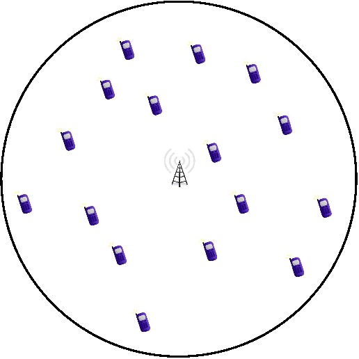
Figure 10: An example of a physical system that “naturally” generates ensembles of sparse ${{A}}$ that SHO-FA can use: Suppose there are ${k}$ cellphones (out of a set of ${n}$ possible different cellphones in the whole world) in a certain neighbourhood that has a base-station. The goal is for the ${j}$-th cellphone to communicate its information ($x_{{j}}$) to the base-station at least once per frame of ${c}{k}$ consecutive time-slots. The challenge is to do so in a distributed manner, since multiple cellphones transmitting at the same time ${i}$ would result in a linear combination $y_{{i}}=\sum_{{j}}a_{{i}{j}}x_{{j}}$ of their transmissions reaching the base-station, where $a_{{i}{j}}$ corresponds to the channel gain from the cellphone ${j}$ to the base-station during time-slot ${i}$. With high probability, such $a_{{i}{j}}$ satisfying the properties we require for our algorithm to work – “sparsity” (relatively few transmitters transmit at any given time) and “distinctness” (with high probability the channel gains from different transmitters are different). Each cellphone transmits $x_{{j}}$ to the base-station a constant (${d}$) number of times in each frame – the set of ${d}$ time-slots in each frame that cellphone ${j}$ transmits in is chosen by ${j}$ uniformly at random from the set of all ${{{c}{k}}\choose{{d}}}$ sets of slots.

While the ensemble of matrices $\{{{A}}\}$ we present above has carefully chosen identification entries, and all the non-zero verification entries have unit magnitude, as noted in Remark 1, the implicit ideas underlying SHO-FA work for significantly more general ensembles of matrices. In particular, Property 1 only requires that the graph $\mathcal{G}$ underling ${{A}}$ be “sparse”, with a constant number of non-zero entries per column. Property 2 only requires that each non-zero entry in each row be distinct – which is guaranteed with high probability, for instance, if each entry is chosen $i.i.d$ from any distribution with sufficiently large support. An example of such a scenario is shown in Figure 10. This naturally motivates the application of SHO-FA to a variety of scenarios, for $\it{e.g.}$, neighbor discovery in wireless communication [40].

III Approximate reconstruction in the presence of noise

A prominent aspect of the design presented in the previous section is that it relies on exact determination of all the phases as well as magnitudes of the measurement vector ${{A}}{\mathbf{x}}$. In practice, however, we often desire that the measurement and reconstruction be robust to corruption both before and and during measurements. In this section, we show that our design may be modified slightly such that with a suitable decoding procedure, the reconstruction is robust to such "noise".

We consider the following setup. Let ${\mathbf{x}}\in{}^{n}$ be a ${k}$-sparse signal with support ${\mathcal{S}}({\mathbf{x}})=\{{j}:x_{{j}}\neq 0\}$. Let ${\mathbf{z}}\in{}^{n}$ have support $\{1,2,\ldots,{n}\}\setminus{\mathcal{S}}({\mathbf{x}})$ with each $z_{j}$ distributed according to a Gaussian distribution with mean $0$ and variance $\sigma_{z}^{2}$. Denote the measurement matrix by ${{A}}\in{}^{{m}\times{n}}$ and the measurement vector by ${\mathbf{y}}\in{}^{m}$. Let ${\mathbf{e}}\in{}^{{m}}$ be the measurement noise with $e_{i}$ distributed as a Complex Gaussian with mean $0$ and variance $\sigma_{e}^{2}$ along each axis. ${\mathbf{y}}$ is related to the signal as

$${\mathbf{y}}={{A}}({\mathbf{x}}+{\mathbf{z}})+{\mathbf{e}}.$$

We first propose a design procedure for ${{A}}$ satisfying the following properties.

Theorem 4.

Let ${k}={\mathcal{O}}({n}^{1-\Delta})$ for some $\Delta>0$. There exists a reconstruction algorithm SHO-FA for ${{A}}\in{}^{{m}\times{n}}$ such that

1. ${m}={c}{k}$

2. SHO-FA consists of at most $4{k}$ iterations, each involving a constant number of arithmetic operations with a precision of ${\mathcal{O}}(\log{{n}})$ bits.

3. With probability $1-o(1/{k})$ over the design of ${{A}}$ and randomness in ${\mathbf{e}}$ and ${\mathbf{z}}$,

   $$||\hat{{\mathbf{x}}}-{\mathbf{x}}||_{1}\leq C\left(||{\mathbf{z}}||_{1}+\sqrt{\log{{k}}}||{\mathbf{e}}||_{1}\right)$$

   for some $C=C(\sigma_{z},\sigma_{e})>0$.

We present a “simple” proof of the above theorem in Sections LABEL:sec:new_ideas to III-C. In Theorem 6, we outline an analysis (based on the work of [37]) that leads to a tighter characterization of the constant factors in the parameters of Theorem 4.

Recall that in the exactly ${k}$-sparse case, the decoding in ${t}$-th iteration relies on first finding an ${\mathcal{S}}{({t})}$-leaf node, then decoding the corresponding signal coordinate and updating the undecoded measurements. In this procedure, it is critical that each iteration operates with low reconstruction errors as an error in an earlier iteration can propagate and cause potentially catastrophic errors. In general, one of the following events may result in any iteration ending with a decoded signal value that is far from the true signal value:

1. The decoder picks an index outside the set $\{{i}:({{A}}{\mathbf{x}})_{{i}}\neq 0\}$, but in the set $\{{i}:({{A}}({\mathbf{x}}+{\mathbf{z}})+{\mathbf{e}})_{{i}}\neq 0\}\}$.

2. The decoder picks an index within the set $\{{i}:({{A}}{\mathbf{x}})_{{i}}\neq 0\}$ that is also a leaf for $\mathcal{S}$ with parent node ${j}$, but the presence of noise results in the decoder identifying (and verifying) a node ${j}^{\prime}\neq{j}$ as the parent and, subsequently, incorrectly decoding the signal at ${j}^{\prime}$.

3. The decoder picks an index within the set $\{{i}:({{A}}{\mathbf{x}})_{{i}}\neq 0\}$ that is not a leaf for $\mathcal{S}$, but the presence of noise results in the decoder identifying (and verifying) a node ${j}$ as the parent and, subsequently, incorrectly decoding the signal at ${j}$.

4. The decoder picks an index within the set $\{{i}:({{A}}{\mathbf{x}})_{{i}}\neq 0\}$ that is a leaf for $\mathcal{S}$ with parent node ${j}$, which it also identifies (and verifies) correctly, but the presence of noise introduces a small error in decoding the signal value. This error may also propagate to the next iteration and act as "noise" for the next iteration.

To overcome these hurdles, our design takes the noise statistics into account to ensure that each iteration is resilient to noise with a high probability. This achieved through several new ideas that are presented in the following for ease of exposition. Next, we perform a careful analysis of the corresponding decoding algorithm and show that under certain regularity conditions, the overall failure probability can be made arbitrarily small to output a reconstruction that is robust to noise. Key to this analysis is bounding the effect of propagation of estimation error as the decoder steps through the iterations.

III-A Key ideas

III-A1 Truncated reconstruction

We observe that in the presence of noise, it is unlikely that signal values whose magnitudes are comparable to that of the noise values can be successfully recovered. Thus, it is futile for the decoder to try to reconstruct these values as long as the overall penalty in $l_{1}$-norm is not high. The following argument shows that this is indeed the case. Let

$${\mathcal{S}}_{\delta}({\mathbf{x}})=\{{j}:|x_{{j}}|<\delta/{k}\}.$$ (2)

and let ${\mathbf{x}}_{{\mathcal{S}}_{\delta}}$ be the vector defined as

$$(x_{{\mathcal{S}}_{\delta}})_{j}=\left\{\begin{array}[]{ll}0&\ {j}\notin{\mathcal{S}}_{\delta}({\mathbf{x}})\\ x_{{j}}&\ {j}\in{\mathcal{S}}_{\delta}({\mathbf{x}}).\end{array}\right.$$

Similarly, define ${\mathbf{x}}_{{\mathcal{S}}_{\delta}^{c}}$ which has non-zero entries only within the set ${\mathcal{S}}({\mathbf{x}})\setminus{\mathcal{S}}_{\delta}({\mathbf{x}})$. The following sequence of inequalities shows that the total $l_{1}$ norm of ${\mathbf{x}}_{S_{\delta}}$ is small:

$$||{\mathbf{x}}_{{\mathcal{S}}_{\delta}}||_{1} = \sum_{{j}\in{\mathcal{S}}_{\delta}({\mathbf{x}})}|x_{j}|$$ (3)

$$\leq |{\mathcal{S}}_{\delta}({\mathbf{x}})|\frac{\delta}{{k}}$$

$$\leq |{\mathcal{S}}({\mathbf{x}})|\frac{\delta}{{k}}$$

$$= \delta.$$

Further, as an application of triangle inequality and the bound in (3), it follows that

$$||\hat{{\mathbf{x}}}-{\mathbf{x}}||_{1} = ||\hat{{\mathbf{x}}}-{\mathbf{x}}_{{\mathcal{S}}_{\delta}^{c}}-{\mathbf{x}}_{{\mathcal{S}}_{\delta}}||_{1}$$ (4)

$$\leq ||\hat{{\mathbf{x}}}-{\mathbf{x}}_{{\mathcal{S}}^{c}_{\delta}}||_{1}+||{\mathbf{x}}_{{\mathcal{S}}_{\delta}}||_{1}$$

$$\leq ||\hat{{\mathbf{x}}}-{\mathbf{x}}_{{\mathcal{S}}^{c}_{\delta}}||_{1}+\delta$$

Keeping the above in mind, we rephrase our reconstruction objective to satisfy the following criterion with a high probability:

$$||\hat{{\mathbf{x}}}-{\mathbf{x}}_{{\mathcal{S}}^{c}_{\delta}}||_{1} \leq C_{1}(||{\mathbf{z}}||_{1}+{k}^{2}||{\mathbf{e}}||_{1}),$$ (5)

while simultaneously ensuring that our choice of parameter $\delta$ satisfies

$$\delta<C_{2}||{\mathbf{z}}||_{1}$$ (6)

for some $C_{2}$, with a high probability.

III-A2 Phase quantization

In the noisy setting, even when ${i}$ is a leaf node for ${\mathcal{S}}({\mathbf{x}})$, the phase of $y_{{i}}$ may differ from the phase assigned by the measurement. This is geometrically shown in Figure 12a for a measurement matrix ${{A}}^{\prime}$. To overcome this, we modify our decoding algorithm to work with "quantized" phases, rather than the actual received phases. The idea behind this is that if ${i}$ is a leaf node for ${\mathcal{S}}({\mathbf{x}})$, then quantizing the phase to one of the values allowed by the measurement identifies the correct phase with a high probability. The following lemma facilitates this simplification.

Lemma 5 (Almost bounded phase noise).

Let ${\mathbf{x}},{\mathbf{z}}\in{}^{{n}}$ with $|x_{{j}}|>\delta/{k}$ for each ${j}$. Let ${{A}}^{\prime}\in{}^{{m}^{\prime}\times{n}}$ be a complex valued measurement matrix with the underlying graph $\mathcal{G}$. Let ${i}$ be a leaf node for ${\mathcal{S}}({\mathbf{x}})$. Let $\Delta\theta_{{i}}=|\angle y_{{i}}-\angle({{A}}^{\prime}{\mathbf{x}})_{{i}}|$. Then, for every $\alpha>0$,

$$E_{{\mathbf{z}},{\mathbf{e}}}\large(\Delta\theta_{{i}}\large)\leq\sqrt{\frac{2\pi{k}^{2}({d}{n}\sigma_{z}^{2}/{c}{k}+\sigma_{e}^{2})}{\delta^{2}}}$$

and

$$\Pr_{{\mathbf{z}},{\mathbf{e}}}\bigg{(}\Delta\theta_{{i}}>\alpha E_{{\mathbf{z}},{\mathbf{e}}}\large(\Delta\theta_{{i}}\large)\bigg{)}<\frac{1}{2}e^{-(\alpha^{2}/2\pi)}.$$

Proof.

See Appendix -E. ■ For a desired error probability $\epsilon^{\prime}$, the above lemma stipulates that it suffices to let $\alpha=\sqrt{2\pi\log(1/2\epsilon^{\prime})}$. We examine the effect of phase noise in more detail in Appendix -F.

III-A3 Repeated measurements

Our algorithm works by performing a series of ${\Gamma}\geq 1$ identification and verification measurements in each iteration instead of a single measurement of each type as done in the exactly ${k}$-sparse case. The idea behind this is that, in the presence of noise, even though a single set of identification and verification measurements cannot exactly identify the coordinate ${j}$ from the observed $y_{i}$, it helps us narrows down the set of coordinates ${j}$ that can possibly contribute to give the observed phase. Performing measurements repeatedly, each time with a different measurement matrix, helps us identify a single ${j}$ with a high probability.

We implement the above idea by first mapping each ${j}\in\{1,2,\ldots,{n}\}$ to its ${\Gamma}$-digit representation in base $\bbg=\{0,1,\ldots\lceil{n}^{1/{\Gamma}}-1\rceil\}$. For each ${j}\in\{1,2,\ldots,{n}\}$, let ${g}({j})=({g}_{1}({j}),{g}_{2}({j}),\ldots,{g}_{\Gamma}({j}))$ be the ${\Gamma}$-digit representation of ${j}$. Next, perform one pair of identification and verification measurements (and corresponding phase reconstructions), each of which is intended to distinguish exactly one of the digits. In our construction, we only need a constant number of such phase measurements per iteration. See Fig 13 for an illustrating example.

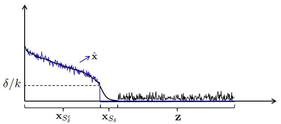
Figure 11: The black curve corresponds to the magnitudes of ${\mathbf{x}}+{\mathbf{z}}$ (for ease of visual presentation, the components of ${\mathbf{x}}$ have been sorted in decreasing order of magnitude and placed in the first ${k}$ components of the signal, but the components of ${\mathbf{z}}$ are unsorted. The blue curve corresponds to our reconstruction $\hat{{\mathbf{x}}}$ of ${\mathbf{x}}$. Note that we only attempt to reconstruct components of ${\mathbf{x}}$ that are “sufficiently large" (that is, we make no guarantees about correct reconstruction of components of ${\mathbf{x}}$ in ${{\mathcal{S}}}_{\delta}({\mathbf{x}})$, , i.e, those components of ${\mathbf{x}}$ that are smaller than some “threshold" $\delta/{k}$. Here $\delta$ is a parameter of code-design to be specified later. As shown in Section III-A1, as long as $\delta$ is not “too large", this relaxation does not violate our relaxed reconstruction criteria (5).

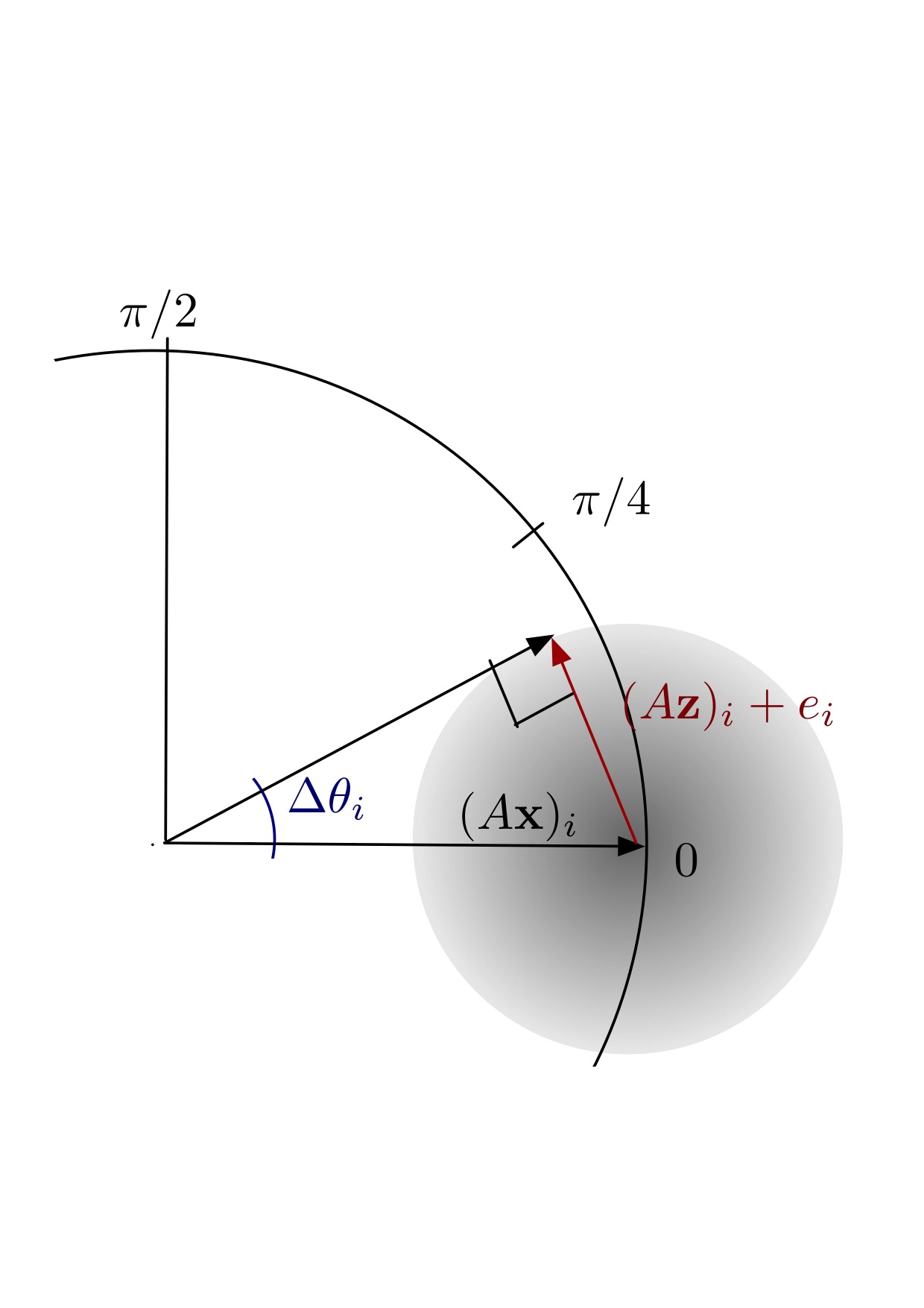
(a) Maximum phase displacement occurs when the contribution due to noise, i.e., $({{A}}{\mathbf{z}})_{i}+e_{i}$ is orthogonal to the measurement ${\mathbf{y}}_{i}$

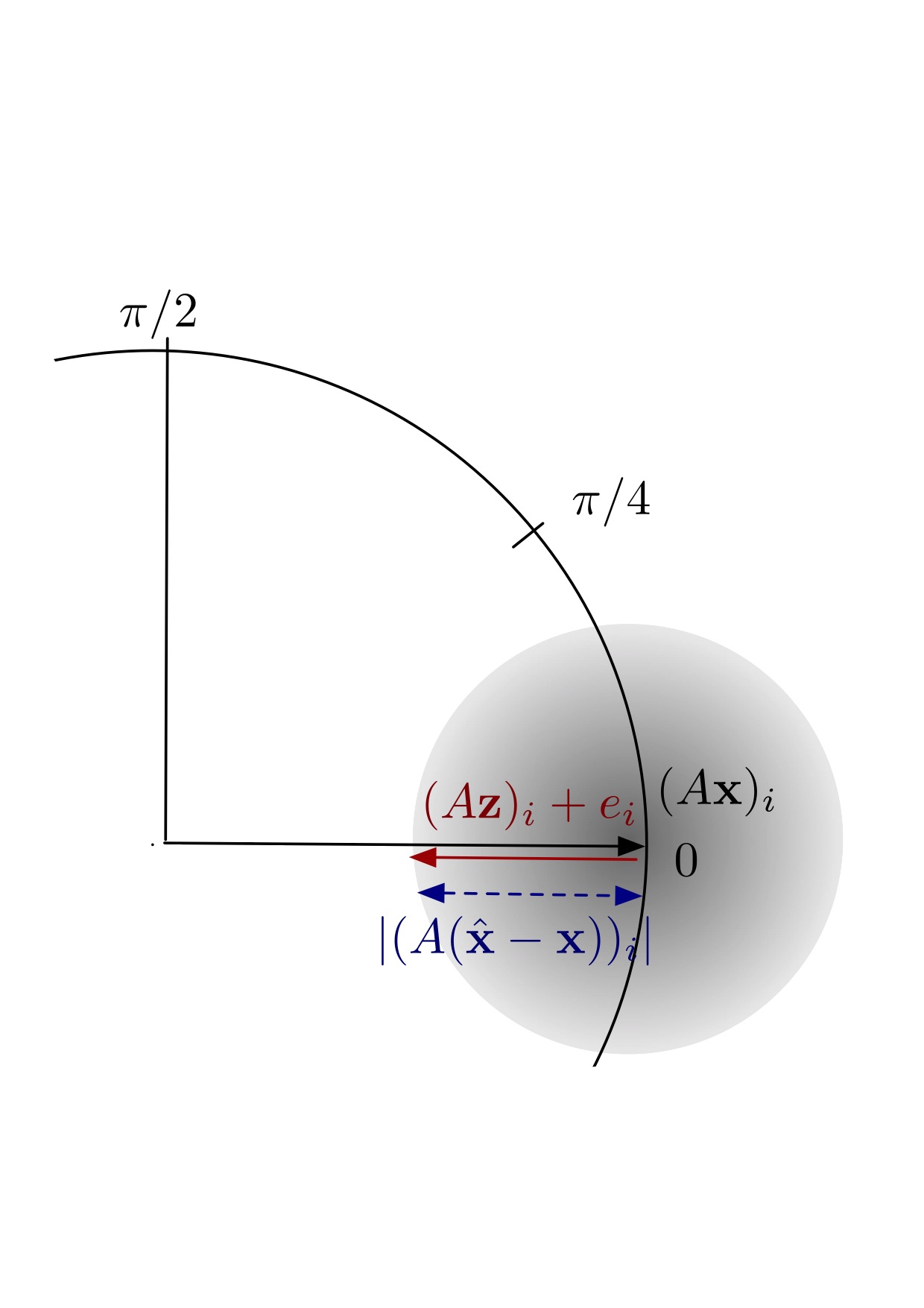
(b) Maximum magnitude displacement takes place when the contribution due to noise is aligned with $({{A}}{\mathbf{x}})_{i}$

Figure 12: The effect of noise on a measurement output

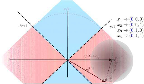
(a) The decoder "randomly" picks $y_{1}$. Since the phase of $y_{1}^{(I,1)}$ is between $-\pi/4$ and $\pi/4$, the decoder can distinguish that the first bit of non-zero location is $0$ since the decoder can tolerate at most $\pi/4$ phase displacement for $y_{1}$. So, the non-zero entry is one of $x_{1}$, $x_{2}$, $x_{3}$, $x_{4}$.

(b) The decoder "randomly" picks $y_{1}$ again. Since the phase of $y_{1}^{(I,2)}$ is between $3\pi/4$ and $5\pi/4$, the decoder can distinguish that the second bit of non-zero location is $1$ since the decoder can tolerate at most $\pi/4$ phase displacement for $y_{1}$. So, the non-zero entry is one of $x_{3}$, $x_{4}$, $x_{7}$, $x_{8}$. Combing the output in the first phase measurement, we conclude that the non-zero entry is one of $x_{3}$ and $x_{4}$.

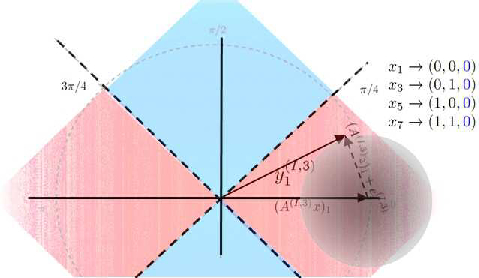
(c) The decoder "randomly" picks $y_{1}$ again. Since the phase of $y_{1}^{(I,3)}$ is between $-\pi/4$ and $\pi/4$, the decoder can distinguish that the third bit of non-zero location is $0$ since the decoder can tolerate at most $\pi/4$ phase displacement for $y_{1}$. So, the non-zero entry is one of $x_{1}$, $x_{3}$, $x_{5}$, $x_{7}$. Combing the outputs in the first and second phase measurement, we conclude that the non-zero entry is $x_{3}$.

Figure 13: If we were to distinguish each ${j}$ from $1$ to $8$ by a different phase, the decoder can tolerate at most $\pi/14$ phase displacement for any output $y_{i}$. Instead, we first represent each ${j}=1,2,\ldots,8$ by a three-length binary vector. Next, we perform three sets of phase assignments – one for each digit. It is easily seen that by allowing multiple measurements, the noise tolerance for the decoder increases.

III-B Measurement Design

As in the exactly ${k}$-sparse case, we start with a randomly drawn left regular bipartite graph $\mathcal{G}$ with ${n}$ nodes on the left and ${m}^{\prime}$ nodes on the right.

Measurement matrix: The measurement matrix ${{A}}\in{}^{2{m}^{\prime}{\Gamma}\times{n}}$ is chosen based on the graph $\mathcal{G}$. The rows of ${{A}}$ are partitioned into ${m}^{\prime}$ groups, with each group consisting of $2{\Gamma}$ consecutive rows. The ${j}$-th entries of the rows $2({i}-1){\Gamma}+1,({i}-1){\Gamma}+2,\ldots,2{i}{\Gamma}$ are denoted by $a^{(I,1)}_{{i},{j}},a^{(I,2)}_{{i},{j}},\ldots,a^{(I,{\Gamma})}_{{i},{j}},a^{(V,1)}_{{i},{j}},a^{(V,2)}_{{i},{j}},\ldots,a^{(V,{\Gamma})}_{{i},{j}}$ respectively. In the above notation, $I$ and $V$ are used to refer to identification and verification measurements.

For ease of notation, for each ${\gamma}=1,2,\ldots,{\Gamma}$, we use ${{A}}^{(I,{\gamma})}$ (resp. ${{A}}^{(V,{\gamma})}$) to denote the sub-matrix of ${{A}}$ whose $({i},{j})$-th entry is $a^{(I,{\gamma})}_{{i},{j}}$ (resp. $a^{(V,{\gamma})}_{{i},{j}}$).

We define the ${\gamma}$-th identification matrix ${{A}}^{(I,{\gamma})}$ as follows. For each $({i},{j})$, if the graph $\mathcal{G}$ does not have an edge connecting ${i}$ on the right to ${j}$ on the left, then $a^{(I,{\gamma})}_{{i},{j}}=0$. Otherwise, we set $a^{(I,{\gamma})}_{{i},{j}}$ to be the unit-norm complex number

$$a^{(I,{\gamma})}_{{i},{j}}=e^{\iota{g}_{\gamma}({j})\pi/2(|\bbg|-1|)}.$$

Note here that the construction for the exactly ${k}$-sparse case can be recovered by setting ${\Gamma}=1$, which results in $\bbg=\{1,2,\ldots,{n}\}$ and ${g}_{\gamma}({j})={j}$.

Next, we define the ${\gamma}$-th verification matrix ${{A}}^{(V,{\gamma})}$ in a way similar to how we defined the verification entries in the exactly ${k}$-sparse case. For each $({i},{j})$, if the graph $\mathcal{G}$ does not have an edge connecting ${i}$ on the right to ${j}$ on the left, then $a^{(V,{\gamma})}_{{i},{j}}=0$. Otherwise, we set

$$a^{(V,{\gamma})}_{{i},{j}}=e^{\iota\theta^{(V,{\gamma})}_{{i}{j}}},$$

where $\theta^{(V,{\gamma})}_{{i},{j}}$ is drawn uniformly at random from $\{0,\pi/2(|\bbg|-1),\pi/(|\bbg|-1),3\pi/2(|\bbg|-1)\ldots,\pi/2\}$.

Given an signal vector ${\mathbf{x}}$, signal noise ${\mathbf{z}}$, and measurement noise ${\mathbf{e}}$, the measurement operation produces a measurement vector ${\mathbf{y}}={{A}}({\mathbf{x}}+{\mathbf{e}})$. Since ${{A}}$ can be partitioned into ${\Gamma}$ identification and ${\Gamma}$ verification rows, we think of the measurement vector ${\mathbf{y}}$ as a collection of outcomes from ${\Gamma}$ successive measurement operations such that

$${\mathbf{y}}^{(I,{\gamma})}=A^{(I,{\gamma})}({\mathbf{x}}+{\mathbf{z}})+{\mathbf{e}}^{(I,{\gamma})}$$

and

$${\mathbf{y}}^{(V,{\gamma})}=A^{(V,{\gamma})}({\mathbf{x}}+{\mathbf{z}})+{\mathbf{e}}^{(V,{\gamma})}$$

are the outcomes from the ${\gamma}$-th measurement and ${\mathbf{y}}=(({\mathbf{y}}^{(I,{\gamma})},{\mathbf{y}}^{(V,{\gamma})}):1\leq{\gamma}\leq{\Gamma})$.

III-C Reconstruction

The decoding algorithm for this case extends the decoding algorithm presented earlier for the exactly ${k}$-sparse case by including the ideas presented in Section III-A. The total number of iterations for our algorithm is upper bounded by $4{k}$.

1. We initialize by setting the signal estimate vector $\hat{{\mathbf{x}}}{(1)}$ to the all-zeros vector $0^{{n}}$, and for each ${\gamma}=1,2,\ldots,{\Gamma}$, we set the residual measurement identification/verification vectors $\tilde{{\mathbf{y}}}^{(I,{\gamma})}(1)$ and $\tilde{{\mathbf{y}}}^{(V,{\gamma})}(1)$ to the decoder’s observations ${\mathbf{y}}^{(I,{\gamma})}$ and ${\mathbf{y}}^{(V,{\gamma})}$.

   Let ${\mathcal{D}}{(1)}$, the initial neighborly set, be the set of indices ${i}$ for which, at which the magnitude corresponding to all verification and identification vectors is greater than $\delta/{k}$, i.e.,

   $${\mathcal{D}}{(1)}=\bigcap_{{\gamma}=1}^{\Gamma}\left\{{i}:|y^{(I,{\gamma})}_{{i}}|>\frac{\delta}{{k}},\ |y^{(V,{\gamma})}_{{i}}|>\frac{\delta}{{k}}\right\}$$

   vector ${\mathbf{y}}^{(V)}$, i.e., the set $\{{i}\leq{m}:\tilde{y}_{{i}}^{(V)}{(1)}\neq 0\}$. This step takes ${\mathcal{O}}({k})$ steps, since merely reading ${\mathbf{y}}$ to check for the zero locations of ${\mathbf{y}}^{(V)}$ takes that long.

2. The ${t}^{th}$ decoding iteration accepts as its input the ${t}^{th}$ signal estimate vector $\hat{{\mathbf{x}}}^{({t})}$, the ${t}^{th}$ neighbourly set ${\mathcal{D}}{{({t})}}$, and the ${t}^{th}$ residual measurement identification/verification vectors $\left((\tilde{{\mathbf{y}}}^{(I,{\gamma})}{({t})},\tilde{{\mathbf{y}}}^{(V,{\gamma})}{({t})}):{\gamma}=1,2,\ldots,{\Gamma}\right)$. In ${\mathcal{O}}(1)$ steps it outputs the $({t}+1)^{th}$ signal estimate vector $\hat{{\mathbf{x}}}^{({t}+1)}$, the $({t}+1)^{th}$ neighbourly set ${\mathcal{D}}{{({t}+1)}}$, and the $({t}+1)^{th}$ residual measurement identification/verification vectors$\left((\tilde{{\mathbf{y}}}^{(I,{\gamma})}{({t}+1)},\tilde{{\mathbf{y}}}^{(V,{\gamma})}{({t}+1)}):{\gamma}=1,2,\ldots,{\Gamma}\right)$ after the performing the following steps sequentially (each of which takes at most a constant number of atomic steps).

3. Pick a random ${i}{({t})}$: The decoder picks ${i}{({t})}$ uniformly at random from ${\mathcal{D}}{({t})}$

4. Compute quantized phases: For each ${\gamma}=1,2,\ldots,{\Gamma}$, compute the current identification angles, $\hat{\theta}^{(I,{\gamma})}_{t}$, and current identification angles, $\hat{\theta}^{(I,{\gamma})}_{t}$ defined as follows:

   $$\hat{\theta}^{(I,{\gamma})}_{t} = \left[\frac{2(|\bbg|-1|)\left(\angle y^{(I,\gamma)}_{{i}{({t})}}(\mbox{mod }\pi)\right)}{\pi}\right]\frac{\pi}{2(|\bbg|-1|)},$$

   $$\hat{\theta}^{(V,{\gamma})}_{t} = \left[\frac{2(|\bbg|-1|)\left(\angle y^{(V,\gamma)}_{{i}{({t})}}(\mbox{mod }\pi)\right)}{\pi}\right]\frac{\pi}{2(|\bbg|-1|)}.$$

   In the above, $[\cdot]$ denotes the closest integer function. Since there are $\Theta({n})$ different phase vectors, to perform this computation, ${\mathcal{O}}(\log{n})$ precision and ${\mathcal{O}}(1)$ steps suffice.

   For each ${\gamma}=1,2,\ldots,{\Gamma}$, let $\hat{{g}}_{{\gamma}}^{({t})}=2(|\bbg|-1|)\hat{\theta}^{(I,{\gamma})}/\pi$ be the current estimate of ${\gamma}$-th digit and let ${j}{({t})}$ be the number whose representation in is $(\hat{{g}}_{1}^{({t})},\hat{{g}}_{2}^{({t})},\ldots,\hat{{g}}_{{\Gamma}}^{({t})})$.

5. Check if the current identification and verification angles correspond to a valid and unique j: This step determines if ${i}{({t})}$ is a leaf node for ${\mathcal{S}}_{\delta}({\mathbf{x}}-\hat{{\mathbf{x}}}{({t})})$. This operation is similar to the corresponding exact-${k}$ case. The main difference here is that we perform the verification operation on each of the ${\Gamma}$ measurements separately and declare ${i}{({t})}$ as a leaf node only if it passes all the verification tests. The verification step for the ${\gamma}$-th measurement is given by the test:

   $$\hat{\theta}^{(V,{\gamma})}_{t}\overset{?}{=}\theta_{{i}{({t})},{j}{({t})}}^{(V,{\gamma})}.$$

   If the above test succeeds for every ${\gamma}=1,2,\ldots,{\Gamma}$, we set $\Delta x{({t})}$ to $|\tilde{y}^{(I,\gamma)}_{{i}{({t})}}({t})|$ if $\angle y^{(I,\gamma)}_{{i}{({t})}}\in(-\pi/4,3\pi/4]$, and $-|\tilde{y}^{(I,\gamma)}_{{i}{({t})}}({t})|$ if $\angle y^{(I,\gamma)}_{{i}{({t})}}\in(3\pi/4,7\pi/4]$ Otherwise, we set $\Delta x{({t})}=0$. This step requires at most ${\Gamma}$ verification steps and therefore, can be completed in ${\mathcal{O}}(1)$ steps.

6. Update $\hat{{\mathbf{x}}}{({t}+1)}$, $\tilde{{\mathbf{y}}}{({t}+1)}$, and ${\mathcal{D}}{({t}+1)}$: If the verification tests in the previous steps failed, there are no updates to be done, i.e., set $\hat{{\mathbf{x}}}{({t}+1)}=\hat{{\mathbf{x}}}{({t})}$, $\tilde{{\mathbf{y}}}{({t}+1)}=\tilde{{\mathbf{y}}}{({t})}$, and ${\mathcal{D}}{({t}+1)}={\mathcal{D}}{({t})}$.

   Otherwise, we first update the current signal estimate to $\hat{{\mathbf{x}}}{({t}+1)}$ by setting the ${j}{({t})}$-th coordinate to $\Delta x{({t})}$. Next, let ${i}_{1},{i}_{2},{i}_{3}$ be the possible neighbours of ${j}{({t})}$. We compute the residual identification/verification vectors $\tilde{{\mathbf{y}}}{({t}+1)}$ at ${i}_{1},{i}_{2},{i}_{3}$ by subtracting the weight due to $\Delta x{({t})}$ at each of them. Finally, we update the neighbourly set by removing ${i}_{1},{i}_{2}$, and ${i}_{3}$ from ${\mathcal{D}}{({t})}$ to obtain ${\mathcal{D}}{({t}+1)}$.

The decoding algorithm terminates after the $T$-th iteration, where $T=\min\{4{k},\{{t}:{\mathcal{D}}{({t}+1)}=\phi\}\}$.

III-D Improving performance guarantees of SHO-FA via Set-Query Algorithm of [37]

In [37], Price considers a related problem called the Set-Query problem. In this setup, we are given an unknown signal vector ${\mathbf{x}}$ and the objective is to design a measurement matrix ${{A}}$ such that given ${\mathbf{y}}={{A}}{\mathbf{x}}+{\mathbf{e}}$ (here, ${\mathbf{e}}$ is an arbitrary “noise” vector), and a desired query set ${\mathcal{S}}\subseteq\{1,2,\ldots,{n}\}$, the decoder outputs a reconstruction $\hat{{\mathbf{x}}}$ with having support ${\mathcal{S}}$ such that $\hat{{\mathbf{x}}}-{\mathbf{x}}_{\mathcal{S}}$ is “small”. The following Theorem from [37] states the performance guarantees for a randomised construction of ${{A}}$.

Theorem 5 (Theorem 3.1 of [37]).

For every $\epsilon>0$, there is a randomized sparse binary sketch matrix $A$ and recovery algorithm $\mathscr{A}$, such that for any ${\mathbf{x}}\in\mathbb{R}^{n}$, ${\mathcal{S}}\subseteq\{1,2,\ldots,{n}\}$ with $|{\mathcal{S}}|={k}$, $\hat{{\mathbf{x}}}=\mathscr{A}({{A}}{\mathbf{x}}+{\mathbf{e}},{\mathcal{S}})\in\mathbb{R}^{n}$ has support ${\mathcal{S}}(\hat{{\mathbf{x}}})\subseteq{\mathcal{S}}$ and

$$||\hat{{\mathbf{x}}}-{\mathbf{x}}_{\mathcal{S}}||_{l}\leq(1+\epsilon)(||{\mathbf{x}}-{\mathbf{x}}_{\mathcal{S}}||_{l}+||{\mathbf{e}}||_{l})$$

for each $l\in\{1,2\}$ with probability at least $1-1/{k}$. ${{A}}$ has ${\mathcal{O}}({k})$ rows and $\mathscr{A}$ runs in ${\mathcal{O}}({k})$ time.

We argue that the above design may be used in conjunction with our SHO-FA algorithm from Theorem  4 to give stronger reconstruction guarantee than Theorem 4. In fact, this allows us to even prove a stronger reconstruction guarantee of $\ell_{2}<\ell_{2}$ form. The following theorem makes this precise.

Theorem 6.

Let ${k}={\mathcal{O}}({n}^{1-\Delta})$ for some $\Delta>0$ and let $\epsilon>0$. There exists a reconstruction algorithm SHO-FA-NO for ${{A}}\in{}^{{m}\times{n}}$ such that

1. ${m}={c}{k}$

2. SHO-FA-NO consists of at most $5{k}$ iterations, each involving a constant number of arithmetic operations with a precision of ${\mathcal{O}}(\log{{n}})$ bits.

3. With probability $1-o(1/{k})$ over the design of ${{A}}$ and randomness in ${\mathbf{e}}$ and ${\mathbf{z}}$, and for each $l\in\{1,2\}$,

   $$||\hat{{\mathbf{x}}}-{\mathbf{x}}||_{l}\leq(1+\epsilon)\left(||{\mathbf{z}}||_{l}+||{\mathbf{e}}||_{l}\right).$$

Proof.

We first note that the measurement matrix proposed in [37] is independent of the query set ${\mathcal{S}}$ and depends only on the size ${k}$ of the set ${\mathcal{S}}$. We design our measurement matrix ${{A}}\in\mathbb{R}^{{m}\times{n}}$ by combining the measurement matrices from Theorem 4 and Theorem 5 as follows. Let ${{A}}_{1}\in\mathbb{R}^{{m}_{1}\times{n}}$ be drawn according to Theorem 4 and ${{A}}_{2}\in\mathbb{R}^{{m}_{2}\times{n}}$ be drawn according to Theorem 5 for some ${m}_{1}$ and ${m}_{2}$ scaling as ${\mathcal{O}}({k})$ so as to achieve an error probability ${\mathcal{O}}(1/{k})$. Let ${{A}}\in\mathbb{R}^{{m}\times{n}}$ with ${m}={m}_{1}+{m}_{2}$ with the upper ${m}_{1}$ rows consisting of all rows of ${{A}}_{1}$ and the lower ${m}_{2}$ rows consisting of all the row of ${{A}}_{2}$.

To perform the decoding, the decoder first produces a coarse reconstruction $\hat{\tilde{{\mathbf{x}}}}$ by passing the first ${m}_{1}$ rows of the measurement output ${\mathbf{y}}$ through the SHO-FA decoding algorithm. Let $\delta$ be the truncation threshold for the decoder. Next, the decoder computes ${\mathcal{S}}_{\delta}({\mathbf{x}})$ to be the support of $\hat{\tilde{{\mathbf{x}}}}$. Finally, the decoder we apply the set query algorithm from 5 with inputs $\left([y_{{m}_{1}+2},\ldots,y_{{m}_{2}}]^{T},{\mathcal{S}}_{\delta}({\mathbf{x}})\right)$ to obtain a reconstruction $\hat{{\mathbf{x}}}$ that satisfies the desired reconstruction criteria.

■

IV SHO-FA with Integer-valued measurement matrices (SHO-FA-INT)

In the measurement designs presented in Sections II and III, a key requirement is that the entries of the measurement matrix may be chosen to be arbitrary real or complex numbers of magnitude (upto ${\mathcal{O}}(\log{n})$ bits of precision). However, in several scenarios of interest, the entries of the measurement matrix are constrained by the measurement process.

• In network tomography [41], one attempts to infer individual link delays by sending test packets along pre-assigned paths. In this case, the overall end-to-end path delay is the sum of the individual path delays along that path, corresponding to a measurement matrix with only $0$s and $1$s (or in general, with positive integers, if loops are allowed).

• If transmitters in a wireless setting are constrained to transmit symbols from a fixed constellation, then the entries of the measurement matrix can only be chosen from a finite ensemble.

In both these examples, the entries of the measurement matrix are tightly constrained.

In this section, we discuss how key ideas from Sections II and III may be applied in compressive sensing problems where the entries of measurement matrix is constrained to take values form a discrete set. For simplicity, we assume that the entries of the matrix ${{A}}$ can take values in the set $\left\{1,2,\ldots,M\right\}$ for some integer $M\in{}^{+}$. For simplicity, we consider only the exact ${k}$-sparse problem, noting that extensions to the approximate ${k}$-sparse case follow from techniques similar to those used in Section III.

IV-A Measurement Design

As in the exactly ${k}$-sparse and approximately sparse cases, the ${\it{measurement}}$ ${\it{matrix}}$ $A$ is chosen based on the structure of $\mathcal{G}$ with ${n}$ nodes on the left and ${m}^{\prime}$ nodes on the right. Each left node has degree equal ${d}$. We denote the edge set by $\mathcal{E}$.

We give a combinatorial construction of measurement matrices that ensure the equivalent of Property 2 in this setting. Let $\zeta(\cdot)$ denote the Riemann-zeta function and let $R\leq\log{({d}{n}/2)}/\log M$ be an integer. We design a $2R{m}^{\prime}\times{n}$ measurement matrix $A$ as follows. First, we partition the rows of ${{A}}$ into ${m}$’ groups of rows, each consisting of $2R$ consecutive rows as follows.

$$A=\left[\begin{array}[]{c:c:c:c}a^{(1)}_{11}&a^{(1)}_{12}&\dots&a^{(1)}_{1{n}}\\ \vdots&\vdots&\ddots&\vdots\\ a^{(R)}_{11}&a^{(R)}_{12}&\dots&a^{(R)}_{2{n}}\\ \hdashline a^{(1)}_{21}&a^{(1)}_{22}&\dots&a^{(1)}_{2{n}}\\ \vdots&\vdots&\ddots&\vdots\\ a^{(R)}_{21}&a^{(R)}_{22}&\dots&a^{(R)}_{2{n}}\\ \hdashline\vdots&\vdots&\ddots&\vdots\end{array}\right]$$

Let the $r$-th and $r+R$-th rows in the ${j}$-th column of the ${i}$-th group of ${{A}}$ are respectively denoted $a_{{i}{j}}^{(I,r)}$ and $a_{{i}{j}}^{(V,r)}$ . Let $a_{{i}{j}}=[a_{{i}{j}}^{(I)}a_{{i}{j}}^{(V)}]=[a_{{i}{j}}^{(I,1)}a_{{i}{j}}^{(I,2)}\ldots a_{{i}{j}}^{(V,R-1)}a_{{i}{j}}^{(V,R)}]^{T}$. First, for each $({i},{j})\notin\mathcal{E}$, we set $a_{{i}{j}}=0$. Next, set the non-zero entries of ${{A}}$ by picking the vectors $(a_{{i}{j}}^{(V)}:({i},{j})\in\mathcal{E})$ by uniformly sampling without replacement from the set

$$\mathcal{C}\triangleq\left\{[c_{1},c_{2},\ldots,c_{R}]^{T}\in[M]^{R}:\mbox{gcd}(c_{1},c_{2},\ldots,c_{R})=1\right\}.$$

Lemma 6 shows that, $M^{R}/2\leq|\mathcal{C}|\leq M^{R}$ (here, $\zeta(\cdot)$ is the Reimann zeta function). Therefore, it suffices that $|\mathcal{E}|\leq M^{R}/\zeta(R)$ for such a sampling to be possible. Further, noting that $|\mathcal{E}|={d}{n}$, $\zeta(R)\leq 2$ (via standard bounds), and $R\leq\log{(dn/2)}/\log{M}$ (by assumption), this condition is satisfied.

Lemma 6.

For $M$ large enough, $M^{R}/2\leq|\mathcal{C}|\leq M^{R}$.

Proof.

The upper bound on $|\mathcal{C}|$ is trivial, since each element of ${\cal C}$ is an $R$ length vector whose each coordinate takes values from the set $[M]$. To prove the lower bound, note that a sufficient condition for $\mbox{gcd}(c_{1},c_{2},\ldots,c_{R})$ to be true is that for each prime number $p\in\bbn$, there exists at least one index $r\in[R]$ such that $p$ does not divide $c_{r}$. Since the number of vectors $(c_{1},c_{2},\ldots,c_{R})\in[M]^{R}$ such that for each $r$, $c_{r}$ is divisible by $p$ is at most $(M/p)^{R}$, the number of vectors in $[M]^{R}$ such that at least one component is not divisible by $p$ is at least $M^{R}(1-p^{-R})$. Denoting the set of prime numbers by $\mathbb{P}$ and extending the above argument to exclude all vectors that are divisible by some prime number greater than or equal to two, we obtain, for $M$ large enough,

$$|{\cal C}|\geq M^{R}\prod_{p:p\in\mathbb{P}}(1-1/p^{-R})=M^{R}/\zeta(R).$$

In the above, the second equality follows from Euler’s product formula for the Reimann zeta function. ■

Pick the vectors $(a_{{i}{j}}^{(I)}:({i},{j})\in\mathcal{E})$ in the following way. First, calculate the “normalized” version of every vector $c$ in ${\cal C}$ by set $nor(c)=c/c_{1}$. Then, rearrange the “normalized” vectors in “lexicographical” order. Finally, assign the original value of $j$-th “normalized” vector to $a_{{i}{j}}^{(I)}$ .

The output of the measurement is a $2R{m}^{\prime}$-length vector ${\mathbf{y}}={{A}}{\mathbf{x}}$. Again, we partition ${\mathbf{y}}$ into ${m}^{\prime}$ groups of $2R$ consecutive rows each, and denote the ${i}$-th sub-vector as $y_{{i}}=[y_{{i}}^{(I)T},y_{{i}}^{(V)T}]^{T}$.

IV-B Reconstruction

The decoding algorithm is conceptually similar to the decoding algorithm presented in Section II-D1. The decoder first generates a list of leaf nodes. Next, it proceeds iteratively by decoding the input value corresponding to one leaf node, and updating the list of leaf nodes by subtracting the contribution of the last decoded signal coordinate from the measurement vector.

Our algorithm proceeds iteratively, and has at most ${k}$ overall number of iterations, with ${t}$ being the variable indexing the iteration number.

1. Initialization: We initialize by setting the signal estimate vector $\hat{{\mathbf{x}}}{(1)}$ to the all-zeros vector $0^{{n}}$, and the residual measurement identification/verification vectors $\tilde{{\mathbf{y}}}^{(I)}(1)$ and $\tilde{{\mathbf{y}}}^{(V)}(1)$ to the decoder’s observations ${\mathbf{y}}^{(I)}$ and ${\mathbf{y}}^{(V)}$.

2. Leaf-Node List: Let $\mathcal{L}(1)$, the initial ${\mathcal{S}}({\mathbf{x}})$-leaf node set, be the set of indices ${i}$ which are ${\mathcal{S}}({\mathbf{x}})$-leaf nodes. We make the list in the following steps:

   1. Compute “normalized” vectors $nor^{(I)}({i})$ and $nor^{(V)}({i})$: Let the “normalized” identification and verification vectors be defined respectively for index $i$ (starting from 1), as follows:

      $$nor^{(I)}({i}) \triangleq \tilde{y}_{{i}}^{(I)}(1)/\tilde{y}_{{i}}^{(I,1)}(1),$$

      $$nor^{(V)}({i}) \triangleq \tilde{y}_{{i}}^{(V)}(1)/\tilde{y}_{{i}}^{(V,1)}(1).$$

   2. Check if the current “normalized” identification and verification vectors correspond to a valid and unique $x_{{j}}$: For this, we check at most two things.

      1. First, we check if $nor^{(I)}({i})$ corresponds ${j}$-th “normalized” $c$, and the corresponding ${j}^{th}$ column of the ${i}^{th}$ group is non-zero. If so, we have “tentatively identified” that the ${i}^{th}$ component of $\tilde{{\mathbf{y}}}$ is a leaf-node of the currently unidentified non-zero components of ${\mathbf{x}}$, and in particular is connected to the ${j}^{th}$ node on the left, and the algorithm proceeds to the next step below. If not, we simply increment ${i}$ by $1$ and return to Step (2a).

      2. Next, we verify our estimate from the previous step. If $nor(a_{{i},{j}}^{(V)})=nor({i})$, the verification test passes, and include ${i}$ in $\mathcal{L}(1)$. If not, we simply increment ${i}$ by $1$ and return to Step (2a).

3. Operations in ${t}^{th}$ iteration:The ${t}^{th}$ decoding iteration accepts as its input the ${t}^{th}$ signal estimate vector $\hat{{\mathbf{x}}}{({t})}$, the ${t}^{th}$ leaf node set $\mathcal{L}({t})$, and the ${t}^{th}$ residual measurement identification/verification vectors $(\tilde{{\mathbf{y}}}^{(I)}{({t})},\tilde{{\mathbf{y}}}^{(V)}{({t})})$. In ${\mathcal{O}}(1)$ steps it outputs the $({t}+1)^{th}$ signal estimate vector $\hat{{\mathbf{x}}}{({t}+1)}$, the $({t}+1^{th}$ leaf node set $\mathcal{L}({t}+1)$, and the $({t}+1)^{th}$ residual measurement identification/verification vectors $(\tilde{{\mathbf{y}}}^{(I)}{({t}+1)},\tilde{{\mathbf{y}}}^{(V)}{({t}+1)})$ after the performing the following steps sequentially (each of which takes at most a constant number of atomic steps):

   1. Pick a random ${i}{({t})}\in\mathcal{L}({t})$: The decoder picks an element ${i}{({t})}$ uniformly at random from the ${t}^{th}$ leaf-node list $\mathcal{L}({t})$.

   2. Compute “normalized” vectors $nor^{(I)}({{t}})$ and $nor^{(V)}({{t}})$: Let the current “normalized” identification and verification vectors be defined respectively as the phases of the residual identification and verification entries being considered in that step, as follows:

      $$nor^{(I)}({t}) \triangleq \tilde{y}_{i{({t})}}^{(I)}{({t})}/\tilde{y}_{i{({t})}}^{(I,1)}{({t})},$$

      $$nor^{(V)}({t}) \triangleq \tilde{y}_{i{({t})}}^{(V)}{({t})}/\tilde{y}_{i{({t})}}^{(V,1)}{({t})}.$$

   3. Locate non-zero entry ${j}$ and derive the value of $\hat{x}_{{j}{({t})}}{({t})}$: For this, we do at most two things.

      1. First, we check if $nor^{(I)}({t})$ corresponds ${j}{({t})}$-th “normalized” $c$. We have identified that the ${i}^{th}$ component of $\tilde{{\mathbf{y}}}$ is a leaf-node of the currently unidentified non-zero components of ${\mathbf{x}}$, and in particular is connected to the ${j}{({t})}^{th}$ node on the left, and the algorithm proceeds to the next step below.

      2. Next, we assign the value, $\tilde{y}_{i{({t})}}^{(I)}{({t})}/a_{{i}{({t})},{j}{({t})}}^{(I)}=\tilde{y}_{i{({t})}}^{(V)}{({t})}/a_{{i}{({t})},{j}{({t})}}^{(V)}$, to $\hat{x}_{{j}{({t})}}{({t})}$ and proceeds the algorithm to the next step below.

   4. Update $\hat{{\mathbf{x}}}{({t}+1)}$, $\mathcal{L}(t+1)$ ,$\tilde{{\mathbf{y}}}^{(I)}{({t}+1)}$, and $\tilde{{\mathbf{y}}}^{(V)}{({t}+1)}$: In particular, at most $7$ components of each of these vectors need to be updated. Specifically, $\hat{x}_{{j}{({t})}}{({t}+1)}$ equals $\tilde{y}_{i{({t})}}^{(I)}{({t})}/a_{{i}{({t})},{j}{({t})}}^{(I)}$. ${i}{({t})}$ is removed from the leaf node set $\mathcal{L}(t)$ and check whether the neighbours of $\hat{x}_{{j}{({t})}}{({t})}$ become leaf node to get the leaf-node list $\mathcal{L}(t+1)$. And finally values each of $\tilde{{\mathbf{y}}}^{(I)}{({t}+1)}$ and $\tilde{{\mathbf{y}}}^{(V)}{({t}+1)}$ are updated from those of $\tilde{{\mathbf{y}}}^{(I)}{({t})}$ and $\tilde{{\mathbf{y}}}^{(V)}{({t})}$ (those corresponding to the neighbours of $\hat{x}_{{j}{({t})}}{({t})}$) by subtracting out $\hat{x}_{{j}{({t})}}{({t})}$ multiplied by the appropriate coefficients of ${{A}}$.

4. Termination: The algorithm stops when the leaf node set is empty, and outputs the last $\hat{{\mathbf{x}}}({t})$.

IV-C Correctness

We show that the algorithm presented above correctly reconstructs the vector ${\hat{{\mathbf{x}}}}$ with a high probability over the random selection of graph $\mathcal{G}$ and the random choice of ${{A}}$ provided that the number of measurements is $\Omega({k}\log{{n}}/\log{M})$

Theorem 7.

Let $\mathcal{G}$ and ${{A}}$ be determined as above. Then, given ${\mathbf{y}}={{A}}{\mathbf{x}}$, SHO-FA-INT outputs a reconstruction ${\hat{{\mathbf{x}}}}$ such that $\Pr_{\mathcal{G},{{A}}}({\hat{{\mathbf{x}}}}\neq{\mathbf{x}})={\mathcal{O}}(1/{k})$. Further, SHO-FA-INT stops in at most ${k}$ iterations and the overall complexity of decoding is ${\mathcal{O}}({k}\log{{n}})$.

Proof.

By definition, the probability that $S({\mathbf{x}})$ and all its subsets expand by at least $(1-\epsilon)$ is at least $1-\alpha$. Therefore, to show that the overall error probability is upper bounded by $2\alpha$, it suffices to show that conditioned on the even that $S({\mathbf{x}})$ and all its subsets expand, the error probability is at most $\alpha$. In particular, noting that each iteration that results in a successful leaf identification decreases the number of undecoded non-zero values by $1$, it suffices to show the following:
a 1) In each iteration ${t}$, ${i}({t})$ is correctly identified as a leaf or non-leaf with probability $1-o(1/{k})$.
a 2) The probability of picking a leaf in each iteration is lower bounded by a constant.
Since we choose the measurement weights $a_{{i}e}$’s for each $e\in E$ and $i\in[{m}]$ to be distinct elements from $\cal C$ by sampling uniformly without replacement, when a node ${i}({t})$ is a leaf node, its parent node $e$ is correctly identified since the measurement vector at node ${i}({t})$ equals $x_{e}a_{{i}({t})e}$. On the other hand, when ${i}({t})$ is not a leaf node, an error might occur if for the specific vector ${\mathbf{x}}$, the measurement output at $y_{i}$ is proportional to the measurement weight for some $e^{\prime\prime}$ connected to ${i}$, $\it{i.e.}$,

$$\sum_{e^{\prime}\in N({i})}x_{e^{\prime}}a_{{i}({t})e^{\prime}}=x^{\prime\prime}a_{{i}({t})e^{\prime\prime}}$$

for some $d^{\prime\prime}$. Since all the measurement weights are chosen randomly, by the Schwartz-Zippel lemma [53, 54], the probability of this event is ${\mathcal{O}}(1/{n})$, which is $o(1/{k})$.

IV-D Decoding complexity

Since there are at most ${k}$ non-zero $x_{e}$’s, the algorithm terminates in ${k}$ steps. Finally, to compute the decoding complexity, note that all arithmetic operations are over vectors in $[M]^{R}$. Therefore, each such operation can be done in ${\mathcal{O}}(R\log M)$ time. Note that $M^{R}={\mathcal{O}}({n})$ by our design choice. Further, the total number of update operations is upper bounded by the number of edges in $\mathcal{E}(S({\mathbf{x}}))$, which is ${\mathcal{O}}({m})$ by the expansion property. Thus, the complexity required by the decoder is ${\mathcal{O}}({k}\log{n})$ or ${\mathcal{O}}({k}(\log{n}+RP))$ if $\hat{\mathbf{x}}$ equal ${\mathbf{x}}$ upto $P$ bits of precision. ■

V Conclusion

In this work we present a suite of algorithms (that we call SHO-FA) for compressive sensing that require an information-theoretically order-optimal number of measurements, bits over all measurements, and encoding, update, and decoding time-complexities. As a bonus, with non-zero probability it can also handle “data-base queries”. The algorithms are robust to noisy signal tails and noisy measurements. The algorithms are “practical” (all constant factors involved are “small”), as validated by both our analysis, and simulations. Our algorithms can reconstruct signals that are sparse in any basis that is known a priori to both the encoder and decoder, and work for “many” ensembles of “sparse” measurement matrices.

-A Proof of Lemma 1

Proof.

It suffices to prove the desired property for all ${\mathcal{S}}({\mathbf{x}})$ of size exactly ${k}$. Let ${\mathcal{S}}^{\prime}({\mathbf{x}})\subseteq{\mathcal{S}}({\mathbf{x}})$. Let $\{(s_{1},t_{1}),(s_{2},t_{2}),\ldots,(s_{{d}|{\mathcal{S}}^{\prime}({\mathbf{x}})|},t_{{d}|{\mathcal{S}}^{\prime}({\mathbf{x}})|})\}$ be the set of outgoing edges from ${\mathcal{S}}^{\prime}({\mathbf{x}})$. Without loss of generality, we assume these edges are drawn in the following manner.

In the initialization stage, we “split” every node on the right of $\mathcal{G}$ to ${d}{n}/{c}{k}$ “virtual” nodes. Each virtual node represents a “true” node on the right. We maintain a set of “remaining” virtual nodes, which we will select and remove virtual nodes from.

To draw the edges, we visit the nodes in ${\mathcal{S}}^{\prime}({\mathbf{x}})$ (on the left of $\mathcal{G}$) sequently. For each node, we select uniformly at random a set of ${d}$ distinct virtual nodes from the remaining virtual node set. We form ${d}$ edges by connecting this node in ${\mathcal{S}}^{\prime}({\mathbf{x}})$ and the true nodes on the right that those ${d}$ selected virtual nodes represent. After the ${d}$ edges are formed, we remove the ${d}$ selected virtual nodes from the remaining virtual node set, and proceed to the next node in ${\mathcal{S}}^{\prime}({\mathbf{x}})$.

In this way, we generate a bipartite graph that is both ${d}$ left-regular and ${d}{n}/{c}{k}$ right-regular; that is, each node on the left has a degree of ${d}$ and each node on the right has a degree of ${d}{n}/{c}{k}$. By using standard arguments of sequential implementation of random experiments, one can verify that the graph generated in this way is chosen uniformly at random from all bipartite graphs that are both ${d}$ left-regular and ${d}{n}/{c}{k}$ right-regular.

For each $i=1,2,\ldots,{d}|{\mathcal{S}}^{\prime}({\mathbf{x}})|$, the probability that the edge $(s_{i},t_{i})$ reaches an “old” true node (on the right) that is already reached by those edges generated ahead of $(s_{i},t_{i})$ is upper bounded as

$$\Pr_{\mathcal{G}}(t_{i}\in\{t_{1},\ldots t_{i-1}\}) \leq \frac{(i-1)}{{c}{k}}$$

$$\leq \frac{{d}|{\mathcal{S}}^{\prime}({\mathbf{x}})|}{{c}{k}}.$$

Let $N({\mathcal{S}}^{\prime}({\mathbf{x}}))$ be the set of all neighboring nodes of the nodes in ${\mathcal{S}}^{\prime}({\mathbf{x}})$. The size of $N({\mathcal{S}}^{\prime}({\mathbf{x}}))$ is no more than $2{d}|{\mathcal{S}}^{\prime}({\mathbf{x}})|/3$ if and only if out of ${d}|{\mathcal{S}}^{\prime}({\mathbf{x}})|$ edges, there exists a set of at least ${d}|{\mathcal{S}}^{\prime}({\mathbf{x}})|/3$ edges fail to reach “new” nodes (on the right). Exploiting this observation, we have

$$\Pr_{\mathcal{G}}\left(|N({\mathcal{S}}^{\prime}({\mathbf{x}}))|\leq 2{d}|{\mathcal{S}}^{\prime}({\mathbf{x}})|/3\right)$$

$$= \Pr_{\mathcal{G}}\left(\bigcup_{\begin{subarray}{c}\sigma\subseteq\{1,\ldots,{d}|{\mathcal{S}}^{\prime}({\mathbf{x}})|\}\\ |\sigma|\geq|{d}{\mathcal{S}}^{\prime}({\mathbf{x}})/3|\end{subarray}}\bigcap_{i\in\sigma}\{t_{i}\in\{t_{1},\ldots t_{i-1}\}\}\right)$$

$$= \Pr_{\mathcal{G}}\left(\bigcup_{\begin{subarray}{c}\sigma\subseteq\{1,\ldots,{d}|{\mathcal{S}}^{\prime}({\mathbf{x}})|\}\\ |\sigma|={d}|{\mathcal{S}}^{\prime}({\mathbf{x}})|/3\end{subarray}}\bigcup_{\sigma^{\prime}\supseteq\sigma}\bigcap_{i\in\sigma^{\prime}}\left\{t_{i}\in\{t_{1},\ldots t_{i-1}\right\}\}\right)$$

$$\leq {{d}|{\mathcal{S}}^{\prime}({\mathbf{x}})|\choose{d}|{\mathcal{S}}^{\prime}({\mathbf{x}})|/3}\Big{(}\frac{{d}|{\mathcal{S}}^{\prime}({\mathbf{x}})|}{{c}{k}}\Big{)}^{{d}|{\mathcal{S}}^{\prime}({\mathbf{x}})|/3}.$$

Consequently, the probability that there exists one ${\mathcal{S}}^{\prime}({\mathbf{x}})\subseteq{\mathcal{S}}({\mathbf{x}})$ so that $|N({\mathcal{S}}^{\prime}({\mathbf{x}}))|\leq 2{d}|{\mathcal{S}}^{\prime}({\mathbf{x}})|/3$ can be bounded by

$$\Pr_{\mathcal{G}}\large(\cup_{{\mathcal{S}}^{\prime}({\mathbf{x}})\subseteq{\mathcal{S}}({\mathbf{x}})}\{|N({\mathcal{S}}^{\prime}({\mathbf{x}}))|\leq 2|{\mathcal{S}}^{\prime}({\mathbf{x}})|\}\large)$$

$$\leq \sum_{{\mathcal{S}}^{\prime}({\mathbf{x}})\subseteq{\mathcal{S}}({\mathbf{x}})}{{d}|{\mathcal{S}}^{\prime}({\mathbf{x}})|\choose{d}|{\mathcal{S}}^{\prime}({\mathbf{x}})|/3}\Big{(}\frac{{d}|{\mathcal{S}}^{\prime}({\mathbf{x}})|}{{c}{k}}\Big{)}^{{d}|{\mathcal{S}}^{\prime}({\mathbf{x}})|/3}$$

$$= \sum_{j=1}^{{k}}{{k}\choose j}{{d}j\choose{d}j/3}\Big{(}\frac{{d}j}{{c}{k}}\Big{)}^{{d}j/3}$$

$$\leq \sum_{j=1}^{{k}}\Big{(}\frac{{k}e}{j}\Big{)}^{j}\big{(}3e\big{)}^{{d}j/3}\Big{(}\frac{{d}j}{{c}{k}}\Big{)}^{{d}j/3}$$

$$= \sum_{j=1}^{k}\Bigg{(}\frac{{k}e}{j}\left(\frac{3{d}je}{{c}{k}}\right)^{{d}/3}\Bigg{)}^{j}$$

$$\leq \sum_{j=1}^{\lceil\sqrt{{k}}\rceil}\Bigg{(}\frac{{k}e}{j}\left(\frac{3{d}je}{{c}{k}}\right)^{{d}/3}\Bigg{)}^{j}+\sum_{j=\lfloor\sqrt{{k}}\rfloor}^{k}\Bigg{(}\frac{{k}e}{j}\left(\frac{3{d}je}{{c}{k}}\right)^{{d}/3}\Bigg{)}^{j}$$

$$\leq \sqrt{{k}}\Bigg{(}\frac{{k}e}{\sqrt{{k}}}\left(\frac{3{d}\sqrt{{k}}e}{{c}{k}}\right)^{{d}/3}\Bigg{)}+\sum_{j=\lfloor\sqrt{{k}}\rfloor}^{\infty}\Bigg{(}e\left(\frac{3{d}e}{{c}}\right)^{{d}/3}\Bigg{)}^{j}$$ (8)

$$\leq \left(\frac{3{d}e}{{c}}\right)^{{d}/3}{k}^{-{d}/6}e+\exp(-\theta(\sqrt{{k}}))$$ (10)

$$={\mathcal{O}}({k}^{-{d}/6}).$$

In the above, the inequality in (-A) follows from Stirling’s approximation; the upper bound in (8) is derived by noting that the first term in the sum takes its maximum when $j=\lfloor\sqrt{{k}}\rfloor$ and the second term is maximum when $j={k}$; (10) is obtained by noting that the second term is a geometric progression.

Finally, we plug in the choice of ${d}=7$ to complete the proof. ■

-B Proof of Lemma 2

Suppose each set of of size ${k}$ of ${\mathcal{S}}({\mathbf{x}})$ nodes on the left of $\mathcal{G}$ has strictly more than $d/2$ times as many nodes neighbouring those in ${\mathcal{S}}({\mathbf{x}})$, as there are in ${\mathcal{S}}({\mathbf{x}})$. Then by standard arguments in the construction of expander codes [36], this implies the existence of a linear code of rate at least $1-{m}/{n}$, and with relative minimum distance at least ${k}/{n}$. But by the Hamming bound [47], it is known that codes of minimum distance $\delta$ can have rate at most $1-H(\delta)$, where $H(.)$ denotes the binary entropy function. Since ${k}=\o({n})$, $\delta={k}/{n}\rightarrow 0$. But in this regime $1-H(\delta)\rightarrow 1-\delta\log(1/\delta)$. Comparing $({k}/{n})\log({n}/{k})$ with ${m}/{n}$ gives the required result. ■

-C Proof of Lemma 3

For any set of nodes $S$ in the graph $\mathcal{G}$, we define $N(S)$ as the set of neighboring nodes of the nodes in $S$. For any set ${\mathcal{S}}^{\prime}({\mathbf{x}})\subseteq{\mathcal{S}}({\mathbf{x}})$, we define ${\beta}$ as the portion of the nodes in $N({\mathcal{S}}^{\prime}({\mathbf{x}}))$ that are ${\mathcal{S}}^{\prime}({\mathbf{x}})$-leaf nodes.

First, each node $v\in N({\mathcal{S}}^{\prime}({\mathbf{x}}))$ is of one of the following two types:

1. It has only one neighboring node in ${\mathcal{S}}^{\prime}({\mathbf{x}})$, on the left of $\mathcal{G}$. By the definition of ${\beta}$, the number of nodes in $N({\mathcal{S}}^{\prime}({\mathbf{x}}))$ of this type is ${\beta}|N({\mathcal{S}}^{\prime}({\mathbf{x}}))|$.

2. It has at least two neighboring nodes in ${\mathcal{S}}^{\prime}({\mathbf{x}})$, on the left of $\mathcal{G}$. The number of nodes in $N({\mathcal{S}}^{\prime}({\mathbf{x}}))$ of this type is $(1-{\beta})|N({\mathcal{S}}^{\prime}({\mathbf{x}}))|$.

We have two observations. First, since the degree of each node in ${\mathcal{S}}^{\prime}({\mathbf{x}})$ is ${d}$, the total number of edges from ${\mathcal{S}}^{\prime}({\mathbf{x}})$ to $N({\mathcal{S}}^{\prime}({\mathbf{x}}))$ is at most ${d}|{\mathcal{S}}^{\prime}({\mathbf{x}})|$ and the number of nodes in $N({\mathcal{S}}^{\prime}({\mathbf{x}}))$ is at most ${d}|{\mathcal{S}}^{\prime}({\mathbf{x}})|$.

Second, the total number of edges entering $N({\mathcal{S}}^{\prime}({\mathbf{x}}))$ from ${\mathcal{S}}^{\prime}({\mathbf{x}})$ is at least

$${\beta}|N({\mathcal{S}}^{\prime}({\mathbf{x}}))|+2(1-{\beta})|N({\mathcal{S}}^{\prime}({\mathbf{x}}))|=(2-{\beta})|N({\mathcal{S}}^{\prime}({\mathbf{x}}))|,$$

as the number of neighboring nodes for the nodes of Type 1 is one and of Type 2 is at least two.

Combining the above two observations, we can get the following inequality:

$$(2-{\beta}){d}|N({\mathcal{S}}^{\prime}({\mathbf{x}}))|/3\leq{d}|{\mathcal{S}}^{\prime}({\mathbf{x}})|.$$

According to the setting of the Lemma, we also have $\left|N({\mathcal{S}}^{\prime}({\mathbf{x}}))\right|\geq 2{d}/|{\mathcal{S}}^{\prime}({\mathbf{x}})|3$. Therefore, it follows that

$$2(2-{\beta}){d}|{\mathcal{S}}^{\prime}({\mathbf{x}})|/3\leq{d}|{\mathcal{S}}^{\prime}({\mathbf{x}})|,$$

and consequently ${\beta}\geq 1/2$. ■

-D Proof of Lemma 4

Consider the algorithm $\mathcal{A}$ that proceeds as follows. First, among the set of all right nodes that neighbour ${j}$, check if there exists a node ${i}$ such that $y_{i}^{(I)}=y_{i}^{(V)}=0$. If there exists such a node, then output $\hat{x}_{j}=0$. Otherwise, check if there exists a ${\mathcal{S}}({\mathbf{x}})$-leaf node among the neighbours of ${j}$. This check can be performed by using verification and identification observations as described for the SHO-FA reconstruction algorithm. If there exists a leaf node, say ${i}$, then output $\hat{x}_{j}=|y_{i}|$. Else, the algorithm terminates without producing any output.

Two see that the above algorithm satisfies the claimed properties, consider the following two cases.
Case 1: $x_{j}=0$. In this case, $\hat{x}_{j}=0$ is output if at least one neighbour of ${j}$ lies outside $N({\mathcal{S}}({\mathbf{x}}))$. Since $N({\mathcal{S}}({\mathbf{x}}))$ has at most ${d}{k}$ elements, the probability that a neighbour of ${j}$ lies inside $N({\mathcal{S}}({\mathbf{x}}))$ is at most ${{d}{k}}/{{c}{k}}={d}/{c}$. Thus, the probability that none of the neighbours of ${j}$ lie outside $N({\mathcal{S}}({\mathbf{x}}))$ is at least $(1-({d}/{c})^{d})$. The algorithm incorrectly reconstructs $x_{j}$ if all neighbours of ${j}$ lie within $N({\mathcal{S}}({\mathbf{x}}))$ and SHO-FA incoorectly identifies one of these nodes as a leaf node. By the analysis of SHO-FA, this event occurs with probability $o(1/{k})$.
Case 2: $x_{j}\neq 0$. For $\mathcal{A}$ to produce the correct output, it has to identify one of the neighbours of ${j}$ as a leaf. The probability that there exists a leaf among the neighbours of ${j}$ is at least $(1-({d}/{c})^{d})$ by an argument similar to the previous case. Similarly, the proabability of erroneous identification is $o(1/{k})$. ■

-E Phase noise

aaaaaaaaProof of Lemma 5: First, we find an upper bound on the maximum possible phase displacement in $y_{{i}}$ due to fixed noise vectors ${\mathbf{z}}$ and ${\mathbf{e}}$. Let $\Delta\theta_{{i}}$ be the difference in phase between the "noiseless" output $({{A}}^{\prime}{\mathbf{x}})_{{i}}$ and the actual output $y_{{i}}=({{A}}^{\prime}({\mathbf{x}}+{\mathbf{z}})+{\mathbf{e}})_{{i}}$. Figure 12a shows this geometrically. By a straightforward geometric argument, for fixed ${\mathbf{z}}$ and ${\mathbf{e}}$, the phase displacement $\Delta\theta_{{i}}$ is upper bounded by $\pi|({{A}}^{\prime}{\mathbf{z}})_{{i}}+e_{{i}}|/|({{A}}^{\prime}{\mathbf{x}})_{{i}}|$. Since ${i}$ is a leaf node for ${\mathcal{S}}({\mathbf{x}})$, $|({{A}}^{\prime}{\mathbf{x}})_{{i}}|\geq|\delta/{k}|$. Therefore,

$$\Delta\theta_{{i}}\leq\pi|({{A}}^{\prime}{\mathbf{z}})_{{i}}+e_{{i}}|{k}/\delta.$$

Since each $z_{{j}}$ is a Gaussian with zero mean and variance $\sigma_{z}^{2}$, $({{A}}^{\prime}{\mathbf{z}})_{{i}}$ is a Complex Gaussian with zero mean and variance at most ${n}\sigma_{z}^{2}$. Further, each row of ${{A}}^{\prime}$ has at most ${d}{n}/{c}{k}$ non-zero entries. Therefore, $({{A}}^{\prime}{\mathbf{z}})_{{i}}+e_{{i}}$ is a zero mean complex Gaussian with variance at most $({d}{n}/{c}{k})\sigma_{z}^{2}+\sigma_{e}^{2}$.

The expected value of $\Delta\theta_{{i}}$ is bounded as follows:

$$E_{{\mathbf{z}},{\mathbf{e}}}\large(\Delta\theta_{{i}}\large)$$

$$\leq E_{{\mathbf{z}},{\mathbf{e}}}\large(\pi|({{A}}^{\prime}{\mathbf{z}})_{{i}}+e_{{i}}|{k}/\delta\large)$$

$$\leq \frac{\pi{k}}{\delta}\int_{0}^{\infty}\sqrt{\frac{2}{\pi({d}{n}\sigma_{z}^{2}/{c}{k})+\sigma_{e}^{2}}}le^{-l^{2}/2({d}{n}\sigma_{z}^{2}/{c}{k}+\sigma_{e}^{2})}dl$$

$$= \sqrt{\frac{2\pi{k}^{2}({d}{n}\sigma_{z}^{2}/{c}{k}+\sigma_{e}^{2})}{\delta^{2}}}.$$

Next, note that

$${\Pr_{{\mathbf{z}},{\mathbf{e}}}\big{(}\Delta\theta_{{i}}>\alpha E_{{\mathbf{z}},{\mathbf{e}}}(\Delta\theta_{i})\big{)}} \leq \Pr_{{\mathbf{z}},{\mathbf{e}}}\bigg{(}|({{A}}^{\prime}{\mathbf{z}})_{{i}}+e_{{i}}|{k}/\delta>\alpha E_{{\mathbf{z}},{\mathbf{e}}}(\Delta\theta_{i})\bigg{)}$$

$$= \Pr_{{\mathbf{z}},{\mathbf{e}}}\bigg{(}|({{A}}^{\prime}{\mathbf{z}})_{{i}}+e_{{i}}|>\alpha E_{{\mathbf{z}},{\mathbf{e}}}(\Delta\theta_{i})\delta/\pi{k}\bigg{)}$$

$$= Pr_{{\mathbf{z}},{\mathbf{e}}}\bigg{(}|({{A}}^{\prime}{\mathbf{z}})_{{i}}+e_{{i}}|>\alpha\sqrt{\frac{2({d}{n}\sigma_{z}^{2}/{c}{k}+\sigma_{e}^{2})}{\pi}}\bigg{)}.$$

Finally, applying standard bounds on the tail probabilities of Gaussian random variables, the required probability is upper bounded by $e^{-(\alpha^{2}/2\pi)}/2.$ ■

-F Probability of error

An error occurs only if one of the following take place:

1. The underlying graph $\mathcal{G}$ is not an ${\mathcal{S}}({\mathbf{x}})$-expander. This probability can be made $o(1/{k})$ by choosing ${m}={c}{k}$, where the constant ${c}$ is determined by Lemma 1

2. The phase noise in $\tilde{y}_{{i}{({t})}}{({t})}$ leads to an incorrect decoding of $\hat{\theta}_{{t}}^{(I,{\gamma})}$ or $\hat{\theta}_{{t}}^{(V,{\gamma})}$ for some ${\gamma}$ and ${t}$.

   Note that the phase noise in $\tilde{y}_{{i}{({t})}}{({t})}$ consists:

   1. The contribution due to noise vectors ${\mathbf{z}}$ and ${\mathbf{e}}$, and

   2. The contribution due to the noise propagated while computing each $\tilde{y}_{{i}{({t})}}(\tau)$ from $\tilde{y}_{{i}{({t})}}(\tau-1)$ for $\tau\leq{t}$.

   The contribution due to the first term is bounded by Lemma 5. Thus, for a target error probability $\epsilon^{\prime}$, we choose $\alpha=\sqrt{2\pi\log{1/2\epsilon^{\prime}}}$, giving a contribution to the phase noise of at most

   $$2\pi\sqrt{\frac{\log{(1/2\epsilon^{\prime})}{k}^{2}({d}{n}\sigma_{z}^{2}/{c}{k}+\sigma_{e}^{2})}{\delta^{2}}}.$$

   To bound the contribution due to the second term, we note a few facts about the random graph $\mathcal{G}$. Let $\mathcal{G}_{{\mathbf{x}}}$ be the restriction of $\mathcal{G}$ to ${\mathcal{S}}({\mathbf{x}})$ and its neighbours. Denote the smallest disjoint components of $\mathcal{G}_{{\mathbf{x}}}$ by ${\cal C}_{{\mathbf{x}}}(1),{\cal C}_{{\mathbf{x}}}(2),\ldots,{\cal C}_{{\mathbf{x}}}(M)$ and let the number of right nodes in component ${\cal C}_{{\mathbf{x}}}(p)$ be $D_{{\mathbf{x}}}(p)$. The following properties of the random sparse graph $\mathcal{G}_{{\mathbf{x}}}$ and its components follow from [55, 37].

   Lemma 7 ([55, 37]).

   The random graph $\mathcal{G}_{\mathbf{x}}$ satisfies the following properties:

   1. For a large enough choice of ${c}$, with probability $1-o(1/{k})$, $\mathcal{G}_{{\mathbf{x}}}$ consists almost entirely of hypertrees and unicyclic components.

   2. $\max_{p}D_{\mathbf{x}}(p)={\mathcal{O}}(\log{{k}})$ with probability $1-o(1/{k})$.

   3. $E_{\mathcal{G}}\left((D_{{\mathbf{x}}}(p))^{2}\right)=O(1)$.

   Now, we observe that at each iteration ${t}$, any error in reconstruction of $\hat{x}_{{j}{({t})}}$ potentially adds to reconstruction error in all future iterations ${t}^{\prime}$ for which there is a path from ${j}{({t})}$ to ${j}({t}^{\prime})$. Thus, if ${j}({t})$ lies in the component ${\cal C}_{{\mathbf{x}}}(p_{t})$, then from Property A above, the magnitude error in reconstruction of $\hat{x}_{{j}{({t})}}$ due to noisy reconstructions in previous iterations is upper bounded by

   $$(D_{{\mathbf{x}}}(p_{t}))^{2}\sqrt{{2\pi\log(1/2\epsilon^{\prime})({n}\sigma_{z}^{2}/{k}+\sigma_{e}^{2})}}$$ (11)

   with probability at least $1-D_{{\mathbf{x}}}(p_{t})\epsilon^{\prime}$. Thus, the phase displacement in each $y_{{i}}^{(I,{\gamma})}$ and $y_{{i}}^{(V,{\gamma})}$ is at most

   $$2\pi(D_{{\mathbf{x}}}(p_{t}))^{2}\sqrt{\frac{\log{(1/2\epsilon^{\prime})}{k}^{2}({n}\sigma_{z}^{2}/{k}+\sigma_{e}^{2})}{\delta^{2}}}.$$

   Next, applying Property B, as long as

   $$(\log{k})^{2}\sqrt{\frac{2\pi\log{(1/2\epsilon^{\prime})}{k}^{2}({n}\sigma_{z}^{2}/{k}+\sigma_{e}^{2})}{\delta^{2}}}=o\left({{n}^{-1/{\Gamma}}}\right),$$ (12)

   the probability of any single phase being incorrectly detected is upper bounded by $\epsilon^{\prime}$. Since we there are a total of $8{\Gamma}{k}$ possible phase measurements, we choose $\epsilon^{\prime}=1/{\Gamma}{k}^{2}$ to achieve an overall target error probability $1/{k}$.

3. The verification step passes for each measurement in the ${t}$-th measurement, even though ${i}{({t})}$ is not a leaf node for ${\mathcal{S}}_{\delta}^{c}({\mathbf{x}})$.

4. ${\mathcal{D}}{(T)}\neq{{A}}^{\prime}$, i.e., the algorithm terminates without recovering all $x_{{j}}$’s. Note that similar to the exact ${k}$-sparse case, in each iteration ${t}$, by Lemma 3, the probability that ${i}{({t})}$ is a leaf node for ${\mathcal{S}}_{\delta}({\mathbf{x}}-\hat{{\mathbf{x}}}{({t})})$ at least $1/2$. However, due to noise, there is a non-zero probability that even when ${i}{({t})}$ is a leaf node, it does not pass the verification tests. We know from the analysis for the previous case that this probability is ${\mathcal{O}}(1/{k})$ for each ${i}{({t})}$. Therefore, the probability that a randomly picked ${i}{({t})}$ passes the verification test is $1/2-{\mathcal{O}}(1/{k})$. Thus, in expectation, the number of iterations required by the algorithm is $2{k}/(1-{\mathcal{O}}(1/{k}))$. By concentration arguments, it follows that the probability that the algorithm does not terminate in $4{k}$ iterations is $o(1/{k})$ as ${k}$ grows without bound.

-G Estimation error

Next, we bound the error in estimating $\hat{{\mathbf{x}}}$. We first find an upper bound on $||\hat{{\mathbf{x}}}-{\mathbf{x}}_{{\mathcal{S}}_{\delta}^{c}}||_{1}$ that holds with a high probability. Applying the bound in (11), for each ${t}=1,2,\ldots,T$,

$$|x_{{j}{({t})}}-\hat{x}_{{j}{({t})}}|={\mathcal{O}}\left((D_{{\mathbf{x}}}(p_{t}))^{2}\sqrt{{2\pi\log(1/2\epsilon^{\prime})({n}\sigma_{z}^{2}/{k}+\sigma_{e}^{2})}}\right)$$

with probability $1-{\mathcal{O}}(1/{k})$. Therefore, with probability $1-{\mathcal{O}}(1/{k})$,

$$||\hat{{\mathbf{x}}}-{\mathbf{x}}_{{\mathcal{S}}_{\delta}^{c}}||_{1} = \sum_{\begin{subarray}{c}1\leq{t}\leq T\\ t:{j}{({t})}\notin{\mathcal{S}}_{\delta}\end{subarray}}|\hat{x}_{{j}}-x_{{j}}|+\sum_{\begin{subarray}{c}1\leq{t}\leq T\\ t:{j}{({t})}\in{\mathcal{S}}_{\delta}\end{subarray}}|\hat{x}_{{j}}|$$ (13)

$$\leq \sum_{{j}\notin{\mathcal{S}}_{\delta}}|\hat{x}_{{j}}-x_{{j}}|+\sum_{{j}\in{\mathcal{S}}_{\delta}}|\hat{x}_{{j}}-x_{{j}}|+\sum_{{j}\in{\mathcal{S}}_{\delta}}|x_{{j}}|$$

$$= {\mathcal{O}}\left(\sum_{p=1}^{P}\sum_{{j}\in\mathcal{C}(p)}(D_{{\mathbf{x}}}(p_{t}))^{2}\sqrt{{2\pi\log(1/2\epsilon^{\prime})({n}\sigma_{z}^{2}/{k}+\sigma_{e}^{2})}}\right)+\delta.$$

Next, note that $||{\mathbf{z}}||_{1}=\sum_{{j}=1}^{{n}}|z_{{j}}|$ and $||{\mathbf{e}}||_{1}=\sum_{{i}=1}^{{m}}|e_{{i}}|$. Since each $z_{{j}}$ is a Gaussian random variable with variance $\sigma_{z}^{2}$, The expected value of $|z_{{j}}|$ is $\sigma_{z}\sqrt{2/\pi}$. Therefore, for every $\epsilon^{\prime}>0$, for ${n}$ large enough,

$$\Pr(||{\mathbf{z}}||_{1}<(1/2){n}\sigma_{z}\sqrt{2/\pi})<\epsilon^{\prime}.$$ (14)

Similarly, for ${m}$ large enough,

$$\Pr(||{\mathbf{e}}||_{1}<(1/2){c}{k}\sigma_{e}\sqrt{2/\pi})<\epsilon^{\prime}.$$ (15)

Combining inequalities (13)- (15) and Property C of Lemma 7, we have, with a high probability,

$$E\left(||\hat{{\mathbf{x}}}-{\mathbf{x}}_{{\mathcal{S}}_{\delta}^{c}}||_{1}\right) = {\mathcal{O}}\left({k}\sqrt{\log(1/\epsilon^{\prime})}\left(\frac{||{\mathbf{z}}||_{1}}{\sqrt{{n}{k}}}+\frac{||{\mathbf{e}}||_{1}}{{k}}\right)\right)+\delta$$ (16)

$$= {\mathcal{O}}\left(\sqrt{\frac{{k}}{{n}}}\sqrt{\log{(1/\epsilon^{\prime})}}||{\mathbf{z}}||_{1}+\sqrt{\log{(1/\epsilon^{\prime})}}||{\mathbf{e}}||_{1}\right)+\delta.$$

Next, applying the bound in (3), we obtain

$$E\left(||\hat{{\mathbf{x}}}-{\mathbf{x}}||_{1}\right) = {\mathcal{O}}\left(\sqrt{\frac{{k}}{{n}}}\sqrt{\log{(1/\epsilon^{\prime})}}||{\mathbf{z}}||_{1}+\sqrt{\log{(1/\epsilon^{\prime})}}||{\mathbf{e}}||_{1}\right)+2\delta$$ (17)

$$= {\mathcal{O}}(\sqrt{\frac{{k}\log{k}}{{n}}}||{\mathbf{z}}||_{1}+\sqrt{\log{k}}||{\mathbf{e}}||_{1})$$

with a high probability.

-H Proof of Theorem 4

Finally, to complete the proof of Theorem 4, we let $\delta=\min\{{\mathcal{O}}(n\sigma_{z}),o(1)\}$. By (14) with a high probability, $\delta={\mathcal{O}}(||{\mathbf{z}}||)$. Finally, recall the assumption that ${k}={\mathcal{O}}({n}^{1-\Delta})$. Applying these to the bound obtained in (17), we get

$$||\hat{{\mathbf{x}}}-{\mathbf{x}}||_{1}\leq C\left(||{\mathbf{z}}||_{1}+\sqrt{\log{{k}}}||{\mathbf{e}}||_{1}\right)$$

for an appropriate constant $C=C(\sigma_{z},\sigma+e)$.

-I Simulation Results

This section describes simulations that use synthetic data. The ${k}$-sparse signals used here are generated by randomly choosing ${k}$ locations for non-zero values and setting the non-zero values to 1. The contours in each plot show the probability of successful reconstruction (the lighter the color, the higher the probability of reconstruction). The probability of error at each data point in the plots was obtained by running multiple simulations ($400$ in Fig 15 and Fig 15, and $200$ in Fig 16) and noting the fraction of simulations which resulted in successful reconstruction.

Figure 14: Exactly sparse signal and noiseless measurements – reconstruction performance for fixed signal length ${n}$: The $y$-axis denotes the number of measurements ${m}$, and the $x$-axis denotes the sparsity ${k}$, for fixed signal length ${n}=1000$. The simulation results show that the number of measurements ${m}$ grows roughly proportional to the sparsity ${k}$ for a fixed probability of reconstruction error. Also note that there is a sharp transition in reconstruction performance once the number of measurements exceeds a linear multiple of ${k}$. The red line denotes the curve where the probability of successful reconstruction equals $0.98$. For ${k}=150$, the probability of success equals $0.98$ when ${m}=450$ and $c={m}/{k}=3$.

Figure 15: Exactly sparse signal and noiseless measurements – reconstruction performance for fixed sparsity ${k}$: The number of measurements ${m}$ are plotted on the $y$-axis, plotted against $\log({n})$ on the $x$-axis – the sparsity ${k}$ is fixed to be $20$. Note that there is ${\it no}$ scaling of ${m}$ with ${n}$, as guaranteed by our theoretical bounds.

Figure 16: Approximately sparse signal and noisy measurements – reconstruction performance for fixed signal-length ${n}$: As in Fig 15, the $y$-axis denotes the number of measurements ${m}$, and the $x$-axis denotes the sparsity ${k}$, for fixed signal length ${n}=1000$. In this case, we set $\sigma_{z}=0.03$, and allowed relative reconstruction error of at most $0.3$.

References

- [1] M. Bakshi, S. Jaggi, S. Cai, and M. Chen, “SHO-FA: Robust compressive sensing with order-optimal complexity, measurements, and bits,” in Proceedings of the 50th Allerton Conference, 2012.
- [2] S. Pawar and K. Ramchandran, “A hybrid dft-ldpc framework for fast, efficient and robust compressive sensing,” in Proceedings of the 50th Allerton Conference, 2012.
- [3] E. Candes, J. Romberg, Terence, and Tao, “Robust uncertainty principles: exact signal reconstruction from highly incomplete frequency information,” IEEE Transactions on Information Theory, vol. 52, no. 2, pp. 489 – 509, Feb. 2006.
- [4] D. L. Donoho, “Compressed sensing.” IEEE Transactions on Information Theory, pp. 1289–1306, 2006.
- [5] E. J. Candès, “The restricted isometry property and its implications for compressed sensing,” Comptes Rendus Mathematique, vol. 346, no. 9-10, pp. 589–592, 2008.
- [6] R. Baraniuk, M. Davenport, R. DeVore, and M. Wakin, “A simple proof of the restricted isometry property for random matrices,” Constructive Approximation, vol. 28, no. 3, pp. 253–263, December 2008.
- [7] A. Cohen, R. DeVore, and W. Dahmen, “Compressed sensing and best k-term approximation,” Journal of the AMS, vol. 22, pp. 211–231, 2009.
- [8] A. C. Gilbert, Y. Li, E. Porat, and M. J. Strauss, “Approximate sparse recovery: optimizing time and measurements,” in Proceedings of the 42nd ACM symposium on Theory of computing, ser. STOC ’10, 2010, pp. 475–484.
- [9] E. Price and D. P. Woodruff, “(1 + eps)-approximate sparse recovery,” in Proceedings of the 2011 IEEE 52nd Annual Symposium on Foundations of Computer Science, ser. FOCS ’11, 2011, pp. 295–304.
- [10] J. A. Tropp and A. C. Gilbert, “Signal recovery from random measurements via orthogonal matching pursuit.” IEEE Transactions on Information Theory, pp. 4655–4666, 2007.
- [11] D. L. Donoho, Y. Tsaig, I. Drori, and J.-L. Starck, “Sparse solution of underdetermined systems of linear equations by stagewise orthogonal matching pursuit.” IEEE Transactions on Information Theory, pp. 1094–1121, 2012.
- [12] R. Berinde, P. Indyk, and M. Ruzic, “Practical near-optimal sparse recovery in the l1 norm,” Proceedings of the Annual Allerton conference, 2008.
- [13] R. Berinde and P. Indyk, “Sequential sparse matching pursuit,” Proceedings of the Annual Allerton conference, 2009.
- [14] A. Gilbert and P. Indyk, “Sparse recovery using sparse matrices,” Proceedings of IEEE, vol. 98, no. 6, pp. 937–947, 2010.
- [15] K. D. Ba, P. Indyk, E. Price, and D. Woodruff, “Lower bounds for sparse recovery,” Proceedings of the Symposium on Discrete Algorithms, 2010.
- [16] I. S. Reed and G. Solomon, “Polynomial codes over certain finite fields,” Journal of the Society for Industrial and Applied Mathematics, vol. 8, no. 2, pp. 300 – 304, Jun 1960.
- [17] F. Parvaresh and B. Hassibi, “Explicit measurements with almost optimal thresholds for compressed sensing.” in Proceedings of the International Conference on Acoustics, Speech, and Signal Processing (ICASSP), 2008, pp. 3853–3856.
- [18] S. Kudekar and H. Pfister, “The effect of spatial coupling on compressive sensing,” in Proc. Annual Allerton Conf. on Commun., Control, and Comp, 2010.
- [19] M. Mitzenmacher and G. Varghese, “Biff (bloom filter) codes: Fast error correction for large data sets,” To appear in ISIT, 2012.
- [20] S. Jafarpour, W. Xu, B. Hassibi, and R. Calderbank, “Efficient and robust compressed sensing using optimized expander graphs,” IEEE Transactions on Information Theory, vol. 55, no. 9, pp. 4299–4308, 2009.
- [21] M. Akçakaya and V. Tarokh, “Shannon-theoretic limits on noisy compressive sampling,” IEEE Transactions on Information Theory, vol. 56, no. 1, pp. 492–504, Jan. 2010.
- [22] Y. Wu and S. Verdú, “Rényi information dimension: Fundamental limits of almost lossless analog compression,” IEEE Transaction on Information Theory, vol. 56, no. 8, pp. 3721–3748, 2010.
- [23] Y. Wu and S. Verdú, “Optimal phase transitions in compressed sensing,” ArXiv.org e-Print archive, arXiv:1111.6822 [cs.IT], 2011.
- [24] F. Krzakala, M. Mézard, F. Sausset, Y. Sun, and L. Zdeborová, “Statistical-physics-based reconstruction in compressed sensing,” Physical Review X, vol. 2, no. 2, p. 021005, 2012.
- [25] D. L. Donoho, A. Javanmard, and A. Montanari, “Information-theoretically optimal compressed sensing via spatial coupling and approximate message passing,” ArXiv.org e-Print archive, arXiv:1112.0708 [cs.IT], 2011.
- [26] A. K. Fletcher, S. Rangan, and V. K. Goyal, “Necessary and sufficient conditions for sparsity pattern recovery,” IEEE Transactions on Information Theory, vol. 55, no. 12, pp. 5758 – 5772, Dec. 2009.
- [27] M. J. Wainwright, “Information-theoretic limitations on sparsity recovery in the high-dimensional and noisy setting,” IEEE Transactions on Information Theory, vol. 55, no. 12, pp. 5728 – 5741, Dec. 2009.
- [28] Y. Lu, A. Montanari, B. Prabhakar, S. Dharmapurikar, and A. Kabbani, “Counter braids: a novel counter architecture for per-flow measurement,” in Proceedings of the 2008 ACM SIGMETRICS international conference on Measurement and modeling of computer systems, ser. SIGMETRICS ’08, 2008, pp. 121–132.
- [29] Y. Lu, A. Montanari, and B. Prabhakar, “Counter braids: Asymptotic optimality of the message passing decoding algorithm,” in Communication, Control, and Computing, 2008 46th Annual Allerton Conference on, Sept. 2008, pp. 209 –216.
- [30] Y. Plan and R. Vershynin, “One-bit compressed sensing by linear programming,” ArXiv.org e-Print archive, arXiv:1109.4299 [cs.IT], 2011.
- [31] L. Jacques, J. N. Laska, P. T. Boufounos, and R. G. Baraniuk, “Robust 1-bit compressive sensing via binary stable embeddings of sparse vectors,” ArXiv.org e-Print archive, arXiv:1104.3160 [cs.IT], 2011.
- [32] A. C. Gilbert, M. J. Strauss, J. A. Tropp, and R. Vershynin, “Algorithmic linear dimension reduction in the l1 norm for sparse vectors,” in Allerton 2006 (44th Annual Allerton Conference on Communication, Control, and Computing, 2006.
- [33] G. Cormode and S. Muthukrishnan, “Combinatorial algorithms for compressed sensing,” in Information Sciences and Systems, 2006 40th Annual Conference on, March 2006, pp. 198 –201.
- [34] S. Sarvotham, D. Baron, and R. Baraniuk, “Sudocodes - fast measurement and reconstruction of sparse signals,” in Information Theory, 2006 IEEE International Symposium on, July 2006, pp. 2804 –2808.
- [35] M. T. Goodrich and M. Mitzenmacher, “Invertible bloom lookup tables,” ArXiv.org e-Print archive, arXiv:1101.2245 [cs.DS], 2011.
- [36] D. A. Spielman, “Linear-time encodable and decodable error-correcting codes.” in STOC’95, 1995, pp. 388–397.
- [37] E. Price, “Efficient sketches for the set query problem,” in Proceedings of the Twenty-Second Annual ACM-SIAM Symposium on Discrete Algorithms, ser. SODA ’11, 2011, pp. 41–56.
- [38] I. G. Shevtsova, “An improvement of convergence rate estimates in the lyapunov theorem,” Doklady Mathematics, vol. 82, no. 3, pp. 862–864, 2010.
- [39] S. N. Bernstein, “On certain modifications of chebyshev’s inequality,” Doklady Akademii Nauk SSSR, vol. 17, no. 6, pp. 275–277, 1937.
- [40] D. Guo, J. Luo, L. Zhang, and K. Shen, “Compressed neighbor discovery for wireless networks,” CoRR, vol. abs/1012.1007, 2010.
- [41] W. Xu, E. Mallada, and A. Tang, “Compressive sensing over graphs,” in INFOCOM, 2011 Proceedings IEEE, april 2011, pp. 2087 –2095.
- [42] M. Alekhnovich, “Linear diophantine equations over polynomials and soft decoding of reed-solomon codes,” IEEE Transactions on Information Theory, pp. 2257–2265, 2005.
- [43] R. C. Singleton, “Maximum distance q-nary codes,” IEEE Transactions on Information Theory, vol. 10, no. 2, pp. 116–118, 1964.
- [44] P. Indyk and M. Ruzic, “Near-optimal sparse recovery in the l1 norm,” in Proceedings of the 2008 49th Annual IEEE Symposium on Foundations of Computer Science, ser. FOCS ’08, 2008, pp. 199–207.
- [45] M. Akçakaya and V. Tarokh, “A frame construction and a universal distortion bound for sparse representations.” IEEE Transactions on Signal Processing, pp. 2443–2450, 2008.
- [46] S. Aeron, V. Saligrama, and M. Zhao, “Information theoretic bounds for compressed sensing,” Information Theory, IEEE Transactions on, vol. 56, no. 10, pp. 5111 –5130, Oct. 2010.
- [47] R. Roth, Introduction to coding theory. Cambridge University Press, 2006.
- [48] S. Hoory, N. Linial, and A. Wigderson, “Expander graphs and their applications,” Bulletin (New series) of the American Mathematical Society, vol. 43, pp. 439–561, 2006.
- [49] H. Y. Cheung, T. C. Kwok, and L. C. Lau, “Fast matrix rank algorithms and applications,” Proceedings of the 44th Annual ACM Symposium on Theory of Computing (STOC), 2012.
- [50] M. Molloy, “Cores in random hypergraphs and boolean formulas,” Random Struct. Algorithms, vol. 27, no. 1, pp. 124–135, Aug. 2005.
- [51] M. G. Luby, M. Mitzenmacher, M. A. Shokrollahi, and D. A. Spielman, “Efficient erasure correcting codes,” IEEE Trans. Inf. Theor., vol. 47, no. 2, pp. 569–584, Sep. 2006.
- [52] D. J. C. Mackay, Information theory, inference and learning algorithms. Cambridge University Press, Jun. 2007.
- [53] J. T. Schwartz, “Fast probabilistic algorithms for verification of polynomial identities,” Journal of the ACM, vol. 27, no. 4, p. 701–717, 1980.
- [54] R. Zippel, “Probabilistic algorithms for sparse polynomials,” Proceedings of the International Symposiumon on Symbolic and Algebraic Computation, pp. 216–226, 1979.
- [55] M. Karonśki and T. Łuczak, “The phase transition in a random hypergraph,” J. Comput. Appl. Math., vol. 142, no. 1, pp. 125–135, May 2002.