Topological quantum correction to an atomic ideal gas law as a dark energy effect

The traditional ambiguity about the bulk electrostatic potentials in crystals is due to the conditional convergence of Coulomb series Tosi64 ; Harr75 . The classical Ewald approach Ewal21 ; Born54 turns out to be the first one resolving this task as consistent with a translational symmetry Khol04 ; Khol07 ; Khol10 . The latter result appears to be directly associated with the thermodynamic limit in crystals Kho06a . In this case the solution can also be obtained upon direct lattice summation, but after subtracting the mean Bethe potential Khol04 ; Kho06b . As shown Kho06b , this effect is associated with special periodic boundary conditions at infinity so as to neutralize an arbitrary choice of the unit-cell charge distribution. However, the fact that any additional potential exerted by some charge distribution must in turn affect that charge distribution in equilibrium is not discussed in the case at hand so far. Here we show that in the simplest event of gaseous atomic hydrogen as an example, the self-consistent mean-field-potential correction results in an additional pressure contribution to an ideal gas law. As a result, the corresponding correction to the sound velocity arises. Moreover, if gas in question is not bounded by any fixed volume, then some acceleration within that medium is expected. Addressed to the Friedman hypersphere Frie22 , our result may be interesting in connection with the accelerating Universe revealed experimentally Ries98 ; Schm98 ; Perl99 and discussed intensively Peeb03 ; Cher08 ; Luka08 ; Bart10 .

Let us consider a uniform rarefied gaseous medium built up of electrically neutral atomic or molecular objects of one species, for simplicity, described by a charge distribution $\rho_{\rm ini}({\mathbf{r}})$ and called as ’atoms’ for definiteness. If the shape of $\rho_{\rm ini}({\mathbf{r}})$ is not spherically symmetric, then all possible orientations of $\rho_{\rm ini}({\mathbf{r}})$ are expected in the ensemble under consideration, as shown in Fig. 1a. This ensemble is assumed to be uniform and isotropic. Then the electrostatic potential at any reference point may be thought of as an effect exerted by a spherical volume centred at the reference point, as shown in Fig. 1a too. It is important that the multipole contribution to that potential, if happens, is expected to be rather short-range and so vanish on the remote spherical boundary. Another contribution as a boundary effect takes place if we propose that the boundary truncates atoms in the boundary region. If the radius $R_{0}$ of that spherical boundary is large enough, then all possible truncations of atoms are available. Furthermore, the boundary element truncating an atom can be treated as a plane one in this case. In order to conserve the electrical neutrality, the outer part of every atomic charge distribution is suggested to be mapped onto the truncating plane. As a result, the averaging over atomic orientations leads to a spherically symmetric effective charge distribution $\rho(r)$, where $r=|{\mathbf{r}}|$. The further averaging over atomic positions and mapping depicted in Fig. 1b gives rise to the effect of double layer Kho06b . It is significant that the potential effect at the central reference point exerted by the double layer arising on the boundary surface turns out to be independent of a concrete set of truncated atoms and so the final effect remains the same if the large radius $R_{0}$ is changed anyhow. It implies that the potential in question is of topological nature. It is easy to show Kho06b that this potential arising in the interior of the ensemble as a correction takes the form

$${\mit\Phi}_{\rm top}=\frac{2\pi}{3v}\int\limits_{V}r^{2}\rho(r)d{\mathbf{r}},$$ (1)

where $v$ is the volume per atom in question. As pointed our earlier Kho06b , this result can also be thought of as a compensation of the Bethe mean potential.

In order to understand the self-consistent character of ${\mit\Phi}_{\rm top}$, we consider the simplest case of $\rho(r)$ associated with the hydrogen atom described by the electron wave function $\psi(r)\propto\exp(-\alpha r)$, where $r$ is a distance from the central proton. Due to

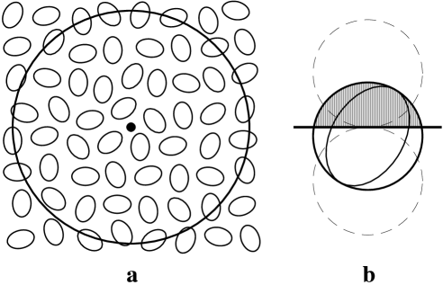
Figure 1: An electrostatic potential in a uniform isotropic medium is determined by two steps. The global one shown in panel (a) proposes the account of atomic contributions (small ovals) inside an ideal sphere (the large circle) centred at a reference point (the small filled circle) and of radius $R_{0}$ tending to infinity. Then the boundary effect associated with truncated ovals arises. In the case of an individual oval shown in panel (b) this effect includes the averaging over orientations transforming that heavy oval to a sphere (the solid circle) of radius $R$. This sphere is further truncated by the horizontal line exhibiting the boundary surface element. The charge containing in the outer part of the atomic sphere (the hatching area) is suggested to be mapped onto the surface element for neutrality. All possible truncations are restricted schematically by the dashed circles.

the spherical symmetry of $\psi(r)$, one can see that the normalized electron charge distribution necessary for (1) is equal to $\rho(r)=-(e\alpha^{3}/\pi)\exp(-2\alpha r)$, where $e$ is the elementary charge. With taking potential (1) into account, the electron contribution to the ground-state energy of the hydrogen atom with a certain electron spin projection can be written down as

$$E_{\rm mod}=\frac{\hbar^{2}\alpha^{2}}{2m_{\rm e}}-\alpha e^{2}+\frac{\pi e^{2}}{\alpha^{2}v}.$$ (2)

Here $\hbar$ is Planck’s constant, $m_{\rm e}$ is the electron mass, the last term on the right-hand side of (2) corresponds to the foregoing effect of ${\mit\Phi}_{\rm top}$, but operating on the electron part of the hydrogen atom only. This is a subtle point of the present consideration where the self-consistency of the configuration of the electron subsystem alone is studied. Moreover, a half of the effect of ${\mit\Phi}_{\rm top}$ associated with a particular spin projection seems to be plausible to be taken into account. An equilibrium value of $\alpha$ is then obtained from the condition that $E_{\rm mod}$ be a minimum. As a result, we derive

$$\frac{\hbar^{2}\alpha}{m_{\rm e}}-e^{2}-\frac{2\pi e^{2}}{\alpha^{3}v}=0$$ (3)

so that $\alpha$ becomes a function of $v$ now.

Here we are interested in the case of rarefied gas where the value of $v$ is large enough so that the value of $\alpha$ is very close to its conventional magnitude of $\alpha_{0}=m_{\rm e}e^{2}/\hbar^{2}$ in agreement with formula (3). The case of condensed matter will be discussed elsewhere. It is important that connection (3) takes place even if we come back to the general atomic energy $E$ specified by relation (2), where the last term should be omitted as applied to a neutral atom as a whole. In particular, an additional pressure effect can be expected therefrom in the form modifying an ideal gas law:

$$P=P_{\rm top}+\frac{k_{\rm B}T}{v},$$ (4)

where $k_{\rm B}$ is the Boltzmann constant, $T$ is the temperature,

$$P_{\rm top} = -\frac{\partial E}{\partial v}=-\frac{\partial E}{\partial\alpha}\frac{d\alpha}{dv}=\frac{4\pi^{2}m_{\rm e}e^{4}}{\alpha^{6}v^{3}\hbar^{2}}\Bigl{(}1+\frac{6\pi m_{\rm e}e^{2}}{\alpha^{4}v\hbar^{2}}\Bigr{)}^{-1}$$ (5)

$$\approx \frac{4\pi^{2}m_{\rm e}e^{4}}{\alpha^{6}v^{3}\hbar^{2}}.$$

The last relation corresponds to the limit of large $v$. In this case $P_{\rm top}v_{0}^{3}\approx 1.1615\cdot 10^{15}$ Pa, where the dimensionless $v_{0}$ is measured in atomic units.

It is interesting to note that both the terms on the right-hand side of equation (4) are of kinetic nature. Indeed, while the last term there is associated with the original statistical Maxwell distribution, the first one is connected with the disturbance of the kinetic intratomic energy in form (2).

The additional pressure effect obtained above immediately leads to the existence of the corresponding infrasound that is especially pronounced in the limit of zero temperature. In order to derive it, we introduce the corresponding mass density $\mu=m_{\rm p}/v$, where $m_{\rm p}$ is the proton mass. Now we cast the foregoing value of $P_{\rm top}$ in terms of $\mu$. The sound velocity of interest $c_{\rm s}$ in the limit of large $v$ is then represented as

$$c_{\rm s}^{2}=\frac{\partial P_{\rm top}}{\partial\mu}\approx\frac{12\pi^{2}}{\alpha^{6}v^{2}}\frac{m_{\rm e}e^{4}}{m_{\rm p}\hbar^{2}}=\frac{3.09\cdot 10^{11}}{v_{0}^{2}}\Bigr{(}\frac{\rm m}{\rm s}\Bigl{)}^{2}.$$ (6)

It is important that the effect mentioned above takes place only when gas in question is fixed anyhow in space. Otherwise, the value of $v$ tends to increase. In order to describe this problem we introduce Cartesian parameters of unit length $r_{x}$, $r_{y}$ and $r_{z}$, so that $r_{x}r_{y}r_{z}=v$. On the other hand, the derivatives of those length parameters with respect to time $t$ represent the corresponding velocity components $V_{\beta}=dr_{\beta}/dt$, providing that $V_{x}^{2}+V_{y}^{2}+V_{z}^{2}={\mathbf{V}}^{2}$. As a result, in the non-relativistic limit the essential part of the local energy can be written as $E_{\rm loc}=m_{\rm p}{\mathbf{V}}^{2}/2+E$, providing that every volume $v$ is specified by one atom with the proton mass $m_{\rm p}$. The conservation of this value implies that $dE_{\rm loc}/dt=0$. With taking equations (3) and (5) into account, the direct differentiation results in the following expression

$$\sum\limits_{\beta}V_{\beta}\Bigl{[}m_{\rm p}\frac{dV_{\beta}}{dt}-\frac{4\pi^{2}m_{\rm e}e^{4}}{\alpha^{6}v^{2}r_{\beta}\hbar^{2}}\Bigl{(}1+\frac{6\pi m_{\rm e}e^{2}}{\alpha^{4}v\hbar^{2}}\Bigr{)}^{-1}\Bigr{]}=0.$$ (7)

At this stage of consideration it is convenient to consider the values $V_{x}$, $V_{y}$ and $V_{z}$ as mutually independent. It implies that each of the three expressions in the square brackets in the summand of (7) be zero. On the other hand, in the isotropic case of interest we believe that all the unit-cell parameters increases in the same manner so that they can be described in the form $r_{x}=r_{y}=r_{z}=x_{0}Q$, where $Q$ is a variable dimensionless parameter. Substituting the latter relation into formula (7), where each square brackets gives the same result, we get

$$\ddot{Q}=\frac{a}{Q^{4}(Q^{3}+b)},$$ (8)

where every dot over Q stands for the derivative with respect to time, the parameters

$$a=\frac{4\pi^{2}m_{\rm e}e^{4}}{\alpha^{6}x_{0}^{8}m_{\rm p}\hbar^{2}}\qquad\mbox{and}\qquad b=\frac{6\pi m_{\rm e}e^{2}}{\alpha^{4}x_{0}^{3}\hbar^{2}}$$ (9)

are suggested to be independent of $Q$ that is right at least as $\alpha\to\alpha_{0}$. In this case equation (8) can be easily integrated and we obtain

$$\bigl{(}{\dot{Q}}\bigr{)}^{2}=\frac{2a}{3b^{2}}\Bigl{[}b\Bigl{(}1-\frac{1}{Q^{3}}\Bigr{)}+\ln\frac{Q^{3}+b}{Q^{3}(1+b)}\Bigr{]},$$ (10)

where an arbitrary constant of integration is chosen here so that ${\dot{Q}}=0$ at $Q=1$, for convenience. It implies that $Q=1$ is the initial value corresponding to a certain value of $x_{0}$ describing the state of gas before its expansion.

It is surprising that relation (10) can be addressed to the cosmological problem. Indeed, the expansion of $v$ as a local effect leading to relation (7) can happen in the most natural way on the surface of the Friedman three-dimensional hypersphere Frie22 , providing that the radius of that hypersphere increases. In this event the value ${\dot{Q}}/Q$ may be associated with the Hubble function Bart10 ; Tamm08 $H_{0}$ dependent on the initial gas density. In terms of the dimensionless parameter $h=H_{0}/(100\;{\rm km}\;{\rm s}^{-1}{\rm Mpc}^{-1})$ the results are shown in Fig. 2. According to (10), it implies that the expansion predicted here is not

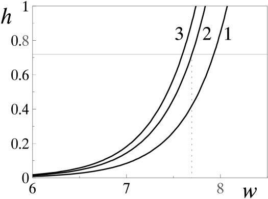
Figure 2: The dimensionless Hubble parameter $h$ in dependence on the initial gas density $n_{\rm ini}$ in units of $10^{w}$ atoms/m³. Curves 1, 2 and 3 correspond to the final gas density equal to 1, 5 and 10 atoms/m³, respectively. The thin horizontal line describes the present value of the Hubble constant adopted as $h=0.719$. For curve 2 it corresponds to $n_{\rm ini}\approx 5\cdot 10^{7}$ atoms/m³, as shown by the vertical dotted line.

associated with the Big Bang. The initial gas density may thus be regarded as the threshold one above which any fluctuation of distinct nature can be expected.

The time of expansion up to a given $Q$ can in turn be obtained upon further appropriate integration of equation (10):

$$t=b\sqrt{\frac{3}{2a}}\int\limits_{1}^{Q}\Bigl{[}b\Bigl{(}1-\frac{1}{u^{3}}\Bigr{)}+\ln\frac{u^{3}+b}{u^{3}(1+b)}\Bigr{]}^{-1/2}du.$$ (11)

Relation (11) is simplified in the particular limit of small gas concentrations. In this case we obtain the conventional relation Bart10 $t\approx H_{0}^{-1}$. In the particular event singled out in Fig. 2 the time of interest becomes equal to 13.6 Gyr in agreement with the evaluations known in the literature Peeb03 ; Bart10 .

Here we consider the self-consistent effect of the topological field of the Coulomb nature in its simplest form with only one configuration parameter $\alpha$. In general, the same effect still exists, but the consideration is expected to be more complicated.

P.S. This paper was submitted to Nature (2012-05-06944), Nature Physics (NPHYS-2012-06-01221-T), Nature Chemistry (NCHEM-12060801-T) and Nature Materials (NM12061695-T).

References

- (1) Tosi, M. P. in Solid State Physics Vol. 16 (eds Seitz, F. & Turnbull, D.) 1–120 (Academic Press, 1964).
- (2) Harris, F. E. in Theoretical Chemistry: Advances and Perspectives Vol. 1(eds Eyring, H. & Henderson, D.) 147–218 (Academic Press, 1975).
- (3) Ewald, P. P. Die Berechnung optischer und elektrostatischer Gitterpotentiale. Ann. Phys. 64, 253–287 (1921).
- (4) Born, M. & Huang, K. Dynamical Theory of Crystal Lattices (Clarendon Press, 1954).
- (5) Kholopov, E. V. Convergence problems of Coulomb and multipole sums in crystals. Usp. Fiz. Nauk 174, 1033–1060 (2004) [Phys. — Usp. 47, 965–990 (2004)].
- (6) Kholopov, E. V. A simple general proof of the Krazer-Prym theorem and related famous formulae resolving convergence properties of Coulomb series in crystals. J. Phys. A: Math. Theor. 40, 6101–6117 (2007).
- (7) Kholopov, E. V. Multiple charge spreading as a generalization of the Bertaut approach to lattice summation of Coulomb series in crystals. Physica B: Condens. Matter 405, 2883–2890 (2010).
- (8) Kholopov, E. V. in New Topics in Mathematical Physics Research (ed Benton, C. V.) 241–303 (Nova Science Publishers, 2006).
- (9) Kholopov, E. V. Mean potential of Bethe in the classical problem of calculating bulk electrostatic potentials in crystals. Phys. Stat. Sol. B 243, 1165–1181 (2006).
- (10) Friedman, A. Über die Krümmung des Raumes. Z. Phys. 10, 377–386 (1922).
- (11) Riess, A. G., Filippenko, A. V., Challis, P., Clocchiatti, A., Diercks, A., Garnavich, P. M., Gilliland, R. L., Hogan, C. J., Jha, S., Kirshner, R. P., Leibundgut, B., Phillips, M. M., Reiss, D., Schmidt, B. P., Schommer, R. A., Smith, R. C., Spyromilio, J., Stubbs, C., Suntzeff, N. B. & Tonry, J. Observational evidence from supernovae for an accelerating Universe and a cosmological constant. Astron. J. 116, 1009–1038 (1998).
- (12) Schmidt, B. P., Suntzeff, N. B., Phillips, M. M., Schommer, R. A., Clocchiatti, A., Kirshner, R. P., Garnavich, P., Challis, P., Leibundgut, B., Spyromilio, J., Riess, A. G., Filippenko, A. V., Hamuy, M., Smith, R. C., Hogan, C., Stubbs, C., Diercks, A., Reiss, D., Gilliland, R., Tonry, J., Maza, J., Dressler, A., Walsh, J. & Ciardullo, R. The high- supernova search: Measuring cosmic deceleration and global curvature of the Universe using type Ia supernovae. Astrophys. J. 507, 46–63 (1998).
- (13) Perlmutter, S., Aldering, G., Goldhaber, G., Knop, R. A., Nugent, P., Castro, P. G., Deustua, S., Fabbro, S., Goobar, A., Groom, D. E., Hook, I. M., Kim, A. G., Kim, M. Y., Lee, J. C., Nunes, N. J., Pain, R., Pennypacker, C. R., Quimby, R., Lidman, C., Ellis, R. S., Irwin, M., McMahon, R. G., Ruiz-Lapuente, P., Walton, N., Schaefer, B., Boyle, B. J., Filippenko, A. V., Matheson, T., Fruchter, A. S., Panagia, N., Newberg, H. J. M. & Couch, W. J. Measurements of and from 42 high-redshift supernovae. Astrophys. J. 517, 565–586 (1999).
- (14) Peebles, P. J. E. & Ratra, B. The cosmological constant and dark energy. Rev. Mod. Phys. 75, 559–606 (2003).
- (15) Chernin, A. D. Dark energy and universal antigravitation. Usp. Fiz. Nauk 178, 267–300 (2008) [Phys. — Usp. 51, 253–282 (2008)].
- (16) Lukash, V. N. & Rubakov, V. A. Dark energy: myths and reality. Usp. Fiz. Nauk 178, 301–308 (2008) [Phys. — Usp. 51, 283–290 (2008)].
- (17) Bartelmann, M. The dark Universe. Rev. Mod. Phys. 82, 331–382 (2010).
- (18) Tammann, G. A., Sandage, A. & Reindl, B. The expansion field: The value of . Astron. Astrophys. Rev. 15, 289–331 (2008).