Structure and Controls of the Global Virtual Water Trade Network

Abstract

Recurrent or ephemeral water shortages are a crucial global challenge, in particular because of their impacts on food production. The global character of this challenge is reflected in the trade among nations of virtual water, i.e. the amount of water used to produce a given commodity. We build, analyze and model the network describing the transfer of virtual water between world nations for staple food products. We find that all the key features of the network are well described by a model that reproduces both the topological and weighted properties of the global virtual water trade network, by assuming as sole controls each country’s gross domestic product and yearly rainfall on agricultural areas. We capture and quantitatively describe the high degree of globalization of water trade and show that a small group of nations play a key role in the connectivity of the network and in the global redistribution of virtual water. Finally, we illustrate examples of prediction of the structure of the network under future political, economic and climatic scenarios, suggesting that the crucial importance of the countries that trade large volumes of water will be strengthened.

Gindraft=false Suweis et al. Structure and Controls of the GVWTN

1 Introduction

Food production is by far the most freshwater-consuming process (80% of the total world water resources (Rost et al., 2008)). Due to population growth and economic development, water shortage is thus subject to increasing pressure at local and global scales. Several studies have recently focused on the issues of globalization of water (e.g. Hoekstra, 2002; Chapagain et al., 2006; D’Odorico et al., 2010), using the concept of virtual water (VW) (Allan, 1993). They have highlighted the importance of tackling water management problems not only at the basin or country scales, but rather through a worldwide perspective (Hoekstra and Chapagain, 2008). Nevertheless a complete statistical characterization describing the network of VW transfers on a global scale has only started (Konar et al., 2011) and a model to explain such characteristics is still lacking.

This Letter deals with a novel theoretical network model that robustly describes topological and weighted properties of the global VW trade network (GVWTN) for the characterization of the VW flows of $5$ major crops (barley, corn, rice, soy, and wheat) and $3$ livestock products (beef, poultry, and pork). The VW content of such commodities are calculated for each nation using a state-of-the-art global water resources model (Hanasaki et al., 2008, 2010), at a spatial scale of $0.5^{o}\times 0.5^{o}$. Combining the model outputs with the data of the international trade of food products referred to the year 2000 (FAO, 2000a), the VW flows among nations are obtained (see Konar et al. (2011) and Auxiliary Materials for details) and compared with model results. Of particular interest is deemed our predictive use of the model to analyze the impact of future scenarios of social, economic, and climate change.

2 Structure of the GVWTN

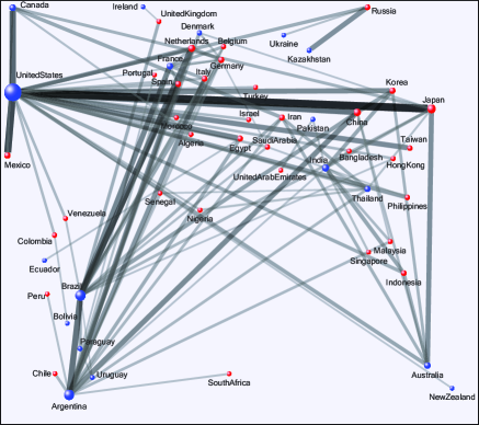
Figure 1: Backbone of the global Virtual Water Trade Network (GVWTN). Only 4% of the total number of links accounting for 80% of the total flow volume are shown. Resulting isolated nodes are consequently removed. The blue nodes represent the net exporter nations, while the red ones are the net importers. The weights of the links are color-coded by the grayscaling in the edge’s colors (black is the link carrying the highest volume of VW.)

Here we briefly present and interpret key statistical characterizations of the GVWTN (addressed in Konar et al. (2011)). For simplicity we discuss here the undirected network case, where $W$ is a symmetric matrix whose elements ($w_{ij}=w_{ji}$) represent the total volume of VW exchanged between countries (nodes) and obtained by summing the corresponding import and export fluxes (Figure 1). For mathematical details and analysis of the directed network see Auxiliary Materials.

The global topology of a network is described by its degree probability density function (pdf) $p(k)$, i.e. $p(k)dk$ is the probability that the degree of a given node is $k$ (Newman et al., 2006) (Figure 2a). It provides the number of edges connected to a given node regardless of the identity of the neighbors. To investigate how nodes are connected, we study the average nearest neighbor degree $k_{nn}$ which shows a tendency of the nodes with high degree to provide connectivity to small degree nodes (Figure 2c). Such trend (known as disassortative behavior) denotes, differently from purely random networks, non-trivial nodal degree correlations (Newman, 2002). Another interesting indicator is the local clustering coefficient $C_{i}$ ($0\leq C_{i}\leq 1$) which describes the ability of node $i$ to form cliques, i.e. triangles of connected nodes. Figure 2d shows that poorly connected nations $i$ tends to form connected trading food sub-markets ($C_{i}\approx 1$). On the contrary, high degree vertices $j$ connect otherwise disconnected regions ($C_{j}\ll 1$). The average clustering coefficient is very high ($\bar{C}=0.747$) and the graph has, in analogy to many real networks (Newman et al., 2006), an average node-to-node topological distance ($d_{nn}$) smaller than 5 ($d_{nn}=4$) (Konar et al., 2011). The GVWTN thus exhibits a small-world network behavior (Watts and Strogatz, 1998), providing a quantitative measure of the globalization of water resources (Hoekstra and Chapagain, 2008; D’Odorico et al., 2010).

The hydrological features of the network are given by its weighted properties. The total volume imported and exported by nation $i$ is quantified by its strength $s_{i}$, defined as the total VW volume exchanged by node $i$. The strength distribution shows a heavy-tailed pdf suggesting high heterogeneity of the volumes of traded VW (Figure 2b): only 4% of the total number of links accounts for 80% of the total flow volume (Konar et al., 2011), indicating established bonds among countries that rule the main fluxes in the GVWTN (Figure 1). Strengths between neighboring nodes are correlated. In fact, the average nearest neighbor strength $s_{nn}$ (Serrano, 2008) displays a decreasing trend as a function of $s$ (Figure 2e). Strength-strength correlations disentangled from degrees ($s^{W}_{nn}$) (Serrano, 2008) are not significant, i.e. $s^{W}_{nn}$ does not depend on $s$. A power-law relation $s\sim k^{b}$ with exponent $b=2.60$ (Konar et al., 2011) indicates a non-trivial correlation between node degrees and strengths (Barrat et al., 2004). The above suggests that we live in a global water world where, on average, the export of VW from few water rich countries increases the food locally available to the connected nations. At the same time, there exist preferential VW routes, mainly driven by geographical, political and economical factors, through which most of the VW volume flows.

3 Controls of the GVWTN

The complexity of all factors (political, economical and environmental) involved in shaping the GVWTN structure is remarkable, and calls for investigating whether key variables and linkages exist through which the emerging structural properties of the network could be revealed. We have developed a model that allows us to describe concisely all the above features of the GVWTN. Specifically, we assume that the topological and weighted features of the network can be determined, respectively, by two external characteristics of each node: namely, the gross domestic product (World Bank, 2010) ($GDP$) and the (average) yearly rainfall [mm/yr] on agricultural area [km²] (denoted by $RAA$ [mm$\cdot$km²/yr]).

Toward this end, each of the 184 nodes is assigned a normalized value of the $GDP$ ($x$) and $RAA$ ($y$) based on data from 2000 (United Nations, 2010; World Bank, 2010) (i.e., $x_{i}=GDP_{i}/\sum_{j=1}^{N}GDP_{j}$, $y_{i}=RAA_{i}/\sum_{j=1}^{N}RAA_{j})$. We refer to these variables as fitness (or hidden) variables (e.g. Bianconi and Barabasi, 2001; Caldarelli et al., 2002; Boguna and Pastor-Satorras, 2003; Garlaschelli and Loffredo, 2004; Park and Newman, 2004). They measure the relative importance of the vertices in the GVWTN. $GDP$ and $RAA$ are assumed to be good candidates to explain the structure of the GVWTN. In fact the country $GDP$ is closely related to its trade activity (Garlaschelli and Loffredo, 2004), while volumes of VW traded depend on the amount of crops and meat produced in that country, that in turn depends on the $RAA$. A good agreement between data and model results proves these facts. The fitness network-building algorithm consists of the following steps: $a)$ we connect every couple of vertices, $i$, $j$, (with $i\neq j$) with a probability $p(x_{i},x_{j})=\sigma x_{i}x_{j}/(1+\sigma x_{i}x_{j})$; $b)$ we assign to each link between $i$ and $j$ a weight $\langle w_{ij}\rangle$ with value given by $q(y_{i},y_{j})=\eta y_{i}y_{j}$. The parameters of the model are $\sigma$ and $\eta$ and they are determined by the compatibility conditions: $\frac{1}{2}\sum_{i}\sum_{j\neq i}p(x_{i};x_{j})=L$ and $\frac{1}{2}\sum_{i}\sum_{j\neq i}q(y_{i},y_{j})=\Phi$, where $L$ is the total number of edges in the network and $\Phi$ the total flux. No tuning of the parameters is carried out and all results presented here correspond to the above choice for $\sigma$ and $\eta$. For details on the model and its generalization to the directed network case see Appendix and Auxiliary Materials.

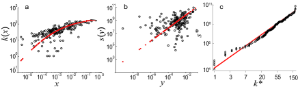
Figure 3: Comparison between empirical (black dots) and model results (red dots): a) The relationship between nodal degrees $k$ and normalized $GDP$ $x$ shows how on average the number of connections is an increasing function of the nation’s $GDP$; b) The relationship between node strength $s$ and normalized $RAA$, $y$ i.e. $s(y)=N\eta\langle y\rangle y$; c) The node independent relationship between strengths $s^{*}$ and degrees $k^{*}$ in the GVWTN ($s^{*}\sim{k^{*}}^{q}$). The red line represents the best fit obtained from $k$ and $s$ generated by the fitness model. In this case, we find $q=2.69\pm 0.03$ ($R^{2}=0.98$). All the plots are in log-log scale.

The model predicts that for each country the number of food trade partners grows non linearly with its $GDP$ (similarly to the world trade web (Garlaschelli and Loffredo, 2004)), while the total exported and imported VW is found proportional to the $RAA$. Exact results are obtained on the properties related to the node strengths (see Appendix for details). The analytical results match closely the empirical ones. In particular we find that $\langle s(y)\rangle=N\eta\langle y\rangle y$ (where $\langle\cdot\rangle$ represents the ensemble average and $s(y)$ is the strength of a node associated with the value $y$ of the normalized $RAA$), $\langle s^{W}_{nn}\rangle=N\eta\gamma^{2}\Gamma[1+2/\beta]$ (where $\Gamma[\cdot]$ is the complete Gamma function) and that the pdf of the node strength is $p(s)=\mathcal{C}s^{\beta-1}e^{(-\frac{s}{\gamma\eta})^{\beta}}$, where $\mathcal{C}=\beta/(\gamma\eta)^{\beta}$ with $\beta\approx 0.482$ and $\gamma\approx 0.002$ parameters related to the pdf of $y$ (see Auxiliary Materials for details). From the empirical relation $s=ak^{b}$ it can be shown that the cumulative degree pdf decays exponentially as $P_{>}(k)=\int_{k}^{\infty}p(k^{\prime})dk^{\prime}=e^{-\alpha k^{\beta b}}$, with $\alpha=(\gamma\sigma/a)^{-\beta}$ and $\beta\cdot b\approx 1.25$. Figures 2 and 3 summarize all the results discussed above. They show the excellent agreement of the fitness model with the empirical data.

4 Future Scenarios

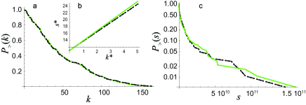
Figure 4: An example of predictive application of the fitness model of GVWTN for the driest case scenario: comparison between the global properties of the network for the year 2000 (dashed black) with those predicted by the fitness model for the year 2030 (green line): a) Cumulative degree pdf. Inset b): Relationships between sorted strengths and degrees); c) Cumulative pdf of the nodal strengths.

Our theoretical framework is suitable to investigate future scenarios of the GVWTN structure. To this aim, we evaluate estimates of the annual rainfall for 2030-2050 from the A2 socio-economic scenario of the World Climate Research Programmes (WCRPs) Coupled Model Intercomparison Project Phase 3 (CMIP3) multi-model dataset (Meehl et al., 2007). The spatial mean is then calculated for each country in the network over this time horizon. Then by using published projections of the $GDP$ and agricultural area (FAO, 2000b; Fonseca et al., 2009) for 2030, we build the fitness functions $p(x^{T}_{i},x^{T}_{j})=\sigma^{\prime}x^{T}_{i}x^{T}_{j}/(1+\sigma^{\prime}x^{T}_{i}x^{T}_{j})$ and $q(y^{T}_{i},y^{T}_{j})=\eta^{\prime}y^{T}_{i}y^{T}_{j}$, where $x^{T}$ and $y^{T}$ are the projections of the fitness variables at year $T=2030$. The parameters $\sigma^{\prime}$ and $\eta^{\prime}$ are to be determined by the future total number of connections $L^{\prime}$ and flux $\Phi^{\prime}$. In our simulation we assumed that $L^{\prime}=L$ and $\Phi^{\prime}=\Phi$, but in general they may be part of the scenarios under study. All A2 climate change scenarios (Meehl et al., 2007) yield a decrease in rainfall at a global scale, but the total arable land is predicted by (FAO, 2000b) to increase around 1%, thereby leading to an increase of the total $RAA$. Figure 4 summarizes the results of the structure of the GVWTN under the driest climate change scenario. We find that the structure of the GVWTN topology is robust with respect to these particular scenarios. A heavier tail in the strengths pdf is observed suggesting a rich-gets-richer phenomenon (Newman et al., 2006), where the nodes with large strengths benefit from the changes in $RAA$, becoming even stronger. We also find that the exponent in the node independent relation $s^{*}\sim{k^{*}}^{q}$, (where the vectors $k^{*}$ and $s^{*}$ are the sorted degrees and strengths in the GVWTN) increases from $q=2.69\pm 0.03$ ($R^{2}=0.982$) to $q=2.77\pm 0.02$ ($R^{2}=0.986$) (see Figure 3c and inset Figure 4b). These results suggest that economic and climatic future scenarios will likely enhance the globalization of water resources, giving to water-rich countries even more inroad for reaching poorly connected nodes. At the same time, the observed rich-gets-richer phenomenon will intensify the reliance of most of the nations on the few VW hubs. As a consequence it will reduce the ability of the GVWTN to respond to disturbances whose impact may be dramatic when the VW trade supports carrying capacities beyond those supported by local resources (D’Odorico et al., 2010). Finally our study highlights how agricultural land management may indeed remarkably impact the future structure of the GVWTN.

Our work opens new quantitative and predictive perspectives in the study of stability and complexity of the GVWTN coupled to social, economic and political processes related to the international food trade. Ongoing research incorporates scenarios where $L^{\prime}$ and $\Phi^{\prime}$ are different from values of the year 2000 and reflect the evolving and dynamic character of the global network.

Appendix

Our modelling scheme for the properties of the GVWTN employs: i) a function describing the topological properties of the network, and ii) a function, independent of i), characterizing its weights. The functional shape of $p(x_{i},x_{j})$, the probability that node $i$ and $j$ – endowed respectively with fitness $x_{i}$ and $x_{j}$ – are connected, is found through an entropy optimization principle and by imposing that all graphs with degree sequence $\{k_{l}\}_{l=1,2,..}$ appear in our ensemble with equal probability (see Auxiliary Materials and Park and Newman (2004) for details). The result is

$$p(x_{i},x_{j})=\frac{\sigma x_{i}x_{j}}{1+\sigma x_{i}x_{j}}.$$ (1)

The key assumption is that fitness variable $x_{i}$ is assumed to be the external quantity $x_{i}=GDP_{i}/(\sum_{j}GDP_{j})$, determining the topological importance of node $i$ by driving the number of its connections. From Eq. (1) one computes all topological properties (defined in the Auxiliary Materials): the node degree $\langle k_{i}\rangle=\sum_{j\neq i}^{N}p(x_{i},x_{j})$; the average degree of the nearest neighbors

$$\langle k_{nn,i}\rangle=\frac{\sum_{j\neq i}^{N}\sum_{l\neq j}p(x_{i},x_{j})p(x_{j},x_{l})}{\langle k_{i}\rangle},$$ (2)

and the local clustering coefficient:

$$\langle C_{i}\rangle=\frac{\sum_{j\neq i}^{N}\sum_{l\neq j,i}^{N}\ p(x_{i},x_{j})p(x_{j},x_{l})p(x_{l},x_{i})}{(\langle k_{i}\rangle-1)\langle k_{i}\rangle}.$$ (3)

A function $q(y_{i},y_{j})$ assigns the average weight $\langle w_{ij}\rangle$ to the link connecting $i$ to $j$ as a function of the fitness variables $y$. We interpret $\langle w_{ij}\rangle$ as a rank associated with the assigned link between two nodes $i$ and $j$ and its importance. By generalizing the concept of weighted configuration model (Serrano and Boguna, 2005; Garlaschelli and Loffredo, 2009), our null hypothesis for $q(y_{i},y_{j})$ is:

$$q(y_{i},y_{j})=\eta y_{i}y_{j},$$ (4)

where $\eta$ is the parameter controlling the total flux of the network. We choose as fitness variable $y$ the normalized rainfall on agricultural area $y_{i}=RAA_{i}/\sum RAA_{i}$.

Given the simple functional shape of Eq. (4), if an analytical approximation for the distribution of $y$ exists, exact results can be obtained on the properties involving node strengths. We find that the empirical cumulative distribution of $y$ is well fitted ($R^{2}\approx 0.998$) by a stretched exponential $\rho_{>}(y)=\exp\left(-(\frac{y}{\gamma})^{\beta}\right)$. Then using the continuum approximation (Caldarelli et al., 2002), we obtain $\langle s(y)\rangle=N\int_{0}^{\infty}q(y,z)\rho(z)dz=N\langle y\rangle\eta y=NF(y)$, and for large enough $N$ one has: $p(s)=\rho[NF^{-1}(s/N)]\frac{d}{ds}F^{-1}(s/N)=\frac{1}{\eta}\rho(s/\eta)$, yielding:

$$P_{>}(s)=e^{-(\frac{s}{\eta\gamma})^{\beta}}.$$ (5)

Finally, the strength-strength correlation ia obtained as:

$$\langle s^{W}_{nn}(y)\rangle=\frac{N\int_{0}^{\infty}q(y,z)\langle s(z)\rangle\rho(z)dz}{\langle s(y)\rangle}=N\eta\gamma^{2}\Gamma[1+2/\beta],$$ (6)

and it is found that it that does not depend on $y$. Although we are not able to repeat the same procedure for the fitness variable $x$, a qualitative analytical behavior for the distribution of the node degree can be obtained by using the empirical relation $s=ak^{b}$ through a derived distribution approach, i.e. $p(k)dk=p(s)ds$. We then find:

$$P_{>}(k)=e^{-(\frac{a}{\eta\gamma})^{\beta}k^{b\beta}},$$ (7)

which is a compressed exponential distribution, confirming the exponential-like tail observed from the empirical analysis of the degree distribution. Further details are in the Auxiliary Materials.

Figure 2: Topological and weighted properties of the GVWTN compared with the results of the fitness model (red line). a-b) Cumulative pdf of the node’s degree $P_{>}(k)$ in linear scale and node strength $P_{>}(s)$ in log-log scale; c-d) average nearest neighbors degree $k_{nn}$ and cluster coefficient $C$ as a function of the nodes degree $k$; e-f) average nearest neighbors strength $s_{nn}$ and strengths-strengths correlation $s^{W}_{nn}(s)\sim const$ in semilog-$x$ and log-log scale, respectively.