Non-linear density-velocity divergence relation from phase space dynamics.
Abstract
We obtain the non-linear relation between cosmological density and velocity perturbations by examining their joint dynamics in a two dimensional density-velocity divergence phase space. We restrict to spatially flat cosmologies consisting of pressureless matter and non-clustering dark energy characterised by a constant equation of state . Using the spherical top-hat model, we derive the coupled equations that govern the joint evolution of density and velocity perturbations and examine the flow generated by this system. In general, the initial density and velocity are independent, but requiring that the perturbations vanish at the big bang time sets a relation between the two. This traces out a curve in the instantaneous phase space, which we call the ‘Zel’dovich curve’. We show that this curve acts like an attracting solution for the phase space dynamics and is the desired non-linear extension of the density-velocity divergence relation. We obtain a fitting formula which is a combination of the formulae by Bernardeau and Bilicki & Chodorowski, generalised to include the dependence on . We find that as in the linear regime, the explicit dependence on the dark energy equation of state stays weak even in the non-linear regime.Although the result itself is somewhat expected, the new feature of this work is the interpretation of the relation in the phase space picture and the generality of the method. Finally, as an observational implication, we examine the evolution of galaxy cluster profiles using the spherical infall model for different values of . We demonstrate that using only the density or the velocity information to constrain is subject to degeneracies in other parameters such as but plotting observations onto the joint density-velocity phase space can help lift this degeneracy.
keywords:
cosmology: theory - cosmology: dark energy - cosmology: large-scale structure of Universe - galaxies: clusters: general1 Introduction
The distribution of matter on very large scales ( Mpc) is fairly homogenous (e.g., Hogg et al. 2005, Sarkar et al. 2009, Scrimgeour et al. 2012), but on smaller scales it is far from it. The fractional overdensity () and the peculiar velocity () are the two variables that characterise this inhomogeneity and are related via the continuity equation, the Euler equation and the law of gravitation. When the inhomogeneities are small, the equations can be linearised and ignoring the decaying mode results in the local relation , where is the Hubble parameter and is the linear growth factor. In the theory of gravitational instability, except in the orbit-crossing regions, the peculiar velocity is curl free and the above equation completely characterises the relation between the two fields in the linear regime. mainly depends on the matter density parameter , and is usually expressed as , where is the growth index. Given , a comparison of the data from redshift and peculiar velocity surveys constrains , or some combination of and the galaxy bias parameter. Early studies in this field mostly assumed a pure matter universe and used (Peebles 1976), to either get bias independent measures of mass from velocity fields or to constrain (see review articles by Dekel 1994 and Strauss & Willick 1995). The estimate by Peebles, given more than thirty five years ago, turned out to be a good approximation for a large range of models. The dependence of the linear growth rate on the cosmological constant (for e.g., Martel 1991; Lahav et al. 1991) or on the dark energy equation of state (Wang & Steinhardt 1998; Linder 2005) was shown to be relatively weak. However, more recently, it has been pointed out that models with similar expansion histories but with different gravitational dynamics can be distinguished by their growth indices; is 0.55 for the CDM model, but 0.67 for certain modified theories of gravity (Lue, Scoccimarro, & Starkman 2004; Bueno Belloso, García-Bellido, & Sapone 2011). Accordingly, modern observational efforts are focussed on measuring the linear growth rate with the added aim of constraining (for e.g., Guzzo et al. 2008; Majerotto et al. 2012).
The method of velocity reconstruction from redshift surveys using linear theory breaks down when the perturbations are of order unity. Quasi-linear effects need to be included even to get an accurate determination of the linear growth rate (Nusser, Branchini, & Davis 2012). Various analytic quasi-linear and non-linear extensions using the Zel’dovich approximation (Nusser et al. 1991; Gramann 1993a), second order Eulerian perturbation theory (Bernardeau 1992, hereafter B92), and higher order Lagrangian perturbation theory (Gramann 1993b; Chodorowski & Łokas 1997; Chodorowski et al. 1998; Kitaura et al. 2012) have been proposed. Many of these analytic methods were also tested with numerical simulations (Mancinelli et al. 1993; Mancinelli & Yahil 1995). N-body codes, although accurate, give mass-weighted instead of volume-weighted estimates (Dekel, Bertschinger, & Faber 1990) making it difficult to compare them with analytical answers. Refined volume averaged estimates were given using uniform-grid codes (Kudlicki et al. 2000; Cieciela̧g et al. 2003) and the method of tessellations (Bernardeau & van de Weygaert 1996; Bernardeau et al. 1997, Bernardeau et al. 1999). In general, these simulations are slow and are applicable to a limited range of models. It is usually assumed that the weak dark energy dependence of the linear relation extends to the non-linear regime and often the results are quoted in terms of the scaled velocity divergence , absorbing the cosmology dependence into the linear growth rate. While this assumption has been tested for different values of the cosmological constant (for e.g., Lahav et al. 1991; Bouchet et al. 1995; Nusser & Colberg 1998), the explicit dependence on the dark energy equation of state has not yet been derived.
The spherical top-hat system is an alternate way to model evolution in the non-linear regime. The model is simple to solve; equations of motion reduce to ordinary second order differential equations for the evolution of the scale factor (Peebles 1980). The main drawback is that it does not take into account interaction between scales; the price paid for computational ease. Nevertheless, it has been successful in predicting non-linear growth until virialization (Engineer et al. 2000; Shaw & Mota 2008). Recently Bilicki & Chodorowski (2008), hereafter BC08, obtained the non-linear density-velocity relation from the spherical top-hat. They utilised the top-hat’s known exact analytic solutions and hence were restricted to pure matter cosmologies. We adopt a different approach, one that can be generalised to a range of background cosmologies. We numerically investigate how generic density and velocity perturbations evolve in a two dimensional density-velocity divergence phase space. We identify a special curve which is obtained by imposing the condition that the perturbations vanish at the big bang time and show that it acts like an attracting solution for the dynamics of the system. We refer to this as the ‘Zel’dovich curve’ and demonstrate that it is the desired density-velocity relation in the non-linear regime. This approach was first put forward in a recent paper (Nadkarni-Ghosh & Chernoff 2011, hereafter NC), but the analysis there was restricted to a EdS (with ) cosmology. Here we extend the same idea to flat cosmological models with pressureless matter and non-clustering dark energy described by a constant equation of state .
The paper is organised as follows. §2 gives the equations governing the spherical top hat, introduces the ‘Zel’dovich curve’ and demonstrates its importance in the evolution of perturbations in the joint density-velocity phase space. §3 gives a fit to the curve by generalising the formulae proposed by B92 and BC08 to include the dark energy term and this results in a new parametrization for the linear growth index as a function of . §4 discusses the evolution of galaxy cluster profiles using the spherical infall model and examines this curve in the context of observationally relevant quantities. §5 gives the summary and conclusion.
2 Dynamics of the spherical top-hat
2.1 Physical set-up and equations
The compensated spherical top-hat perturbation consists of a uniform density sphere surrounded by a concentric spherical compensating region; homogenous and isotropic background extends beyond the outer edge of this region. The compensating shell could be empty or contain mass depending upon whether the inner sphere is overdense or underdense with respect to the background. In this paper we restrict ourselves to flat background cosmologies comprising of pressureless matter and dark energy. Only matter perturbations are considered. The total matter density and Hubble parameter are denoted as and for the background (perturbation). Dark energy is assumed to be spatially uniform and does not interact with the matter fields. It is described by a constant (in time) equation of state parameter defined as , where and are the dark energy pressure and density respectively.
The evolution of the background is completely determined by specifying , and at some initial time . The governing equation is
| (1) |
where the dots represent derivatives with respect to time and are the initial matter (dark energy) density parameters. The initial conditions for eq. (1) are and .
The perturbation at the initial time is described by two quantities: the fractional overdensity and the fractional Hubble parameter defined as
| (2) | |||||
| (3) |
In the case of a pure matter cosmology, Birkoff’s theorem guarantees that the inner sphere can be described as a separate independent universe, whose scale factor obeys an equation analogous to eq. (1), but with a different value for the matter density parameter. In the presence of a dark energy term the modification is not always obvious as has been discussed by various authors (Pace, Waizmann, & Bartelmann 2010; Wintergerst & Pettorino 2010). We follow the approach advocated in these papers of starting with the exact non-linear hydrodynamic equations for the density and velocity instead of an equation for the perturbation scale factor (for e.g., Lima, Zanchin, & Brandenberger 1997; Abramo et al. 2007). By recasting the Eulerian system in Lagrangian coordinates, one can show that for scales much smaller than the horizon scale and in the absence of matter-dark energy interactions, the spherical top-hat can be described by a scale factor which obeys
| (4) |
with initial conditions and (see Appendix A for details). In cosmology, the initial time is usually the time of recombination, after which perturbations start to grow. However, we will allow it to be specified anywhere between the big bang time (when ) and today (when ). , , , and refer to the initial values at the specified initial epoch .
The Hubble parameter and the density parameters () at any arbitrary epoch are related to those today (, ) through
| (5) | |||||
| (6) | |||||
| (7) |
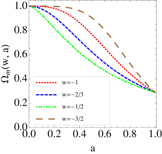
The last two equalities follow from the definition of , the relation between and the critical density and the scalings , . The evolution of is plotted in figure 1 for four different values of the equation of state . Flatness implies at all epochs. and are fixed to be 0.29 and 0.71 in accordance with recent results from Type IA supernovae (SN Ia) and Wilkinson Microwave Anisotropy Probe (WMAP) data (Kowalski et al. 2008, Komatsu et al. 2011). From these results is known to be close to ; we choose four values . All models are matter dominated at early epochs () and have the same matter density at late epochs. But at intermediate epochs, is different for the four models. Dark energy dominates earlier for larger values of . For the EdS cosmology, and for all epochs.
Once the solutions to eqs. (1) and (4) are known, the perturbation parameters at any later time can be computed
| (8) | |||||
| (9) |
The perturbation variable is related to the usual peculiar velocity divergence as
| (10) |
In the rest of the paper we refer to as simply ‘density’ and peculiar velocity as simply ‘velocity’.
The spherical top-hat serves as a proxy for the non-linear regime only to the extent that it models density contrasts much higher than unity. It does not model non-linearities in truly inhomogeneous systems where different scales in the system interact to give non-local effects. In such cases the relation has a scatter and can no longer be described by a one-to-one function. The ‘forward’ relation (mean density in terms of the velocity divergence) and the ‘inverse’ relation (mean velocity divergence in terms of the density) are not mathematical inverses of each other and it is more informative to describe the relation by a joint probability distribution function for the two variables (Bernardeau et al. 1999). These relations have been obtained for CDM and CDM cosmologies using perturbation theory (e.g., B92; Chodorowski & Łokas 1997; Chodorowski et al. 1998) as well as simulations (e.g., Bernardeau et al. 1999; Kudlicki et al. 2000). The relation obtained from the top-hat is local and is expected to be applicable only in a average sense.
2.2 The Zel’dovich curve
Consider the two-dimensional phase space whose abscissa and ordinate are and respectively. Mathematically, the initial value of and are independent choices and this freedom allows for solutions where the perturbation scale factor is non-zero at the big bang time. However, physically, it is reasonable to expect that there were no perturbations at the big bang epoch i.e., the scale factors of the background and the perturbation are both zero at the big bang and start evolving since then. This condition sets a specific relationship between the initial and . If we define the age at time to be the time taken for the scale factor to grow from zero to its value at then this condition is equivalent to demanding that the ages of the background and perturbation be the same. For any starting epoch, this relation traces out a curve in the phase space. The ‘equal age’ condition is imposed in linear theory by ignoring the decaying modes in the solution for . This assumption also forms the basis of the Zel’dovich approximation (Zel’Dovich 1970) and hence we refer to this special curve as the ‘Zel’dovich curve’.
In NC this curve was examined for the EdS cosmology. In this special case, from eqs. (1) and (4), one can explicitly calculate the ages of the background and perturbation and the ‘equal age’ condition becomes (see Appendix B)
| (11) |
This relation does not involve any time dependent quantities and the Zel’dovich curve has the same form at all epochs. However, in the presence of generic dark energy terms, this relation has a time dependence. This can be seen by scaling and in eqs. (1) and (4) by and replacing time by . The equations and initial conditions depend only on the parameters and (flatness removes dependence). The ‘equal age’ criterion remains unchanged by this scaling and the resulting relation depends only on the parameters and . Since the value of changes with the starting epoch, the relation will be different at different epochs. For the kind of dark energy models considered here, analytic solutions for eqs. (1) and (4) are somewhat tedious, if at all possible (Lee & Ng 2010), and we solve the equations numerically. Appendix B gives the details of the calculation.
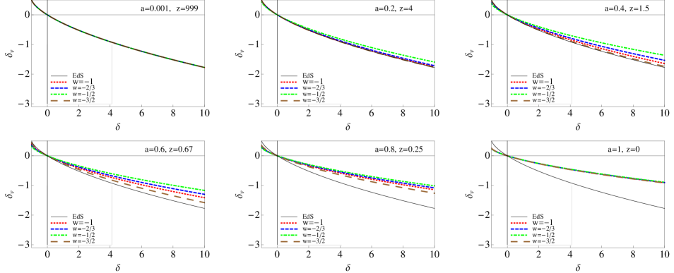
Figure 2 shows the Zel’dovich curves for different cosmological models. Brown (long dashed), red (dotted), blue (short dashed) and green (dot dashed) lines correspond to and respectively. The black curve, given by eq. (11), corresponds to the EdS model. Six different epochs between and or, equivalently, between and are considered. At recombination (), the curves for different overlap with each other and with the EdS case. At they again overlap, but differ from the EdS case. At intermediate epochs, they differ from each other. Comparison with figure 1 suggests that the Zel’dovich curve mainly depends on and the explicit dependence on is very weak.
In the next section we will show that these curves play a special role in the dynamics of the perturbations in the phase space.
2.3 Dynamics in the phase space
The definitions in eqs. (8) and (9) combined with eqs. (1) and (4) give equations that govern the phase space evolution of and :
| (12) | |||||
| (13) |
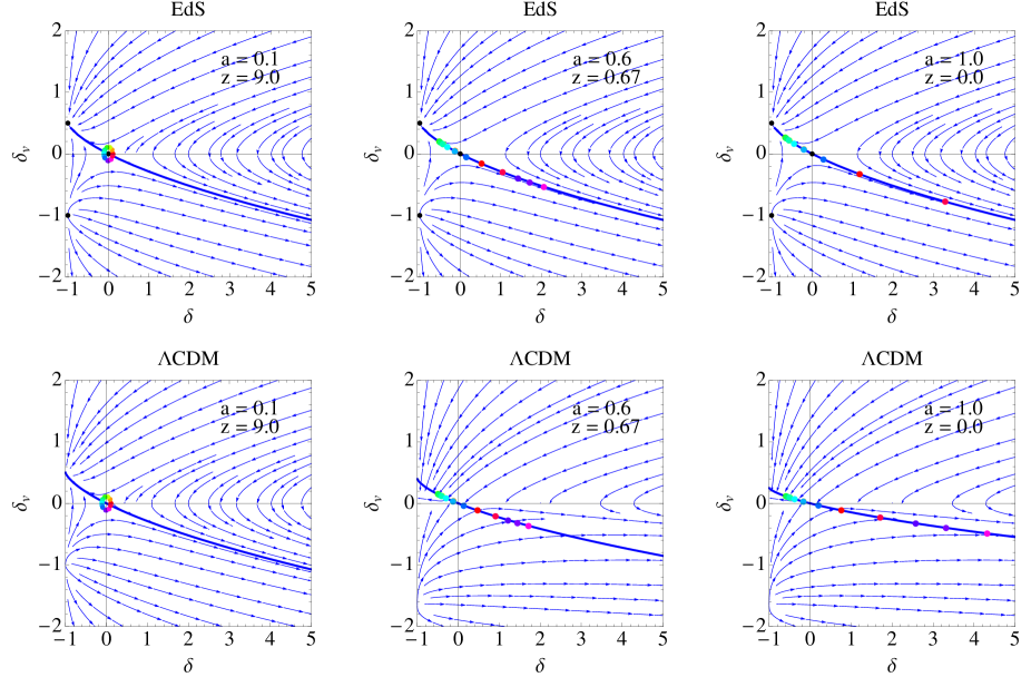
In general, because of the time variation of , the system defined by eqs. (12) and (13) is non-autonomous for dark energy models and techniques of linear stability analysis that are usually performed on autonomous systems are not applicable. However, it is instructive to first consider the EdS case for which the temporal dependence drops and the system becomes autonomous. Figure 3 shows the phase portrait for the two qualitatively different cases: EdS (upper panel) and CDM (lower panel) at three different epochs corresponding to redshifts respectively. The blue lines with arrows are the streamlines of the flow. A streamline is drawn such that the tangent at any point gives the direction of the phase space velocity vector at that point. It denotes the instantaneous direction of evolution of the system. For an autonomous system, the velocity vector is independent of time and the pattern of streamlines is the same at all epochs. However, for a non-autonomous system, the phase space velocity has a time dependence and hence the pattern of streamlines changes with .
For the EdS case, the system has three fixed points, shown by the black dots, at and . The saddle point at the origin corresponds to a unperturbed cosmology, the unstable node at corresponds to a vacuum static model and the attracting point at corresponds to a expanding void model. The solid blue curve is the Zel’dovich curve. The multi-coloured ring of points at corresponds to initial conditions with different values of and , all at a distance of from the centre. Some are very close to the Zel’dovich curve at the start, but others are off the curve. However, as the flow proceeds, all the points evolve to lie close to the Zel’dovich curve at and . The relative deviations from the curve are estimated as , where at a given value of , is the value evolved from initial conditions at and is the value given by the definition of the Zel’dovich curve. The closeness to the curve is characterised by the maximum relative deviation over the points considered for the evolution. Thirteen points were considered and the maximum relative deviation was 14% at and 3% at . The deviation decreases with time indicating that the trajectories asymptotically approach the curve. A point that starts along the curve at was found to remain along the curve with a maximum relative deviation of over the entire range of evolution from to . Thus, the Zel’dovich curve forms an invariant set and acts like an attracting solution for the system.
For the CDM case, at , and . Hence the flow pattern resembles that of the EdS cosmology and the Zel’dovich curves of the two cases are coincident. But as was discussed in the previous section, the Zel’dovich curve evolves with time. It is possible to discuss the stability of such non-autonomous flows in more formal terms using tools from dynamical systems theory (for e.g. Shadden, Lekien, & Marsden 2005), but for the purposes of this paper, we will simply illustrate the ‘attracting’ behaviour of the Zel’dovich curve. We consider the same set of initial conditions, represented by the multi-coloured ring , and evolve them using eqs. (12) and (13). At and at the set has evolved to lie close the corresponding Zel’dovich curves at that epoch. The maximum relative deviations from the corresponding Zel’dovich curve were defined similar to the earlier case, but at fixed instead of . The maximum relative deviation was 17% at and 6% at , again indicating that the Zel’dovich curve acts like an attractor. A point that starts along the curve at stays along it with a maximum relative deviation of over the entire range of evolution. Hence, even in the CDM case, initial conditions that satisfy the Zel’dovich relation at the start continue to maintain it and those that do not, evolve such that they establish it.
Thus, the Zel’dovich curve has a special significance in the dynamics of the perturbations as they evolve in phase space. It gives the long term behaviour of the density and velocity perturbations and is the exact non-linear extension of the density-velocity divergence relation for the spherical top-hat. In the next section we will see that a generalisation of existing formulae by B92 and BCO8 provide a 3% accurate fit to this curve. In figure 3 the deviations from the Zel’dovich curve of the evolved points was greater than this accuracy and one may argue that the fitting forms cannot be useful approximation of the dynamics. However, the initial values of and the ring of radius 0.11 were chosen merely for the sake of convenient plotting and to demonstrate the asymptotic behaviour. Real cosmological initial conditions start evolving at recombination () and sense the presence of the Zel’dovich attractor for a longer period of time. We evolved a similar ring of initial points with an amplitude of from to . The maximum relative deviation over the entire range was within 0.01% indicating that the fits in the following section are indeed a good approximation to the dynamics at the percent level.
3 Fitting functions and growth rates
In this section we show that appropriate modifications of already existing formulae provide a good fit for the Zel’dovich curves. The modification effectively changes the linear growth rate to account for the inclusion of dark energy. Using these fits we also obtain an approximate formula for the growth rate in the non-linear regime.
3.1 Generalisation of existing forms

In the past, various formulae have been proposed for the non-linear density-velocity divergence relation and recent paper by Kitaura et al. (2012) gives a nice summary. Amongst them, the fit by B92 is perhaps the simplest because it has the fewest parameters. However, BC08 showed that this formula was inaccurate for empty universes and provided an improved version based on analytic results of the spherical top-hat model. While their fit has a simple form for overdensities, it has a more involved form for voids. We found that a simple combination of the two formulae by B92 and BC08, appropriately modified to account for the dependence provides a good fit for the Zel’dovich curves.
The original 111Note that the definition of in B92 and our differ by a factor of 3; . Similarly, the variable of BC08 is related to our as . The formulae quoted here have taken these differences into account so that a direct comparison is possible. B92 formula is
| (14) |
This formula is expected to be valid in the range . The original BC08 formula is
| (15) |
where
| (16) | |||||
| (17) | |||||
| (18) |
Both the B92 and the BC08 formulae are obtained for pure matter cosmologies. As was shown in §2.2 there is also expected to be a weak dependence. For a given , varies with and this corresponds to a family of curves for each value of . To estimate the joint dependence on and , Zel’dovich curves were obtained for seven different values of in the range to and at eleven epochs in the range to . The range for each curve was restricted to . In the range we chose a generalised form of the B92 formula
| (19) |
The numerical limit of the Zel’dovich curve and the slope of the curve in the regime fixed the two unknowns and .
| (20) | |||||
| (21) |
where
| (22) | |||||
| (23) |
This fit gave a maximum relative error of within the range of the fit. It gave a error in a higher range of values . In this range, a modification of the formula of BC08 for positive provides a better fit with maximum relative error
| (24) |
The linear limit gives
| (25) |
with
| (26) |
The linear growth index is . We compare this new parametrization for the growth index to the widely accepted result of Linder (2005)
| (27) |
For a CDM cosmology Linder’s value of is recovered exactly. For other values in the range , the relative differences are at most 1%. This fit also modifies the void limit () from for the B92 formula to . This limit is often important when fits to simulation results are compared to analytical estimates (for e.g., Bernardeau et al. 1997; Kudlicki et al. 2000). Note that for most reasonable values of , is rather small and the dependence of the B92 formula is almost unchanged. Similarly, the only change to the overdensity formula of BC08 is in the linear growth factor .
Figure 4 compares the unmodified forms of B92 and BC08 (eqs. (14) and (15)) with the fit presented in this paper for the CDM case at . For this comparison, . The left panel compares positive overdensities, the right panel compares voids. Contrary to what BC08 presented in their paper (fig. 5 in BC08), the unmodified B92 fit seems to perform better than the unmodified BC08 even for higher values of . This could be because the value of chosen for the comparison is different ( in BC08 vs. here) and the comparison there was between matter models as opposed to the CDM model here. This contradiction is somewhat resolved when one compares the modified versions. As mentioned earlier, when compared over the entire range of () and epochs (), the modified version of BC08 performed better (3% max. relative error) at higher than the modified B92 (11% max. relative error) and we advocate using the former for the high regime.
How much improvement has been brought about by the modified combined fit ? We found that over the entire range of and the unmodified B92 (BC08) fits are about 11% (10%) accurate whereas the modified, combined version is 3% (marginally better). In this paper, we have assumed spherical symmetry to derive the non-linear relation. As was commented in BC08, better agreement with the spherical system does not guarantee better agreement with the real system. Numerical simulations or other non-linear techniques will be required to give more refined estimates of this relation, nevertheless, the Zel’dovich curve obtained for the spherical system can provide a starting point to analyse the results.
3.2 Non-linear growth rate
The Zel’dovich curve gives the instantaneous location of the perturbations in phase space. It does not directly give information about the rate at which perturbations evolve along the curve. This is encoded in the growth rate, usually defined as . From eq. (12), we see that the growth rate for the spherical system can be expressed as
| (28) |
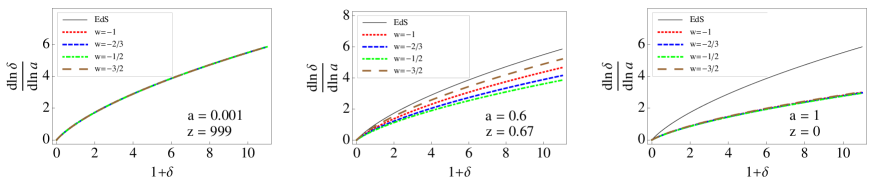
This expression is valid both in the linear and non-linear regimes and we refer to as the total growth rate or non-linear growth rate. Along the Zel’dovich curve, is a function of and the growth rate can be expressed solely as a function of . Figure 5 shows the growth rate vs. along the Zel’dovich curve for different values of at three different redshifts. The colour coding is same as that in figure 2. is a more natural variable than since the former is a measure of the total density of the system. As expected, the growth rate is higher for higher values of ; larger densities grow faster, a signature of gravitational instability. At intermediate epochs, the growth rate is higher for lower values of because the values of are higher (see figure 1). The cumulative effect of higher growth factors can be seen by referring back to figure 3. Consider one of the collapsing perturbations, for example the one shown by the red dot in the upper and lower panels. It starts at the same point in the phase space at for both models. At , it has evolved further along the Zel’dovich curve for the EdS case as opposed to the CDM case. The perturbations shown by the purple and violet dots are already out of the plot at in the upper panel whereas are still at in the lower panel.
Using the fits above, the non-linear growth rate in the regime is
| (29) |
Substituting for and using eqs. (20) and (21) and in the limit of small , we get
| (30) |
To lowest order this reduces to the linear growth rate . At the next order, the non-linear correction is linear in . It would be interesting to check if numerical simulations show a similar dependence of the non-linear growth factor.
4 Connection to observables: Galaxy cluster profiles
Studies of the matter density distribution and pattern of infall velocities around a rich cluster of galaxies have traditionally been used to provide constraints on the matter density (Gunn & Gott 1972; Peebles 1976; Regos & Geller 1989; Willick et al. 1997; Willick & Strauss 1998). More recently, galaxy cluster profiles have also been used as a test of modified gravity (Lombriser et al. 2012). Here we investigate dependence of the cluster density and velocity profiles on the dark energy equation of state. We use the spherical infall model (e.g., Silk & Wilson 1979a; Silk & Wilson 1979b; Villumsen & Davis 1986; Lilje & Lahav 1991, hereafter LL91) to track the evolution of the cluster into the mildly non-linear regime. Our overall set-up is similar to that described in Lahav et al. (1991).
4.1 Equations for spherical infall
The initial configuration of the system is similar to that of the top-hat, but with a radial density variation and hence the perturbation cannot be described by a purely time dependent scale factor. The detailed description of the system and derivation of the relevant equations is given in Appendix A. Here we state the main results. The system is described by a continuum of shells with Lagrangian coordinates , where is the initial physical radius of the shell. The radius of the shell at any later time
| (31) |
The initial perturbation is completely specified by its initial density and velocity profiles. Equations (2) and (3) generalise to
and the evolution of is given by
| (32) |
with initial conditions , and
| (33) |
where the spherically averaged density inside any general radius ‘r’ is given by
| (34) |
The Jacobian that relates the initial Lagrangian and the physical coordinates is
| (35) |
and the density at any later time is
| (36) |
Note that the evolution of is different from that given by eq. (8) due to the spatial dependence of the perturbation scale factor and the combination no longer satisfies the Zel’dovich relation. Instead the relevant quantity is the average density . Substituting eq. (31) in eq. (34) and using the relations eqs. (33), (35) and (36) gives
| (37) |
Comparing eqs. (32) and (37) with eqs. (4) and (8), it is clear that the role played by in the uniform density case is now played by . Physically, this is expected because the velocity is set by the net mass inside the shell. The velocity divergence parameter is similar to eq. (9), but with a spatial dependence
| (38) |
The Zel’dovich curve becomes a relation.
4.2 Initial conditions
The initial density profile was chosen according to the prescription described in LL91 with some minor modifications. This prescription uses the theoretical framework of Bardeen et al. (1986) to predict the density profile around a primordial density peak that nucleates a cluster. The cosmological parameters today were set as , , km. The r.m.s. fluctuation on , , fixed the normalisation of the initial power spectrum. We ran two sets of runs with and . In each set, three equation of state parameters were considered: . The linear density profile today was chosen to be the same for all three cases and the initial profiles at are obtained by multiplying by the appropriate linear growth rate factor. Therefore, the amplitude of the initial density profile was different for the three cases. The initial velocity profile was determined by imposing the linear Zel’dovich condition in the phase space: .
Equation (32) for was integrated numerically for a discrete set of shells from the initial time to the final time . During the course of evolution if , the shell is considered to have collapsed, and forms a part of the cluster core 222Ideally, for collisionless infall, a shell that collapses, bounces back and forth before eventually settling down to a periodic bouncing motion with maximum radius equal to 0.8 times its turnaround radius (Bertschinger 1985). In this case, the shell will collide with outer shells that are undergoing their initial collapse and the equations of motion will be differ from eq. (32). In this paper we follow Lahav et al. (1991) and ignore these effects of secondary infall.. The initial set up is such that the inner shells collapse before the outer shells and no shell crossing takes place anywhere other than at the centre. Further details regarding the initial set-up can be found in Appendix C. In the entire discussion, we assume that light traces matter exactly i.e., the bias factor between galaxies and dark matter is unity. The final density profile is computed using eq. (36) and the final infall velocity is
| (39) |
and are related as
| (40) |
4.3 Results
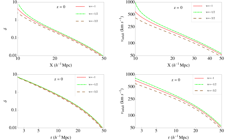
Figure 6 shows the final evolved density and infall velocity profiles at for three cases: (red, dotted), (green, dotdashed) and (brown, long dashed). The runs here correspond to initial conditions with . The plots in the upper panel are drawn against the Lagrangian coordinate () and those in the bottom panel are drawn against the physical distance from the cluster centre (). In the upper panel, the differences in evolution for different models become apparent in the non-linear regime and the curves merge in the linear regime. This is because the linear theory power is fixed to be the same in all models at . Consequently, the amplitude of the initial profile at recombination is higher for higher models because the growth factors are smaller and hence the final non-linear amplitude is more in these models. This is in qualitative agreement with results of McDonald, Trac, & Contaldi (2006), who examined the effect of on the matter power spectrum. The sensitivity to is almost eliminated when the curves are plotted against the physical radius . In the absence of perturbations, the physical radius is just the comoving radius multiplied by the expansion factor . For collapsing perturbations the net physical radius is always less than this; the higher the density and infall velocity, the more tightly bound the system. This causes a bunching of the curves when plotted against .
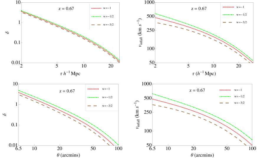
The situation is not too different at higher redshifts. At higher redshifts the distance from the cluster centre (metric separation) is not the relevant observable and is replaced by the angular separation . For a flat universe, the two are related as
| (41) |
is the comoving distance to the object defined as
| (42) |
where is given by eq. (5) and is the speed of light. Figure 7 shows the density and infall velocity patterns at plotted against the metric separation (top panel) and the angular separation (bottom panel). At this redshift, for the fiducial CDM model, eq. (41) reduces to . As was the case at , the density and velocity profiles when plotted against the metric separation, are not too sensitive to the change in . But the angular separation also depends on . For the same metric separation, higher implies a larger angular distance. This broadens the curves and marginally improves the sensitivity to the equation of state parameter especially in the outer regions of the cluster. The redshift is chosen as a typical value in the range . In this range the Zel’dovich curves for different have the maximum spread (see figure 2) and in the next section we show that they can be exploited to remove degeneracies due to parameters such as .
Determination of individual peculiar velocities requires having redshift independent distance measures. Such measures, for e.g., the Tully-Fisher relation (Tully & Fisher 1977), are applicable only to low redshifts (). At these redshifts, they give errors on the order of 100-150 km (e.g., Davis et al. 2011) making it practically impossible to make any reliable estimates at high redshifts, where the error will be worse. Type Ia supernovae may be the best bet to determine individual peculiar velocities at high redshifts, but even these methods have been restricted to low redshifts (for e.g., in Turnbull et al. 2012). Currently and in the near future only statistical information about high redshift peculiar velocity fields will be available via redshift space distortions .
4.4 Parameter degeneracies and the phase space picture

The theoretically predicted profiles in figure 7 were obtained using fixed values of input parameters such as (chosen to be 0.8). Determination of has its own observational uncertainties which introduces a degeneracy between and . Thus, using only the density or only the velocity information cannot not constrain uniquely. We demonstrate that, at redshifts , this degeneracy can be removed by combining the density and velocity information by plotting it on the phase space plot.
Figure 8 shows two sets of average density and velocity profiles and the phase space portrait at . The lower blue set corresponds to with (dotted) and (dashed) and the upper red set is for with the same values. The velocity profiles for almost coincide with . The same is true for the averaged density . But, when the velocity information is combined with the density information and plotted on the phase space portrait, the and points clearly separate and practically lie on their corresponding Zel’dovich curves. The relative deviation from the Zel’dovich curve was calculated for all four sets of points and the maximum over all the points was .
The attracting nature of the Zel’dovich curve ensures small uncertainties in the initial conditions do not affect the final state of the perturbations. Therefore, any degeneracy parameter that affects the initial conditions but not the evolution equations can be eliminated by plotting the density and velocity information on the phase space portrait. Theoretically, this will work best at redshifts near where the spread in the Zel’dovich curves for is maximum. Unfortunately, as was discussed earlier, isolating peculiar velocities at such a high redshift is an extremely challenging task. In addition, degeneracy parameters such as galaxy bias, which arise from observational constraints, cannot be eliminated by this plot.
5 Summary and conclusion
We have obtained the non-linear density-velocity divergence relation by examining the dynamics of perturbations in the joint phase space. Although we were restricted to spherical top-hat models, unlike standard practice, we did not use exact solutions of the top-hat in our derivation of the result. Instead, at each epoch we obtained pairs of initial which satisfied the condition ‘no perturbations at the big bang’. These pairs traced out a curve in the phase space which we refer to as the ‘Zel’dovich curve’. Because of the non-autonomous nature of the evolution equations, this curve is a time dependent entity. We demonstrated that the curve acts like an ‘attractor’ for the dynamics of the perturbations. Small amplitude perturbations, as they evolve through the phase space, asymptotically approach this curve and perturbations that start along the curve stay along it with a very high accuracy. Thus, the Zel’dovich curve gives the long term behaviour of density and velocity perturbations and is exact non-linear extension of the density-velocity curve for the spherical top-hat.
We obtained a 3% fit to the Zel’dovich curve in the range by generalising existing formulae of B92 and BC08 to account for the inclusion of dark energy. From this we obtained a new parametrization for the linear growth index , which agrees with the well known result of Linder (2005) for CDM models and deviates by at most for values of between . As expected, the explicit dependence of the relation on is weak, both in the linear regime and in the non-linear regime. Nevertheless there is a implicit dependence on through the evolution of .
As a practical application, we considered the evolution of density and velocity profiles of galaxies in the quasi-linear regime (), before effects of virialization become important, and investigated the dependence on . We found that the deviations in cluster profiles due to a 50% change in are about km/s which are barely within the current observational errors in the local universe (Courtois & Tully 2012, Davis et al. 2011). We also demonstrated that the degeneracy in the density and velocity profiles arising due to parameters such as can be broken if the same information is plotted on the plot. The attracting behaviour of the Zel’dovich curve makes it insensitive to small changes in the initial parameters and the points get classified according to . However, this is works best only at redshifts , where the curves for different have the maximum spread. Given the observational difficulties in isolating peculiar velocities at these redshifts, this result probably is only of theoretical value at the moment.
The main new feature of this work is the interpretation of the non-linear density-velocity divergence relation in the phase space picture and the generality of the method. In this paper we focussed only on the simplest possible phenomenological model for dark energy: constant equation of state, not necessarily . It would be interesting to consider more generalised models such as varying equation of state, coupled dark energy models or alternate models of gravity. Spherical collapse models have already been worked out for various dark energy or quintessence models (for e.g., Mota & van de Bruck 2004; Maor 2007; Pace et al. 2010) and modified gravity scenarios (for e.g., Dai, Maor, & Starkman 2008; Schäfer & Koyama 2008). The general method remains the same: obtain the correct equation for the evolution of the scale factor, impose the ‘equal age’ condition to get constrains on the initial density and velocity parameters and examine the behaviour of the resulting curve in the phase space dynamics. However several potential caveats and questions may arise. For example in modified gravity scenarios the evolution of a spherical shell enclosing a fixed mass is not independent of the internal distribution of the mass or the environment; Birkoff’s theorem does not hold true and spherical top-hats do not remain top-hats as the evolution proceeds (Dai et al. 2008; Borisov, Jain, & Zhang 2012). Clearly the relation will have to be generalised to treat such situations. It remains to be investigated whether there exist variables related to density and velocity that satisfy a unique relation in phase-space. Recent simulations (Schmidt et al. 2009; Lombriser et al. 2012) have shown that halo density profiles calculated in models of modified gravity show an enhancement at a few virial radii when compared to those evaluated with ‘standard’ CDM. It would be interesting to investigate if the these features translate to a signature in some appropriate Zel’dovich relation.
The Zel’dovich curves were obtained using a spherical top-hat model. In truly inhomogenous systems, the relation is no longer one to one and the joint probability distribution of the two variables provides a more complete description. Whether or not the Zel’dovich relation is obeyed even in a spherically averaged sense is not yet examined. Numerical simulations will be required to give more refined theoretical answers. From an observational point of view too, there are many sources of deviation from spherical symmetry; tidal interactions give rise to transverse forces, infall of smaller systems superimposes a random velocity on the radial infall (e.g., Diaferio & Geller 1997) etc. In addition to the difficulties associated with isolating peculiar velocities, these pose further constraints on the application of the Zel’dovich relation to real systems. Nevertheless, the Zel’dovich curve can provide a pivot point to analyse more complicated systems and we hope that its significance in the density-velocity phase space dynamics can be exploited to constrain cosmological parameters in the future.
Acknowledgements
I would like to thank David F. Chernoff for helpful discussions as well as feedback on the paper and Martha Haynes, the ExtraGalactic Group at Cornell University, J.K. Bhattacharjee, Eanna Flanagan, Rachel Bean, Valeria Pettorino and Shubabrata Majumdar for useful conversations. In addition, I would like to thank Maciej Bilicki for suggestions and valuable comments on the manuscript.
References
- Abramo et al. (2007) Abramo L. R., Batista R. C., Liberato L., Rosenfeld R., 2007, Journal of Cosmology and Astro-Particle Physics, 11, 012
- Allen et al. (2011) Allen S. W., Evrard A. E., Mantz A. B., 2011, Annual Review of Astronomy and Astrophysics, 49, 409
- Bardeen et al. (1986) Bardeen J. M., Bond J. R., Kaiser N., Szalay A. S., 1986, The Astrophysical Journal, 304, 15
- Bernardeau (1992) Bernardeau F., 1992, The Astrophysical Journal, 390, L61
- Bernardeau et al. (1999) Bernardeau F., Chodorowski M. J., Łokas E. L., Stompor R., Kudlicki A., 1999, Monthly Notices of the Royal Astronomical Society, 309, 543
- Bernardeau & van de Weygaert (1996) Bernardeau F., van de Weygaert R., 1996, Monthly Notices of the Royal Astronomical Society, 279, 693
- Bernardeau et al. (1997) Bernardeau F., van de Weygaert R., Hivon E., Bouchet F. R., 1997, Monthly Notices of the Royal Astronomical Society, 290, 566
- Bertschinger (1985) Bertschinger E., 1985, The Astrophysical Journal Supplement Series, 58, 39
- Bilicki & Chodorowski (2008) Bilicki M., Chodorowski M. J., 2008, Monthly Notices of the Royal Astronomical Society, 391, 1796
- Borisov et al. (2012) Borisov A., Jain B., Zhang P., 2012, Physical Review D, 85, 63518
- Bouchet et al. (1995) Bouchet F. R., Colombi S., Hivon E., Juszkiewicz R., 1995, Astronomy and Astrophysics, 296, 575
- Bueno Belloso et al. (2011) Bueno Belloso A., García-Bellido J., Sapone D., 2011, Journal of Cosmology and Astro-Particle Physics, 10, 010
- Chodorowski & Łokas (1997) Chodorowski M. J., Łokas E. L., 1997, Monthly Notices of the Royal Astronomical Society, 287, 591
- Chodorowski et al. (1998) Chodorowski M. J., Łokas E. L., Pollo A., Nusser A., 1998, Monthly Notices of the Royal Astronomical Society, 300, 1027
- Cieciela̧g et al. (2003) Cieciela̧g P., Chodorowski M. J., Kiraga M., Strauss M. A., Kudlicki A., Bouchet F. R., 2003, Monthly Notices of the Royal Astronomical Society, 339, 641
- Courtois & Tully (2012) Courtois H. M., Tully R. B., 2012, Astron. Nachr., 333, 433
- Dai et al. (2008) Dai D.-C., Maor I., Starkman G., 2008, Physical Review D, 77, 64016
- Davis et al. (2011) Davis M., Nusser A., Masters K. L., Springob C., Huchra J. P., Lemson G., 2011, Monthly Notices of the Royal Astronomical Society, 413, 2906
- Dekel (1994) Dekel A., 1994, Annual Review of Astronomy and Astrophysics, 32, 371
- Dekel et al. (1990) Dekel A., Bertschinger E., Faber S. M., 1990, The Astrophysical Journal, 364, 349
- Diaferio & Geller (1997) Diaferio A., Geller M. J., 1997, The Astrophysical Journal, 481, 633
- Dodelson (2003) Dodelson S., 2003, Modern Cosmology. Academic Press
- Engineer et al. (2000) Engineer S., Kanekar N., Padmanabhan T., 2000, Monthly Notices of the Royal Astronomical Society, 314, 279
- Gramann (1993a) Gramann M., 1993a, The Astrophysical Journal, 405, 449
- Gramann (1993b) Gramann M., 1993b, The Astrophysical Journal Letters, 405, L47
- Gunn & Gott (1972) Gunn J. E., Gott J. R., 1972, The Astrophysical Journal, 176, 1
- Guzzo et al. (2008) Guzzo L. et al., 2008, Nature, 451, 541
- Heath (1977) Heath D. J., 1977, Monthly Notices of the Royal Astronomical Society, 179, 351
- Hogg et al. (2005) Hogg D. W., Eisenstein D. J., Blanton M. R., Bahcall N. A., Brinkmann J., Gunn J. E., Schneider D. P., 2005, The Astrophysical Journal, 624, 54
- Kitaura et al. (2012) Kitaura F.-S., Angulo R. E., Hoffman Y., Gottlöber S., 2012, Monthly Notices of the Royal Astronomical Society, 425, 2422
- Komatsu et al. (2011) Komatsu E. et al., 2011, The Astrophysical Journal Supplement Series, 192, 18
- Kowalski et al. (2008) Kowalski M. et al., 2008, The Astrophysical Journal, 686, 749
- Kudlicki et al. (2000) Kudlicki A., Chodorowski M., Plewa T., Różyczka M., 2000, Monthly Notices of the Royal Astronomical Society, 316, 464
- Lahav et al. (1991) Lahav O., Lilje P. B., Primack J. R., Rees M. J., 1991, Monthly Notices of the Royal Astronomical Society, 251, 128
- Lee & Ng (2010) Lee S., Ng K.-W., 2010, Journal of Cosmology and Astro-Particle Physics, 10, 028
- Lilje & Lahav (1991) Lilje P. B., Lahav O., 1991, The Astrophysical Journal, 374, 29
- Lima et al. (1997) Lima J. A. S., Zanchin V., Brandenberger R., 1997, Monthly Notices of the Royal Astronomical Society, 291, L1
- Linder (2005) Linder E. V., 2005, Physical Review D, 72, 43529
- Lombriser et al. (2012) Lombriser L., Schmidt F., Baldauf T., Mandelbaum R., Seljak U., Smith R. E., 2012, Physical Review D, 85, 102001
- Lue et al. (2004) Lue A., Scoccimarro R., Starkman G. D., 2004, Physical Review D, 69, 124015
- Majerotto et al. (2012) Majerotto E. et al., 2012, Monthly Notices of the Royal Astronomical Society, 424, 1392
- Mancinelli & Yahil (1995) Mancinelli P. J., Yahil A., 1995, The Astrophysical Journal, 452, 75
- Mancinelli et al. (1993) Mancinelli P. J., Yahil A., Canon G., Dekel A., 1993, Cosmic Velocity Fields, Proceedings of the 9th IAP Astrophysics Meeting, Institut d’Astrophysique, Paris, July 12-17, 1993. Edited by Fran ois R. Bouchet and Marc Lachi ze-Rey. Gif-sur-Yvette: Editions Frontieres, 215
- Maor (2007) Maor I., 2007, International Journal of Theoretical Physics, 46, 2274
- Martel (1991) Martel H., 1991, The Astrophysical Journal, 377, 7
- McDonald et al. (2006) McDonald P., Trac H., Contaldi C., 2006, Monthly Notices of the Royal Astronomical Society, 366, 547–556
- Mota & van de Bruck (2004) Mota D. F., van de Bruck C., 2004, Astronomy and Astrophysics, 421, 71
- Nadkarni-Ghosh & Chernoff (2011) Nadkarni-Ghosh S., Chernoff D. F., 2011, Monthly Notices of the Royal Astronomical Society, 410, 1454
- Nusser et al. (2012) Nusser A., Branchini E., Davis M., 2012, The Astrophysical Journal, 744, 193
- Nusser & Colberg (1998) Nusser A., Colberg J. M., 1998, Monthly Notices of the Royal Astronomical Society, 294, 457
- Nusser et al. (1991) Nusser A., Dekel A., Bertschinger E., Blumenthal G. R., 1991, The Astrophysical Journal, 379, 6
- Pace et al. (2010) Pace F., Waizmann J.-C., Bartelmann M., 2010, Monthly Notices of the Royal Astronomical Society, 406, 1865–1874
- Peebles (1980) Peebles P., 1980, The Large-Scale Structure of the Universe. Princeton University Press
- Peebles (1976) Peebles P. J. E., 1976, The Astrophysical Journal, 205, 318
- Percival (2005) Percival W. J., 2005, Astronomy and Astrophysics, 443, 819–830
- Regos & Geller (1989) Regos E., Geller M. J., 1989, The Astronomical Journal, 98, 755
- Sarkar et al. (2009) Sarkar P., Yadav J., Pandey B., Bharadwaj S., 2009, Monthly Notices of the Royal Astronomical Society, 399, L128
- Schäfer & Koyama (2008) Schäfer B. M., Koyama K., 2008, Monthly Notices of the Royal Astronomical Society, 385, 411
- Schmidt et al. (2009) Schmidt F., Lima M., Oyaizu H., Hu W., 2009, Physical Review D, 79, 83518
- Scrimgeour et al. (2012) Scrimgeour M. I. et al., 2012, Monthly Notices of the Royal Astronomical Society, 425, 116
- Shadden et al. (2005) Shadden S. C., Lekien F., Marsden J. E., 2005, Physica D Nonlinear Phenomena, 212, 271
- Shaw & Mota (2008) Shaw D. J., Mota D. F., 2008, The Astrophysical Journal Supplement Series, 174, 277
- Silk & Wilson (1979a) Silk J., Wilson M. L., 1979a, The Astrophysical Journal, 228, 641
- Silk & Wilson (1979b) Silk J., Wilson M. L., 1979b, The Astrophysical Journal, 233, 769
- Strauss & Willick (1995) Strauss M. A., Willick J. A., 1995, Physics Reports, 261, 271
- Tully & Fisher (1977) Tully R. B., Fisher J. R., 1977, Astronomy and Astrophysics, 54, 661
- Turnbull et al. (2012) Turnbull S. J., Hudson M. J., Feldman H. A., Hicken M., Kirshner R. P., Watkins R., 2012, Monthly Notices of the Royal Astronomical Society, 420, 447
- Villumsen & Davis (1986) Villumsen J. V., Davis M., 1986, The Astrophysical Journal, 308, 499
- Wang & Steinhardt (1998) Wang L., Steinhardt P. J., 1998, The Astrophysical Journal, 508, 483
- Willick & Strauss (1998) Willick J. A., Strauss M. A., 1998, The Astrophysical Journal, 507, 64
- Willick et al. (1997) Willick J. A., Strauss M. A., Dekel A., Kolatt T., 1997, The Astrophysical Journal, 486, 629
- Wintergerst & Pettorino (2010) Wintergerst N., Pettorino V., 2010, Physical Review D, 82, 103516
- Zel’Dovich (1970) Zel’Dovich Y. B., 1970, Astronomy and Astrophysics, 5, 84
Appendix A Evolution equations for the spherical profile
This appendix gives the equations that govern the evolution of a spherically symmetric matter perturbation in a background cosmology comprising of dark matter and dark energy described by a constant equation of state . Dark energy is not coupled to dark matter and is assumed to stay spatially uniform. The equations derived here hold for perturbations with arbitrary radial density and velocity profiles. The spherical top-hat of §2 becomes a special case.
The physical configuration of the compensated spherical perturbation consists of an inner sphere surrounded by a compensating spherical shell. The background extends beyond the outer edge of the compensating shell. The density in the compensating shell is adjusted so that the mean density of the total mass enclosed within the perturbation is the same as that of the background. Let () denote the density of the background (perturbation). The origin is at the centre of the inner sphere and and denote the physical and comoving distance from the centre.
We start with the generalised Euler equation for the evolution of the velocity (Lima et al. 1997; Abramo et al. 2007; Pace et al. 2010)
| (43) | |||||
| (44) |
where is the comoving coordinate, , is the peculiar gravitational potential and is the matter density perturbation. There are two main frameworks to describe the evolution of a fluid: Eulerian and Lagrangian. In the Eulerian description, one generally solves eq. (43) for as a function of some fixed grid coordinates, whereas in the Lagrangian description, the position is the main variable and is solved as a function of some initial coordinates and time. Since the main aim is to solve for the scale factor, the latter approach is more convenient. Combining the first two terms into a total derivative (), using spherical symmetry and changing to physical radial coordinates , eqs. (43) and (44) become
| (45) | |||||
| (46) |
where the dot is derivative w.r.t. time and the background scale factor evolves as
| (47) |
Define the Lagrangian coordinate of a shell as the initial comoving coordinate of the shell i.e., . The physical radius of any shell at a later time can be written as
| (48) |
where can be thought of as the scale factor of the shell at . By definition . The perturbation is described by two quantities: initial overdensity parameter
| (49) |
and the velocity perturbation parameter
| (50) |
where and are the initial total velocity and initial total density profiles of the perturbation and is the initial total density of the background. Conservation of mass implies that the matter density at any later time
| (51) |
where is the Jacobian factor relating the Eulerian and Lagrangian volume elements,
| (52) |
Using eq. (48),
| (53) |
By construction,
| (54) |
The background density and using eqs. (49), (51) and (54) the perturbed density evolves as
| (55) |
From spherical symmetry, the force
| (56) |
Convert to Lagrangian coordinates by substituting eqs. (48), (52) and (55) in (56)
| (57) |
Define
| (58) |
is the average fractional density of mass within radius . Substituting eqs. (48) and (57) in eq. (45), setting and using eq. (47) for the evolution of the background gives
| (59) |
The initial conditions are and .
If the initial density is uniform, and and the dependence drops out of the equation for evolution of . An initially uniform spherical perturbation continues to stay uniform and can be described by .
| (60) |
with initial conditions and . This equation is similar to many others stated more directly in the literature (see for e.g., Percival 2005). Here we use the route advocated in recent papers (Pace et al. 2010; Wintergerst & Pettorino 2010) so that the set up can be generalised to cases where dark energy may have more complicated behaviour.
In the above derivation we have assumed that the Lagrangian system is a good coordinate system to describe the evolution. This is true as long as no shell crossing occurs within the system, which ensures that the mapping between the physical coordinates and the Lagrangian coordinates is unique. For the top-hat case, the argument that supports this assumption is presented in Appendix A of NC. Here we extend it to the spherical infall model. Let be the initial physical distance of the edge of the cluster from the center. The velocity of the edge is . Given the perturbation parameters and , one can always choose (and hence ) arbitrarily small so that the time for the edge to reach any physical distance is arbitrarily large. The initial density is maximum at the center and decreases monotonically as increases (see Appendix C for the initial set-up). The velocity perturbation is proportional to , but with a negative sign and hence increases as one moves from the center to the edge. Thus, the net gravitational binding is tighter near the cluster center than the edge. This ensures that a shell initially closer to the center does not cross any shell at a greater initial radius and collapses into the center earlier. The choice of the edge radius fixes the net mass inside. The additional mass needed to satisfy mass conservation is put in a compensating shell between the cluster edge and the inner edge of the background and set on a critical trajectory outward so that it moves along with the background.
Appendix B Time dependence of the Zel’dovich condition for dark energy
The evolution of the background and perturbation scale factors for the top-hat perturbation is given by
| (61) | |||||
| (62) |
where are the Hubble parameter and density parameters at the initial time and are related to their values today () through
| (63) | |||||
| (64) |
The initial conditions are , , and . Substitute ,, in eqs. (61) and (62). The two equations then read
| (65) | |||||
| (66) |
with initial conditions , , , . Note that the equal age condition is unchanged by this scaling since the time is scaled by the same constant both for the background and perturbation. It is also clear that the equal age condition will only involve the parameters and . For a flat EdS universe and at all times. Equations (65) and (66) can be integrated to give
| (67) |
The age of the background (perturbation) is the time elapsed for to grow from 0 to 1. Imposing the ‘equal age’ condition, gives an implicit relation between and
| (68) |
In the presence of a dark energy term analytic calculations are not possible. For such cases, given a and at , the age of the perturbation can be computed by integrating eq. (66) back in time until reaches zero. Fixing one performs a search in the parameter space until the age of the background and perturbation are the same. However for models with , an additional complication arises because eq. (66) has a singularity when . This condition is independent of and can complicate the search. So, instead of backward integration, we set at the big bang time (epoch when ) and integrate forward in time until . The time elapsed gives the age of the perturbation. A search is performed to find the velocity at the bang time for which the ages of the background and perturbation are the same. The initial velocity at can be read off from the solution: .
Appendix C Setting the initial density profile of cluster progenitors
The initial density and velocity profiles are set, as per the prescription in LL91, with some minor modifications. This paper uses results from the BBKS (Bardeen et al. 1986) analysis. The basic premise is that matter collapses around the peaks in the primordial density field, filtered on some appropriate length scale, forming the progenitors of bound cosmic structures.
Start with the CDM power spectrum , where the transfer function has the BBKS form (Bardeen et al. 1986)
| (69) | |||||
| (70) |
is measured in . The spectral index was chosen, in accordance with LL91 to have the Harrison-Zel’dovich value , which is slightly higher than the current WMAP ‘standard’ value from seven year observations (Komatsu et al. 2011). The normalisation is set by demanding that the r.m.s. fluctuation on 8 Mpc () defined as
| (71) |
where , matches the observed value. We ran separate cases with two values and . The normalised power spectrum is filtered with a Gaussian filter of width
| (72) |
where
| (73) |
The height of any peak in the density distribution is usually denoted as where is the r.m.s. of the filtered density field. The ensemble average of the radial distribution of the density field around a peak of relative height is given by
| (74) |
Here and are spectral parameters and is a function of and (see LL91).
The fractional peak height is a random variable with a comoving differential number density and ideally one must evolve many initial profiles with different values of drawn from this distribution. Instead, we follow LL91 and substitute for and in eq. (74) the average values and
| (75) |
where the threshold is the peak height above which clusters can form. This is set by requiring that the theoretical number density of galaxy clusters above the threshold equals the observed number density .
| (76) |
We use for clusters with mass greater than (Allen, Evrard, & Mantz 2011).
The function set up by this method corresponds to the linear profile at . This is transformed into the profile at any other redshift by multiplying by the appropriate growth factor.
| (77) |
where the growth factor is (Heath 1977; Dodelson 2003)
| (78) |
This expression for the growth factor has been derived for pressureless matter universes, but is also valid for dark energy cosmologies described by constant . §4.1 sets up the initial profile in terms of Lagrangian coordinates: . The initial profiles are chosen so that at the linear theory profile is same in all models. Since the growth factor is different for different , the initial profiles have different amplitudes; higher values have slower growth i.e., is smaller and hence a larger initial amplitude. The initial average density perturbation inside a radius is
| (79) |
The velocity perturbation is chosen by imposing Zel’dovich initial conditions
| (80) |
At recombination, for all values of . Note that the definition of slightly differs from a similar velocity perturbation parameter defined in LL91.