Laplace deconvolution and its application to Dynamic Contrast Enhanced imaging

Abstract

In the present paper we consider the problem of Laplace deconvolution with noisy discrete observations. The study is motivated by Dynamic Contrast Enhanced imaging using a bolus of contrast agent, a procedure which allows considerable improvement in evaluating the quality of a vascular network and its permeability and is widely used in medical assessment of brain flows or cancerous tumors. Although the study is motivated by medical imaging application, we obtain a solution of a general problem of Laplace deconvolution based on noisy data which appears in many different contexts. We propose a new method for Laplace deconvolution which is based on expansions of the convolution kernel, the unknown function and the observed signal over Laguerre functions basis. The expansion results in a small system of linear equations with the matrix of the system being triangular and Toeplitz. The number $m$ of the terms in the expansion of the estimator is controlled via complexity penalty. The advantage of this methodology is that it leads to very fast computations, does not require exact knowledge of the kernel and produces no boundary effects due to extension at zero and cut-off at $T$. The technique leads to an estimator with the risk within a logarithmic factor of $m$ of the oracle risk under no assumptions on the model and within a constant factor of the oracle risk under mild assumptions. The methodology is illustrated by a finite sample simulation study which includes an example of the kernel obtained in the real life DCE experiments. Simulations confirm that the proposed technique is fast, efficient, accurate, usable from a practical point of view and competitive.

AMS 2010 subject classifications. 62G05, 62G20, 62P10.
Key words and phrases: Laplace deconvolution, complexity penalty, Dynamic Contrast Enhanced imaging

1 Introduction

Cancers and vascular diseases present major public health concerns. Considerable improvement in assessing the quality of a vascular network and its permeability have been achieved through Dynamic Contrast Enhanced (DCE) imaging using a bolus of contrast agent at high frequency such as Dynamic Contrast Enhanced Computer Tomography (DCE-CT), Dynamic Contrast Enhanced Magnetic Resonance Imaging (DCE-MRI) and Dynamic Contrast Enhanced Ultra Sound (DCE-US). Such techniques are widely used in medical assessment of brain flows or cancerous tumors (see, e.g., Cao et al., 2010; Goh et al., 2005; Goh and Padhani, 2007; Cuenod et al., 2006; Cuenod et al., 2011; Miles, 2003; Padhani and Harvey, 2005 and Bisdas et al., 2007). This imaging procedure has great potential for cancer detection and characterization, as well as for monitoring in vivo the effects of treatments. It is also used, for example, after a stroke for prognostic purposes or for occular blood flow evaluation.

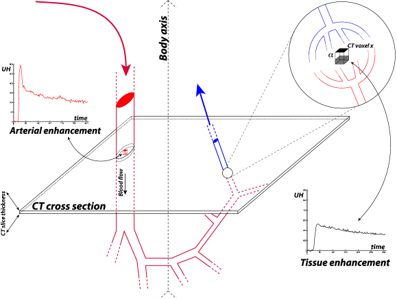
Figure 1: DCE-CT experiment and contrast agent circulation. The patient body is materialized by the mixed arrow.

As an example, below we consider a DCE-CT experiment that follows the diffusion of a bolus of a contrast agent injected into a vein. At the microscopic level, for a given voxel of interest having unit volume, the number of arriving particles at time $t$ is given by $\beta\,\mbox{AIF}(t)$, where the Arterial Input Function (AIF) measures concentration within a unit volume voxel inside the aorta and $\beta$ is a proportion of the AIF which enters the tissue voxel. Denote the number of particles in the voxel at time $t$ by $Y(t)$ and the random lapse of time during which a particle sojourns in the voxel by $S$. Assuming sojourn times for different particles to be i.i.d. with c.d.f. $F$, one obtains the following equation for the average number of contrast agent particles at the moment $t$

$${{\mathbb{E}}}Y(t)=\underbrace{\int_{0}^{t}\beta\,\mbox{AIF}(t-\tau)\,d\tau}_{\text{arrived before time $t$}}-\underbrace{\int_{0}^{t}\beta\,\mbox{AIF}(t-\tau)\,P(S\leq\tau)\,d\tau}_{\text{left before time $t$}}=\int_{0}^{t}\beta\,\mbox{AIF}(t-\tau)(1-F(\tau))d\tau,$$

where the expectation is taken under the unknown distribution of the sojourn times. In reality, one does not know ${{\mathbb{E}}}Y(t)$ and has discrete noisy observations

$$Y(t_{i})={{\mathbb{E}}}Y(t_{i})+\sigma\epsilon_{i}.$$

Medical doctors are interested in a reproducible quantification of the blood flow inside the tissue which is characterized by $f(t)=\beta(1-F(t))$ since this quantity is independent of the concentration of particles of contrast agent within a unit volume voxel inside the aorta described by $\mbox{AIF}(t)$. The sequential imaging acquisition is illustrated by Figure 1. The contrast agent arrives with the oxygenated blood through the aorta (red arrow) where its concentration, AIF, within unit volume voxel is first measured when it passes through the CT cross section (red box). Subsequently, the contrast agent enters the arterial system, and it is assumed that its concentration does not change during this phase. The exchange within the tissue of both oxygen and contrast agent occurs after the arterial phase and the concentration of contrast agent during this exchange is measured in all tissue voxels (grey voxel in the zoom) inside the CT cross section. Later the contrast agent returns to the venous system with the de-oxygenated blood (blue arrow).

To complete description of this experiment, one has to take into account that there is a delay $\delta$ between the measurement of the contrast agent concentration inside the aorta (first cross of the CT section) and its arrival inside the tissue. This leads to the following complete model:

$$Y(t_{i})=\int_{0}^{t_{i}-\delta}\beta\mbox{AIF}(t_{i}-\tau)(1-F(\tau))d\tau+\sigma\epsilon_{i},\;\;\;i=1,...,n.$$ (1.1)

The value of delay $\delta$ can be measured with a small error using the decay between the jumps after the injection of the contrast agent inside the aorta and the tissue. Unfortunately, evaluation of the proportion $\beta$ is a much harder task which is realized with a larger error. In the spirit of complete model (1.1) for DCE-CT experiments, one can consider a more general model of Laplace convolution equation based on noisy observations which presents a necessary theoretical step before obtaining medical answers provided by model (1.1).

Indeed, for a known value of $\delta$, equation (1.1) reduces to a noisy version of a Laplace convolution equation

$$y(t_{i})=\int_{0}^{t_{i}}g(t_{i}-\tau)f(\tau)d\tau+\sigma\epsilon_{i},\;\;\;i=1,\ldots,n,$$ (1.2)

where function $g$ is considered to be known, $f$ is a function of interest, measurements $y(t_{i})$ are taken at points $0\leq t_{1}\leq...\leq t_{n}\leq T<\infty$ and $\epsilon_{i}$ are i.i.d. $N(0,1)$. The corresponding noiseless version of this equation can be written as

$$q(t)=\int_{0}^{t}g(t-\tau)f(\tau)d\tau,\;t\geq 0.$$ (1.3)

Formally, by setting $g(t)=f(t)\equiv 0$ for $t<0$, equation (1.3) can be viewed as a particular case of the Fredholm convolution equation

$$q(t)=\int_{a}^{b}g(t-\tau)f(\tau)d\tau,$$ (1.4)

where $a=-\infty$ and $b=\infty$ for Fourier convolution on a real line and $-\infty<a<b<\infty$ for circular convolution. Discrete stochastic version of equation (1.4)

$$y(t_{i})=\int_{a}^{b}g(t_{i}-\tau)f(\tau)d\tau+\sigma\epsilon_{i},\;\;\;\;i=1,...,n,$$ (1.5)

known also as Fourier deconvolution problem, has been extensively studied in the last thirty years (see, for example, Carroll and Hall, 1988; Comte, Rozenholc and Taupin, 2007; Delaigle, Hall and Meister, 2008; Diggle and Hall, 1993; Fan, 1991; Fan and Koo, 2002; Johnstone et al., 2004; Pensky and Vidakovic, 1999; Stefanski and Carroll, 1990, among others). However, such an approach to solving (1.3) and (1.2) is very misleading.

Indeed, since one does not have data outside the interval $[0,T]$ and since function $f(t)$ may not vanish fast enough as $t\to\infty$, one cannot apply Fourier transform on the whole real line since Fourier transform is defined for only integrable or square integrable functions. Application of the discrete Fourier transform (DFT) on the finite interval $[0,T]$ is useless since the kernel $g$ is not periodic. Consequently, convolution in equation (1.3) is not circular and, hence, it is not converted into a product by DFT.

The issue of having measurements only on the part $t\leq T$ of half line $(0,\infty)$ does not affect the Laplace deconvolution since it exhibits causality property: the values of $q(t)$ for $0\leq t\leq T$ depend on values of $f(t)$ for $0\leq t\leq T$ only and vice versa.

The mathematical theory of (noiseless) convolution type Volterra equations is well developed (see, e.g., Gripenberg et al. 1990) and the exact solution of (1.3) can be obtained through Laplace transform. However, direct application of Laplace transform for discrete measurements faces serious conceptual and numerical problems. The inverse Laplace transform is usually found by application of tables of inverse Laplace transforms, partial fraction decomposition or series expansion (see, e.g., Polyanin and Manzhirov, 1998), neither of which is applicable in the case of the discrete noisy version of Laplace deconvolution. Only few applied mathematicians and researchers in natural sciences took an effort to solve the problem using discrete measurements in the left hand side of (1.4). Since the problem arises in medical imaging, few scientists put an effort to solve equation (1.1) using singular value decomposition (SVD) with the subsequent application of Tikhonov regularization (see, e.g., Axel (1980), Ostergaard et al. (1996) and an extensive review in Fieselmann et al. (2011)). In fact, SVD has been widely used in the context of DCE imaging since mid-nineties. The technique, however, is very computationally unstable, especially, in the presence of recirculation of contrast agent. For this reason, SVD has been mostly used in the simplified framework of brain imaging due to the presence of white barrier which prevents circulation of contrast agent outside blood vessels. Ameloot and Hendrickx (1983) applied Laplace deconvolution for the analysis of fluorescence curves and used a parametric presentation of the solution $f$ as a sum of exponential functions with parameters evaluated by minimizing discrepancy with the right-hand side. In a somewhat similar manner, Maleknejad et al. (2007) proposed to expand the unknown solution over a wavelet basis and find the coefficients via the least squares algorithm. Lien et al. (2008), following Weeks (1966), studied numerical inversion of the Laplace transform using Laguerre functions. Finally, Lamm (1996) and Cinzori and Lamm (2000) used discretization of the equation (1.3) and applied various versions of the Tikhonov regularization technique. However, in all of the above papers, the noise in the measurements was either ignored or treated as deterministic. The presence of random noise in (1.2) makes the problem even more challenging.

For the reasons listed above, estimation of $f$ from discrete noisy observations $y$ in (1.2) requires extensive investigation. Unlike Fourier deconvolution that has been intensively studied in statistical literature (see references above), Laplace deconvolution received very little attention within statistical framework. To the best of our knowledge, the only paper which tackles the problem is Dey, Martin and Ruymgaart (1998) which considers a noisy version of Laplace deconvolution with a very specific kernel of the form $g(t)=be^{-at}$. The authors use the fact that, in this case, the solution of the equation (1.3) satisfies a particular linear differential equation and, hence, can be recovered using $q(t)$ and its derivative $q^{\prime}(t)$. For this particular kind of kernel, the authors derived convergence rates for the quadratic risk of the proposed estimators, as $n$ increases, under the assumption that the $s$-th derivative of $f$ is continuous on $(0,\infty)$. However, in Dey, Martin and Ruymgaart (1998) it is assumed that data are available on the whole positive half-line (i.e. $T=\infty$) and that $s$ is known (i.e., the estimator is not adaptive).

Recently, Abramovich et al. (2012) studied the problem of Laplace deconvolution based on discrete noisy data. The idea of the method is to reduce the problem to estimation of the unknown regression function, its derivatives and, possibly, some linear functionals of these derivatives. The estimation is carried out using kernel method with the Lepskii technique for the choice of the bandwidth (although it is mentioned in the paper that other methodologies for the choice of bandwidth can also be applied). The method has an advantage of reducing a new statistical problem to a well studied one. However, the shortcoming of the technique is that it requires meticulous boundary correction and is strongly dependent on the knowledge of the kernel $g$. Indeed, small change in the kernel may produce significant changes in the expression for the estimator.

In the present paper we suggest a method which is designed to overcome limitations of the previously developed techniques. The new methodology is based on expansions of the kernel, unknown function $f$ and the right-hand side in equation (1.2) over the Laguerre functions basis. The expansion results in a small system of linear equations with the matrix of the system being triangular and Toeplitz. The number of the terms in the expansion of the estimator is controlled via complexity penalty. The advantage of this methodology is that it leads to very fast computations and produces no boundary effects due to extension at zero and cut-off at $T$. The technique does not require exact knowledge of the kernel since it is represented by its Laguerre coefficients only and leads to an estimator with the risk within a logarithmic factor of $m$ of the oracle risk under no assumptions on the model and within a constant factor of the oracle risk under mild assumptions. Another merit of the new methodology includes the fact that, since the unknown functions are represented by a small number of Laguerre coefficients, it is easy to cluster or classify them for various groups of patients. Simulation study shows that the method is very accurate and stable and easily outperforms SVD and kernel-based technique of Abramovich, Pensky, and Rozenholc (2012).

The rest of the paper is organized as follows. In Section 2 we derive the system of equations resulting from expansion of the functions over the Laguerre basis, study the effect of discrete, possible irregularly spaced data and introduce selection of model size via penalization. Corollary 1 indeed confirms that the risk of the penalized estimator lies within a logarithmic factor of $m$ of the minimal risk. In Section 3 we obtain asymptotic upper bounds for the risk and prove the risk lies within a constant factor of an oracle risk. The proof of this fact rests on nontrivial facts of the theory of Toeplitz matrices. Section 4 provides a finite sample simulation studies. Finally, Section 5 discusses results obtained in the paper. Section 6 contains proofs of the results in the earlier sections.

2 Laplace deconvolution via expansion over Laguerre functions basis

2.1 Relations between coefficients of the Laguerre expansion

One of the possible solution of the problem (1.2) is to use Galerkin method with the basis represented by a system of Laguerre functions. Laguerre functions are defined as

$$\phi_{k}(t)=\sqrt{2a}e^{-at}L_{k}(2at),\ \ k=0,1,\ldots,$$ (2.1)

where $L_{k}(t)$ are Laguerre polynomials (see, e.g., Gradshtein and Ryzhik (1980))

$$L_{k}(t)=\sum_{j=0}^{k}(-1)^{j}{k\choose j}\frac{t^{j}}{j!},\ \ \ t\geq 0.$$

It is known that functions $\phi_{k}(\cdot)$, $k=0,1,\ldots$, form an orthonormal basis of the $L^{2}(0,\infty)$ space and, therefore, functions $f(\cdot)$, $g(\cdot)$, $q(\cdot)$ and $y(\cdot)$ can be expanded over this basis with coefficients $f^{(k)}$, $g^{(k)}$, $q^{(k)}$ and $y^{(k)}$, $k=0,\ldots,\infty$, respectively. By plugging these expansions into formula (1.3), we obtain the following equation

$$\sum_{k=0}^{\infty}q^{(k)}\phi_{k}(t)=\sum_{k=0}^{\infty}\sum_{j=0}^{\infty}f^{(k)}g^{(j)}\int_{0}^{t}\phi_{k}(x)\phi_{j}(t-x)dx.$$ (2.2)

It turns out that coefficients of interest $f^{(k)}$, $k=0,1,\ldots,$ can be represented as a solution of an infinite triangular system of linear equations. Indeed, it is easy to check that (see, e.g., 7.411.4 in Gradshtein and Ryzhik (1980))

$$\int_{0}^{t}\phi_{k}(x)\phi_{j}(t-x)dx=2ae^{-at}\int_{0}^{t}L_{k}(2at)L_{j}(2a(t-x))dx=(2a)^{-1/2}\,[\phi_{k+j}(t)-\phi_{k+j+1}(t)].$$

Hence, equation (2.2) can be re-written as

$$\sum_{k=0}^{\infty}q^{(k)}\phi_{k}(t)=\sum_{k=0}^{\infty}\phi_{k}(t)[(2a)^{-1/2}\,f^{(k)}g^{(0)}+\sum_{l=0}^{k-1}(2a)^{-1/2}\,(g^{(k-1)}-g^{(k-l-1)})f^{(l)}].$$

Equating coefficients for each basis function, we obtain an infinite triangular system of linear equations. In order to use this system for estimating $f$, we define

$$f_{m}(x)=\sum_{k=0}^{m-1}{f}^{(k)}\phi_{k}(x),$$ (2.3)

approximation of $f$ based on the first $m$ Laguerre functions. The following Lemma states how the coefficients in (2.3) can be recovered.

Lemma 1.

Let $\mbox{\boldmath$f$}_{m}$, $\mbox{\boldmath$g$}_{m}$ and $\mbox{\boldmath$q$}_{m}$ be $m$-dimensional vectors with elements $f^{(k)}$, $g^{(k)}$ and $q^{(k)}$, $k=0,1,\ldots,m-1$, respectively. Then, for any $m$, one has $\mbox{\boldmath$q$}_{m}=\mbox{\boldmath$G$}_{m}\mbox{\boldmath$f$}_{m}$ where $\mbox{\boldmath$G$}_{m}$ is the lower triangular Toeplitz matrix with elements

$$G^{(i,j)}=\left\{\begin{array}[]{ll}(2a)^{-1/2}\,g^{(0)},&\mbox{if}\ \ i=j,\\ (2a)^{-1/2}\,(g^{(i-j)}-g^{(i-j-1)}),&\mbox{if}\ \ j<i,\\ 0,&\mbox{if}\ \ j>i.\end{array}\right.$$ (2.4)

Hence, $f(x)$ can be estimated by

$$\hat{f}_{m}(x)=\sum_{k=0}^{m-1}\hat{f}^{(k)}\phi_{k}(x)$$ (2.5)

where $\hat{\mbox{\boldmath$f$}}_{m}=\mbox{\boldmath$G$}_{m}^{-1}\hat{\mbox{\boldmath$q$}}_{m}$ and $\hat{\mbox{\boldmath$q$}}_{m}$ is an unbiased estimator of the unknown vector of coefficients $\mbox{\boldmath$q$}_{m}$.

2.2 Recovering Laguerre coefficients from discrete noisy data

Unfortunately, unlike some other linear ill-posed problems, data does not come in the form of unbiased estimators of the unknown coefficients $q^{(k)}$, $k=0,1,\ldots,m-1$. Below, we examine how the length of the observation interval $T$ and spacing of observations $t_{i}$ in equation (1.2) affect the system of equations in Lemma 1.

Let $P:[0,T]\rightarrow[0,T]$ be a function generating observations in (1.2) such that $P$ is a continuously differentiable strictly increasing function

$$P(0)=0,\ \ P(T)=T,\ \ P(t_{i})=iT/n,\ \ i=1,\ldots,n.$$ (2.6)

Under conditions (2.6), $P$ is a one-to-one function and, therefore, has an inverse $P^{-1}$.

Choose $M$ large enough that the bias in representation (2.3) of $f$ by $f_{M}$ is very small and form an $(n\times M)$ matrix $\mbox{$\Phi$}_{M}$ with elements $\Phi^{(i,k)}=\phi_{k}(t_{i})$, $i=1,\ldots,n,$ $k=0,\ldots,M-1$. Let $\mbox{\boldmath$z$}_{M}$ be the $M$-dimensional vector with elements $z^{(j)}=\langle y,\phi_{j}\rangle$, $j=0,\ldots,M-1$. Then, it follows that

$$y(t_{i})=\sum_{l=0}^{M-1}z^{(l)}\phi_{l}(t_{i})=(\mbox{$\Phi$}_{M}\mbox{\boldmath$z$}_{M})^{(i)},\ \ i=1,\ldots,n.$$

If $y$ and $h$ are $n$-dimensional vectors with components $y(t_{i})$ and $q(t_{i})$, $i=1,\ldots,n$, respectively, then the vectors $\mbox{\boldmath$q$}_{M}$ and $\mbox{\boldmath$z$}_{M}$ of the true and the estimated Laguerre coefficients of $q(x)$ can be represented, respectively, as

$$\mbox{\boldmath$q$}_{M}=(\mbox{$\Phi$}_{M}^{T}\mbox{$\Phi$}_{M})^{-1}\mbox{$\Phi$}_{M}^{T}\mbox{\boldmath$h$},\ \ \ \mbox{\boldmath$z$}_{M}=(\mbox{$\Phi$}_{M}^{T}\mbox{$\Phi$}_{M})^{-1}\mbox{$\Phi$}_{M}^{T}\mbox{\boldmath$y$}.$$ (2.7)

Let us examine matrix $\mbox{$\Phi$}_{M}^{T}\mbox{$\Phi$}_{M}$. Note that, for any $k$ and $l$,

$$(\mbox{$\Phi$}_{M}^{T}\mbox{$\Phi$}_{M})^{(k,l)} = \sum_{i=1}^{n}\phi_{k}(P^{-1}(iT/n))\phi_{l}(P^{-1}(iT/n))\approx nT^{-1}\,\int_{0}^{T}\phi_{k}(P^{-1}(x))\phi_{l}(P^{-1}(x))dx$$

$$= nT^{-1}\,\int_{0}^{T}\phi_{k}(t)\phi_{l}(t)p(t)dt$$

where $p(t)=P^{\prime}(t)$. It follows from the above that matrix $\mbox{$\Phi$}_{M}^{T}\mbox{$\Phi$}_{M}$ should be normalized by a factor $n^{-1}T$. Indeed, if points $t_{i}$ are equispaced on the interval $(0,T]$, then, for $n$ and $T$ large enough, $(\mbox{$\Phi$}_{M}^{T}\mbox{$\Phi$}_{M})\approx nT^{-1}\,\mbox{\boldmath$I$}_{M}$ where $\mbox{\boldmath$I$}_{M}$ is the $M$-dimensional identity matrix. Hence, in what follows, we are going to operate with matrix $\mbox{\boldmath$A$}_{M}=Tn^{-1}(\mbox{$\Phi$}_{M}^{T}\mbox{$\Phi$}_{M})$ and its inverse

$$\mbox{$\Omega$}_{M}=(\mbox{\boldmath$A$}_{M})^{-1}=nT^{-1}(\mbox{$\Phi$}_{M}^{T}\mbox{$\Phi$}_{M})^{-1}.$$ (2.8)

Let $\epsilon$ be the vector with components $\epsilon(t_{i})$, $i=1,\ldots,n$, and $\mbox{$\xi$}_{M}=\sqrt{n/T}\ (\mbox{$\Phi$}_{M}^{T}\mbox{$\Phi$}_{M})^{-1}\mbox{$\Phi$}_{M}^{T}\mbox{$\epsilon$}$. Then, the vector $\mbox{\boldmath$f$}_{M}$ of the true Laguerre coefficients of the unknown function $f$ satisfies the following equation

$$\mbox{\boldmath$z$}_{M}=\mbox{\boldmath$G$}_{M}\mbox{\boldmath$f$}_{M}+\sigma\sqrt{T/n}\ \mbox{$\xi$}_{M},\ \ \mbox{$\xi$}_{M}\sim N(\mbox{\boldmath$0$},\mbox{$\Omega$}_{M}).$$ (2.9)

If points $t_{i}$ are equispaced on the interval $(0,T]$ and both $n$ and $T$ are large, then, in (2.9), $\mbox{$\Omega$}_{M}\approx\mbox{\boldmath$I$}_{M}$.

2.3 Model selection and oracle risk

Equation (2.9) implies that one can estimate unknown vector $\mbox{\boldmath$f$}_{M}$ by $\hat{\mbox{\boldmath$f$}}_{M}=\mbox{\boldmath$G$}_{M}^{-1}\mbox{\boldmath$z$}_{M}$. However, since the value of $M$ is large, the variance of this estimator,

$${\mathbb{E}}\|\hat{\mbox{\boldmath$f$}}_{M}-\mbox{\boldmath$G$}_{M}^{-1}\mbox{\boldmath$q$}_{M}\|^{2}=\frac{\sigma^{2}T}{n}\,\mbox{Tr}(\mbox{\boldmath$G$}_{M}^{-1}\mbox{$\Omega$}_{M}\mbox{\boldmath$G$}_{M}^{-T}),$$

where $\mbox{\boldmath$A$}^{-T}=(\mbox{\boldmath$A$}^{T})^{-1}=(\mbox{\boldmath$A$}^{-1})^{T}$ for any matrix $A$, will be too large while the bias in the representation (2.3) of $f$ by $f_{M}$ will be very small. Hence, in order to balance the bias and the variance components of the error, one needs to choose the best possible number $m$ of Laguerre functions in the representation (2.3) of $f$, i.e., choose the model size.

In order to achieve a required balance between the bias and the variance components of the error, consider a collection of integer indices ${\mathcal{M}}_{n}=\{1,\ldots,M\}$ where $M<n$ may depend on $n$ and, for $m\in{\mathcal{M}}_{n}$, the associated subspaces $S_{m}\subseteq R^{M}$ defined by

$$\mbox{\boldmath$t$}\in S_{m}\ \ \mbox{if}\ \ \mbox{\boldmath$t$}=(t^{(0)},t^{(1)},\ldots,t^{(m-1)},0,0,\ldots,0)^{T}.$$

Let us denote by $\vec{\mbox{\boldmath$z$}}_{m}$, $\vec{\mbox{\boldmath$q$}}_{m}$, $\vec{\mbox{\boldmath$f$}}_{m}$, $\vec{\mbox{$\xi$}}_{m}$ and $\widehat{\vec{\mbox{\boldmath$f$}}}_{m}$ the $M$-dimensional vectors where the first $m$ elements coincide with the elements of $m$-dimensional vectors $\mbox{\boldmath$z$}_{m}$, $\mbox{\boldmath$q$}_{m}$, $\mbox{\boldmath$f$}_{m}$, $\mbox{$\xi$}_{m}$ and $\widehat{\mbox{\boldmath$f$}}_{m}$ respectively, and the last $(M-m)$ elements are identical zeros. For each $m\in{\mathcal{M}}_{n}$, evaluate

$$\widehat{\mbox{\boldmath$f$}}_{m}=(\mbox{\boldmath$G$}_{m})^{-1}\mbox{\boldmath$z$}_{m}=\mbox{\boldmath$G$}_{M}^{-1}\vec{\mbox{\boldmath$z$}}_{m}$$

and denote

$$\mbox{\boldmath$Q$}_{m}=\mbox{\boldmath$G$}_{m}^{-1}\mbox{$\Omega$}_{m}\mbox{\boldmath$G$}_{m}^{-T}.$$ (2.10)

For the estimator $\hat{f}_{m}$ of $f$ given by (2.5) with the vector of coefficients $\widehat{\vec{\mbox{\boldmath$f$}}}_{m}$, the bias-variance decomposition of the mean squared error is of the form

$${\mathbb{E}}\|\hat{f}_{m}-f\|^{2}=\|f_{m}-f\|^{2}+\sigma^{2}Tn^{-1}\ \mbox{Tr}(\mbox{\boldmath$Q$}_{m}),$$ (2.11)

where the bias term $\|f_{m}-f\|^{2}=\sum_{j=m}^{\infty}(f^{(j)})^{2}$ is decreasing and the variance term $\sigma^{2}Tn^{-1}\ \mbox{Tr}(\mbox{\boldmath$Q$}_{m})$ is growing with $m$. The smallest possible risk, the so-called oracle risk, is obtained by minimizing the right-hand side of expression (2.11) with respect to $m$:

$$R_{oracle}=\min_{m}\,{\mathbb{E}}\|\hat{f}_{m}-f\|^{2}=\min_{m}\,\left[\|f_{m}-f\|^{2}+\sigma^{2}Tn^{-1}n\ \mbox{Tr}(\mbox{\boldmath$Q$}_{m})\right].$$ (2.12)

Hence, the objective is to choose a value of $m$ which delivers an estimator of the unknown function $f(x)$ with the risk as close to the oracle risk (2.12) as possible. Since the bias in the right-hand side of expression (2.11) is unknown, in order to attain this goal, one can use a penalized version of estimator (2.5) as it is described in the next section.

2.4 Selection of model size via penalization

For any vector $\mbox{\boldmath$t$}\in R^{M}$, we define contrast as

$$\gamma^{2}_{n}(\mbox{\boldmath$t$})=\|\mbox{\boldmath$t$}\|^{2}-2\langle\mbox{\boldmath$t$},\mbox{\boldmath$G$}_{M}^{-1}\mbox{\boldmath$z$}_{M}\rangle$$ (2.13)

and note that for $\mbox{\boldmath$t$}\in S_{m}$ one has, thanks to the nul coordinates of $t$ and the lower triangular form of $\mbox{\boldmath$G$}_{M}$ and $\mbox{\boldmath$G$}_{m}$,

$$\langle\mbox{\boldmath$t$},\mbox{\boldmath$G$}_{M}^{-1}\mbox{\boldmath$z$}_{M}\rangle=\langle\mbox{\boldmath$t$},\mbox{\boldmath$G$}_{M}^{-1}\vec{\mbox{\boldmath$z$}}_{m}\rangle=\langle\mbox{\boldmath$t$},\widehat{\vec{\mbox{\boldmath$f$}}}_{m}\rangle.$$

Let $\|\mbox{\boldmath$A$}\|_{2}=\sqrt{\mbox{Tr}(\mbox{\boldmath$A$}^{T}\mbox{\boldmath$A$})}$ and $\|\mbox{\boldmath$A$}\|=\sqrt{\lambda_{\max}(\mbox{\boldmath$A$}^{T}\mbox{\boldmath$A$})}$ be, respectively, the Frobenius and the spectral norm of a matrix $A$, where $\lambda_{\max}(\mbox{\boldmath$U$})$ is the largest eigenvalue of $U$. Denote

$$v_{m}^{2}=\|\sqrt{\mbox{\boldmath$Q$}_{m}}\|^{2}_{2}=\mbox{Tr}(\mbox{\boldmath$Q$}_{m}),\ \ \ \rho_{m}^{2}=\|\sqrt{\mbox{\boldmath$Q$}_{m}}\|^{2}=\lambda_{\max}(\mbox{\boldmath$Q$}_{m})$$ (2.14)

where $\sqrt{\mbox{\boldmath$Q$}_{m}}$ is a lower triangular matrix such that $(\sqrt{\mbox{\boldmath$Q$}_{m}})^{T}\sqrt{\mbox{\boldmath$Q$}_{m}}=\mbox{\boldmath$Q$}_{m}$. Assume that $\rho_{m}^{2}$ grows at most polynomially in $m$, i.e. there exist positive constants $\alpha$ and $C_{\rho}$ such that

$$\rho^{2}_{m}\leq C_{\rho}m^{\alpha}.$$ (2.15)

Choose any constant $B>0$ and introduce a penalty

$$\mbox{pen}(m)=4\sigma^{2}Tn^{-1}\left[(1+B)v_{m}^{2}+(1+B^{-1})(2\alpha+2)\rho_{m}^{2}\,\log m\right].$$ (2.16)

For each $m=1,\ldots,M$, construct estimator $\hat{f}_{m}(x)$ of $f(x)$ of the form (2.5) with coefficients $\widehat{\mbox{\boldmath$f$}}_{m}=(\mbox{\boldmath$G$}_{m})^{-1}\mbox{\boldmath$z$}_{m}$, the augmented version $\widehat{\vec{\mbox{\boldmath$f$}}}_{m}$ satisfies

$$\widehat{\vec{\mbox{\boldmath$f$}}}_{m}=\arg\min_{\mbox{\boldmath$t$}\in S_{m}}\gamma_{n}^{2}(\mbox{\boldmath$t$}).$$

Now, choose $m=\hat{m}$ where

$$\hat{m}=\arg\min\left\{m\in{\mathcal{M}}_{n}:\ \gamma^{2}_{n}(\widehat{\vec{\mbox{\boldmath$f$}}}_{m})+{\rm pen}(m)\right\}.$$ (2.17)

The following statement holds.

Theorem 1.

Let condition (2.15) hold for some positive constants $\alpha$ and $C_{\rho}$. Then, for any $B>0$, one has

$$R(\hat{f}_{\widehat{m}}):={\mathbb{E}}(\|\hat{f}_{\widehat{m}}-f\|^{2})\leq\min_{m\in{\mathcal{M}}_{n}}\left[3\|f_{m}-f\|^{2}+4{\rm pen}(m)+16C_{\rho}^{2}\sigma^{2}(1+B^{-1})\,\frac{T}{mn}\right].$$ (2.18)

The proof of this and later statements are given in Section 6.

Note that the upper bound in Theorem 1 is non-asymptotic and holds for any values of $T$ and $n$ and any distribution of points $t_{i}$, $i=1,\ldots,n$.

In order to evaluate relative precision of the estimator $\hat{f}_{\widehat{m}}$ constructed above, we shall compare its risk with the oracle risk (2.12). Since $\rho_{m}^{2}\leq v_{m}^{2}$ for any value of $m$, it follows from Theorem 1 that, for any value of $m$, the risk of the estimator $\hat{f}_{\widehat{m}}$ lies within a logarithmic factor of the oracle risk, i.e., the estimator is optimal within a logarithmic factor of $m$. In particular, the following corollary holds.

Corollary 1.

Under conditions of Theorem 1,

$$R(\hat{f}_{\widehat{m}})\leq 16[(1+B)+(1+B^{-1})(2\alpha+2)\log m_{0}]R_{oracle}+16C_{\rho}^{2}\sigma^{2}(1+B^{-1})\,Tm_{0}^{-1}n^{-1},$$ (2.19)

where $m_{0}=m_{0}(n,T)$ is the value of $m$ delivering the minimum in the right-hand side of (2.18).

3 Asymptotic upper bounds for the risk and optimality of the estimator

3.1 Assumptions

Corollary 1 is valid for any function $g$ and any distribution of sampling points, hence, it is true in the “worst case scenario”. In majority of practical situations, however, $v_{m}^{2}$ increases much faster with $m$ than $\rho_{m}^{2}$ and the risk of the estimator $\hat{f}_{\widehat{m}}$ can exceed the oracle risk only by a finite factor independent of $m_{0}$ and $n$. In particular, in what follows, we shall show that, under certain conditions, for $n$ large enough and $T=T_{n}$, the ratio between $R(\hat{f}_{\widehat{m}})$ and $R_{oracle}$ is bounded by a constant independent of $n$.

For this purpose, assume that function $g(x)$, its Laplace transform $G(s)$ and matrix $\mbox{$\Omega$}_{m}$ defined in (2.8) satisfy the following conditions

• There exists an integer $r\geq 1$ such that

  $$\left.\frac{d^{j}g(t)}{dt^{j}}\right|_{t=0}=\left\{\begin{array}[]{ll}0,&\mbox{if}\ \ j=0,...,r-2,\\ B_{r}\neq 0,&\mbox{if}\ \ j=r-1.\end{array}\right.$$ (3.1)

• $g\in L_{1}[0,\infty)$ is $r$ times differentiable with $g^{(r)}\in L_{1}[0,\infty)$.

• Laplace transform $G(s)$ of $g$ has no zeros with nonnegative real parts except for zeros of the form $s=\infty+ib$.

• There exists $n_{0}$ such that for $n>n_{0}$, eigenvalues of matrix $\mbox{$\Omega$}_{m}$ are uniformly bounded, i.e.

  $$0<\lambda_{1}\leq\lambda_{\min}(\mbox{$\Omega$}_{m})\leq\lambda_{\max}(\mbox{$\Omega$}_{m})\leq\lambda_{2}<\infty$$ (3.2)

  for some absolute constants $\lambda_{1}$ and $\lambda_{2}$.

3.2 Introduction to theory of banded Toeplitz matrices

The proof of asymptotic optimality of the estimator $\hat{f}_{\widehat{m}}$ relies heavily on the theory of banded Toeplitz matrices developed in Böttcher and Grudsky (2000, 2005). In this subsection, we review some of the facts about Toeplitz matrices which we shall use later.

Consider a sequence of numbers $\{b_{k}\}_{k=-\infty}^{\infty}$ such that $\sum_{k=-\infty}^{\infty}|b_{k}|<\infty$. An infinite Toeplitz matrix $T=T(b)$ is the matrix with elements $T_{i,j}=b_{i-j}$, $i,j=0,1,\ldots$.

Let ${\cal C}=\{z\in C:|z|=1\}$ be the complex unit circle. With each Toeplitz matrix $T(b)$ we can associate its symbol

$$b(z)=\sum_{k=-\infty}^{\infty}b_{k}z^{k},\ \ z\in{\cal C}.$$ (3.3)

Since, $\displaystyle{B(\theta)=b(e^{i\theta})=\sum_{k=-\infty}^{\infty}b_{k}e^{ik\theta}}$, numbers $b_{k}$ are Fourier coefficients of function $B(\theta)=b(e^{i\theta})$.

There is a very strong link between properties of a Toeplitz matrix $T(b)$ and function $b(z)$. In particular, if $b(z)\neq 0$ for $z\in{\cal C}$ and $\mbox{wind}(b)=J_{b}$, then $b(z)$ allows Wiener-Hopf factorization $b(z)=b_{-}(z)\,b_{+}(z)\,z^{J_{b}}$ where $b_{+}$ and $b_{-}$ have the following forms

$$b_{-}(z)=\sum_{k=0}^{\infty}b^{-}_{-k}z^{-k},\ \ b_{+}(z)=\sum_{k=0}^{\infty}b^{+}_{k}z^{k}$$

(see Theorem 1.8 of Böttcher and Grudsky (2005)).

If $T(b)$ is a lower triangular Toeplitz matrix, then $b(z)\equiv b_{+}(z)$ with $b^{+}_{k}=b_{k}$. In this case, the product of two Toeplitz matrices can be obtained by simply multiplying their symbols and the inverse of a Toeplitz matrix can be obtained by taking the reciprocal of function $b_{+}(z)$:

$$T(b_{+}d_{+})=T(b_{+})T(d_{+}),\ \ \ T^{-1}(b_{+})=T(1/b_{+}).$$ (3.4)

Let $T_{m}(b)=T_{m}(b_{+})\in R^{m\times m}$ be a banded lower triangular Toeplitz matrix corresponding to the Laurent polynomial $\displaystyle{b(z)=\sum_{k=0}^{m-1}b_{k}z^{k}}$.

In practice, one usually use only finite, banded, Toeplitz matrices with elements $T_{i,j}$, $i,j=0,1,\ldots,m-1$. In this case, only a finite number of coefficients $b_{k}$ do not vanish and function $b(z)$ in (3.3) reduces to a Laurent polynomial $\displaystyle{b(z)=\sum_{k=-J}^{K}b_{k}z^{k}}$, $z\in{\cal C}$, where $J$ and $K$ are nonnegative integers, $b_{-J}\neq 0$ and $b_{K}\neq 0$. If $b(z)\neq 0$ for $z\in{\cal C}$, then $b(z)$ can be represented in a form

$$b(z)=z^{-J}b_{K}\prod_{j=1}^{J_{0}}(z-\mu_{j})\prod_{k=1}^{K_{0}}(z-\nu_{k})\ \ \mbox{with}\ \ |\mu_{j}|<1,\,|\nu_{k}|>1.$$ (3.5)

In this case, the winding number of $b(z)$ is $\mbox{wind}(b)=J_{0}-J$.

Let $T_{m}(b)=T_{m}(b_{+})\in R^{m\times m}$ be a banded lower triangular Toeplitz matrix corresponding to the Laurent polynomial $\displaystyle{b(z)=\sum_{k=0}^{m-1}b_{k}z^{k}}$. If $b$ has no zeros on the complex unit circle ${\cal C}$ and $\mbox{wind}(b)=0$, then, due to Theorem 3.7 of Böttcher and Grudsky (2005), $T(b)$ is invertible and $\displaystyle{\lim_{m\rightarrow\infty}\sup\|T_{m}^{-1}(b)\|<\infty}$. Moreover, by Corollary 3.8,

$$\lim_{m\rightarrow\infty}\|T_{m}^{-1}(b)\|=\|T^{-1}(b)\|$$ (3.6)

3.3 Relation between $\rho_{m}^{2}$ and $v_{m}^{2}$

In order to apply the theory surveyed above, we first need to examine function $b(z)$ associated with the infinite lower triangular Toeplitz matrix $G$ defined by (2.4) and the Laurent polynomial associated with its banded version $\mbox{\boldmath$G$}_{m}$. It turns out that $b(z)$ can be expressed via the Laplace transform $G(s)$ of the kernel $g(t)$. In particular, the following statement holds.

Lemma 2.

Consider a sequence $\{b_{k}\}_{k=0}^{\infty}$ with elements $b_{0}=g^{(0)}$ and $b_{k}=g^{(k)}-g^{(k-1)}$, $k=1,2,\ldots$ where $g^{(k)}$ are Laguerre coefficients of the kernel $g$ in (1.2). Then, $b_{k}$, $k\geq 0$, are Fourier coefficients of the function

$$b(e^{i\theta})=G\left(\frac{a(1+e^{i\theta})}{(1-e^{i\theta})}\right)=\sum_{k=0}^{\infty}b_{k}e^{i\theta k},$$ (3.7)

where $G(s)$ is the Laplace transform of the kernel $g(x)$.

For any function $w(z)$ with an argument on a unit circle ${\cal C}$ denote

$$\|w\|_{circ}=\displaystyle{\max_{|z|=1}w(z)}.$$

The following lemma shows that indeed $\rho_{m}^{2}\log m=o(v_{m}^{2})$ as $m\rightarrow\infty$.

Lemma 3.

Let $b(z)$ be given by (3.7), i.e., $b(z)=G(a(1+z)/(1-z))$, $\|z\|=1.$ Denote

$$w(z)=(1-z)^{-r}b(z),\ \ w^{-1}(z)=(1-z)^{r}b^{-1}(z),\ \ \|z\|=1.$$ (3.8)

Then, under assumptions (A1)–(A4), $w(z)$ and $w^{-1}(z)$ have no zero on the complex unit circle and, for $m$ large enough, one has

$$\frac{C_{r}}{2\lambda_{1}}\left(\|w\|_{circ}\right)^{-1}\ m^{2r+1} \leq v_{m}^{2}\leq 2C_{r}\lambda_{2}\,\|w^{-1}\|_{circ}\ m^{2r+1},$$ (3.9)

$$m\,\rho_{m}^{2} \leq C(r,w)\ v_{m}^{2},$$ (3.10)

where $\rho_{m}^{2}$ and $v_{m}^{2}$ are defined in (2.14), $\lambda_{1}$ and $\lambda_{2}$ are given by (3.2) and $C(r,w)$ is an absolute constant which depends only on $w$ and $r$:

$$C(r,w)=2^{4r+1}\,[(r-1)!]^{2}\,\left(\|w\|_{circ}\,\|w^{-1}\|_{circ}\right)^{2}\ \lambda_{2}/\lambda_{1}.$$

3.4 Asymptotic optimality of the estimators

Note that Lemma 3 implies that, in (2.16), $\rho_{m}^{2}\log m=o(v_{m}^{2})$ as $m\rightarrow\infty$, so that the second term in (2.16) is of smaller asymptotic order than the first term. Consequently, as $n\rightarrow\infty$, $T/n\rightarrow 0$, the right-hand side of (2.18) is of the same asymptotic order as the oracle risk (2.12), so that, combination of Theorem 1 and Lemma 3 leads to the following statement.

Theorem 2.

Let condition (2.15) hold for some positive constants $\alpha$ and $C_{\rho}$. Then, under assumptions (A1)–(A4), for an estimator $\hat{f}_{\widehat{m}}$ of $f$ with penalty given by equation (2.16) with $B>0$, as $n\rightarrow\infty$,

$$\frac{R(\hat{f}_{\widehat{m}})}{R_{oracle}}\leq 16(1+B)(1+o(1)),$$ (3.11)

provided $T/n\rightarrow 0$ as $n\rightarrow\infty$.

Proof Let $m_{0}=\arg\min_{m}[\|f_{m}-f\|^{2}+\sigma^{2}Tn^{-1}\,v_{m}^{2}]$. Then, due to bounds (3.9) on $v_{m}^{2}$, one has $m_{0}\rightarrow\infty$ and $\frac{m_{0}^{2r+1}T}{n}\rightarrow 0$ as $T/n\rightarrow 0$. Hence, it follows from Lemma 3 that $\rho_{m}^{2}\log m=o(v_{m}^{2})$ as $m\rightarrow\infty$ which, in combination with Theorem 1, completes the proof.

Remark 1.

The theory above is valid for $T$ being finite as well as for $T=T_{n}\rightarrow\infty$ as long as $T_{n}/n\rightarrow 0$ as $n\rightarrow\infty$. Indeed, the natural consequence of $T$ being finite is that the bias term $\|f-f_{m}\|^{2}$ might be relatively large due to mis-representation of $f$ for $t>T$. However, since both the risk of the estimator $R(\hat{f}_{\widehat{m}})$ and the oracle risk $R_{oracle}$ are equally affected, Theorem 2 remains valid whether $T=T_{n}$ grows with $n$ or not.

Remark 2.

The right hand side of formula (3.11) is strictly increasing in $B$, so, the smaller $B$ is, the closer the risk to the optimal oracle risk as $n\rightarrow\infty$. Note, however, that choosing asymptotically small value for $B$ (e.g, $B=1/n$) can make the second term in the penalty (2.16) dominant, so that (3.11) will become invalid.

4 Simulation study

In order to evaluate finite sample performance of the methodology presented above, we carried out a simulation study. We chose three versions of the kernel $g$, normalized to have their maximum equal to 1:

• $g_{1}(t)$ which coincides with the fit of an arterial input function (AIF) for real data obtained in the REMISCAN (2012) study. The real-life observations of an AIF corresponding to kernel $g_{1}$ coming from one patient in the REMISCAN study [29] and fitted estimator of $g_{1}$ using an expansion over the system of the Laguerre functions with $M=18$ are presented in Figure 2. One can see clearly two behavioral patterns : initial high frequency behavior caused by injection of the contrast agent as a bolus and subsequent slow decrease with regular fluctuations due to the recirculation of the contrast agent inside the blood system.

  

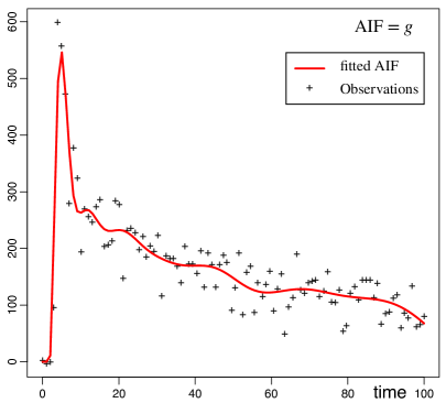
  Figure 2: Observations of an arterial input function (AIF) corresponding to kernel $g$ coming from one patient in the REMISCAN study [29] and fitted estimator of $g$ using an expansion over the system of the Laguerre functions with $M=17$.

• $g_{2}(t)=t^{2}e^{-0.1t}$ which aims to reproduce a long injection of contrast agent;

• $g_{3}(t)=t^{7}(100+t)^{-1}\,\exp\left(-0.9t^{3/4}\right)$ which describes an injection with a recirculation of the contrast agent inside the blood network.

Simulations were carried out for five different test functions $f$:

• $f_{1}(x)=\exp(-0.1x)$,

• $f_{2}(x)=\exp(-0.6x)$,

• $f_{3}(x)=0.5\,\exp(-0.1x)+0.5\,\exp(-0.6x)$,

• $f_{4}(x)=1-IG(2;0.5)$ where $IG(2;0.5)$ is the cdf of the gamma distribution with the shape parameter 2 and the scale parameter 0.5,

• $f_{5}(x)=(x+1)^{-1/3}$.

The value of $a$ in formula (2.1) was chosen so that to provide the best possible fit for the kernel $g$ when the number of terms in the expansion of $g$ is maximum, i.e. $m=M$.

The functions $f$ and $g$ are shown in Figure 3.

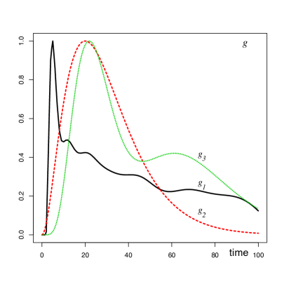
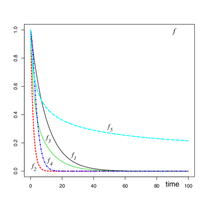
Figure 3: Test functions : (left) the kernel functions $g$ - (right) the estimated functions $f$

We illustrate performance of our methodology using kernel $g_{1}$ and test functions $f_{1}$, …, $f_{4}$. Figure 4 shows the observations and the true convolution for a medium signal-to-noise ratio 8. The associated estimators are presented in Figure 5. Here $SNR$ is defined as

$$SNR=\sqrt{\mbox{Var}(f)\big{/}(\sigma^{2}\ \mbox{Var}(g))}$$

where, for any function $\varphi$, we define $\mbox{Var}(\varphi)$ as

$$\mbox{Var}(\varphi)=\int_{0}^{T}\varphi^{2}(x)dx-\left[\int_{0}^{T}\varphi(x)dx\right]^{2}.$$

The idea of defining of $SNR$ in this manner is to remove the effect of convolution with $g$. This corresponds to SNR of Abramovich and Silverman (1998).

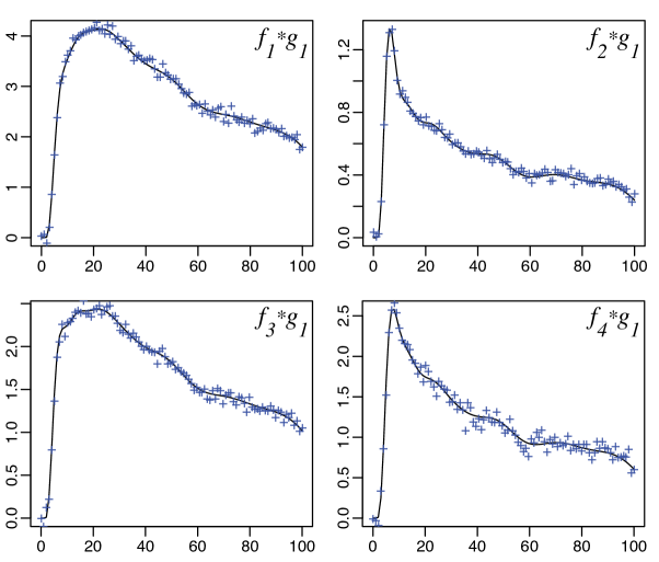
Figure 4: Observations and true convolutions of kernel $g_{1}$ with (unknown) functions $f_{1}$, …, $f_{4}$

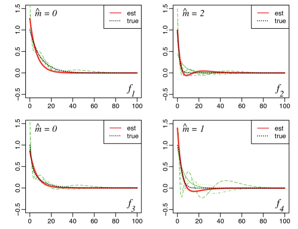
Figure 5: Estimators (thick plain line) and (unknown) functions (thick dotted line) $f_{1}$, …, $f_{4}$. Other fine dashed lines represent the estimates for $m=0,\ldots,5$. The selected value of $m$ is given by $\hat{m}$.

For simulations with $g_{1}(t)$ we chose $\beta=1$ in (1.1). We should mention that the value of $\beta$ is usually unknown in real-life situations. However, since in equation (1.1), $f(t)=\beta(1-F(t))$ where $F(t)$ is a cdf, one knows that $f(0)=\beta$ and, therefore, can estimate $\beta$ as $\hat{\beta}=\widehat{f(0)}$.

Table 1: The values of empirical risk increased by a factor of 100: $100\times\hat{R}(\hat{f})$. Empirical risks are computed for 400 samples for $g_{1}$, $g_{2}$ and $g_{3}$ and five functions of interest $f_{1}$, …, $f_{5}$.

$100\times\hat{R}(\hat{f})$		$n=100$					$n=200$
$SNR$		$f_{1}$	$f_{2}$	$f_{3}$	$f_{4}$	$f_{5}$	$f_{1}$	$f_{2}$	$f_{3}$	$f_{4}$	$f_{5}$
5	$g_{1}$	0.33	0.43	0.065	0.25	5.1	0.30	0.22	0.052	0.22	4.2
	$g_{2}$	0.27	0.37	0.063	0.25	5.1	0.22	0.15	0.051	0.16	4.0
	$g_{3}$	0.16	0.57	0.085	0.37	6.1	0.14	0.44	0.061	0.36	5.5
8	$g_{1}$	0.31	0.20	0.061	0.18	4.0	0.23	0.12	0.051	0.070	3.9
	$g_{2}$	0.23	0.18	0.062	0.11	4.0	0.06	0.14	0.050	0.031	3.6
	$g_{3}$	0.15	0.57	0.079	0.37	5.3	0.13	0.41	0.059	0.357	4.8
15	$g_{1}$	0.162	0.15	0.066	0.075	4.0	0.025	0.085	0.050	0.032	2.6
	$g_{2}$	0.022	0.17	0.061	0.037	3.4	0.012	0.115	0.050	0.027	2.8
	$g_{3}$	0.142	0.43	0.077	0.322	4.9	0.132	0.182	0.058	0.154	4.6

We executed simulations with $T=100$, $M=11$, two values of sample sizes, $n=100$ and $n=200$, and three signal-to-noise ratios (SNR), namely, $SNR=5,8$ and 15. The value 5 corresponds to real-life conditions, smaller values 8 and 15 correspond to noise level attained after the first denoising step as described in Rozenholc and Reiß (2012).

For a given trajectory, the empirical risk was evaluated as

$$\hat{r}(\hat{f})=n^{-1}\ \sum_{i=1}^{n}\left[\hat{f}(t_{i})-f(t_{i})\right]^{2}$$ (4.1)

and the average empirical risk, denoted $\hat{R}(\hat{f})$, is obtained by averaging the values of $\hat{r}(\hat{f})$ over 400 simulation runs. We used $B=1/2$ in penalty (2.16) and reduced the constant 4 in the penalty to 1.5 since this constant is an upper bound due to a triangular inequality. The value of $\alpha$ in (2.16) is chosen using condition (2.15) as follows. Since $2\log\rho_{m}\leq\log C_{\rho}+\alpha\log m$, $\alpha$ is selected by regressing $2\log\rho_{m}$ onto $\log m$ for $m=0,\ldots,6$.

Results of simulations are presented in Table 1. Table 1 verifies that indeed the methodology proposed in the paper works exceptionally well for functions $f_{i},i=1,\ldots,4$, and is still quite precise for test function $f_{5}$ for which Fourier transform does not even exist. The table demonstrates the effect of choosing parameter $a$: for function $f_{3}$ and $n=100$, the average empirical risk does not decline when SNR grows. This is due to the bias problem arising from the fact that $f_{3}$ is the sum of two exponentials and we fit only one value of $a$.

We also carried out a limited comparison of the method suggested above with the technique presented in Abramovich, Pensky and Rozenholc (2012). The comparison is performed using just one simple example where $f(x)=0.2\exp(-0.5x)+0.8\exp(-2x)$ and $g(t)=t^{2}(t+1)e^{-t}$ (see Figure 6). In this example, the value of $r$ in (3.1) is $r=3$ and we used $n=200$, $\sigma=0.025$ and $T=15$. It is easy to see from Figure 7 that the Laguerre functions based estimator outperforms the kernel estimator of Abramovich, Pensky and Rozenholc (2012) and also it does not exhibit boundary effects.

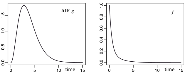
Figure 6: Functions $g$ (left) and $f$ (right) for comparison between deconvolution methods using adaptive kernels and penalized Laguerre functions.

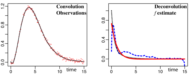
Figure 7: Comparison between deconvolution using kernel method and using penalized Laguerre functions : (left) $q=f*g$ and observations; (right) estimates $f$ : Penalized Laguerre deconvolution (thick plain line) - adaptive kernel estimation (thick dashed line) - true function $f$ (dotted line).

Finally, we compared our method to Singular Value Decomposition (SVD) techniques as described in the context of DCE imaging in Ostergaard et al. (1996) and Fieselmann et al. (2011). We tried various regularization methods including thresholding and Tikhonov regularization with rectangular or trapezoid rules for approximation of the convolution integral and played with the constant of regularization in order to find manually the best possible tuning in each case. In Figure 8 we display one of the best reconstructions which we managed to achieve with the SVD approach. One can clearly see how this technique fail to adequately recover unknown function $f$ : first, it introduces a shift, second, it produces estimators which fails to be a decreasing functions (recall that the function of interest in DCE imaging experiments is $f(t)=\beta(1-F(t))$ where $F(t)$ is a cdf and we use $\beta=1$ in our simulations). One reason for these shortcoming is that SVD estimates are smooth and degenerate at 0. As it is noted in the papers on DCE imaging (see, e.g., Fieselmann et al. (2011)), for convolution kernels corresponding to recirculation of the contrast agent (which is a common real-life scenario), SVD fails completely and needs some extra tuning in order to obtain quite poor results similar to those presented in Figure 8.

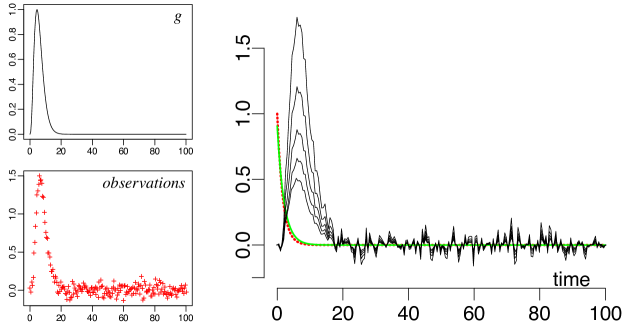
Figure 8: Comparison between deconvolution using SVD method with Tikhonov regularization and penalized Laguerre functions. SNR=8, $n=200$, $f=f_{1}$, (upper-left) the kernel $g(t)=t^{3}\exp(-t/3)$; (bottom-left) observations; (right) estimates $\hat{f}$ : Penalized Laguerre deconvolution (thick plain line) - SVD for various regularization constants (fine line) and true function $f$ (dotted line).

5 Discussion

In the present paper, we study a noisy version of a Laplace convolution equation. Equations of this type frequently occur in various kinds of DCE imaging experiments. We propose an estimation technique for the solutions of such equation based on expansion of the unknown solution, the kernel and the measured right-hand side over a system of the Laguerre functions. The number of the terms in the expansion of the estimator is controlled via complexity penalty. The technique leads to an estimator with the risk within a logarithmic factor of $m$ of the oracle risk under no assumptions on the model and within a constant factor of the oracle risk under mild assumptions.

The major advantage of the methodology presented above is that it is usable from a practical point of view. Indeed, the expansion results in a small system of linear equations with the matrix of the system being triangular and Toeplitz. The exact knowledge of the kernel is not required: the AIF curve can be fitted using data from DCE-CT experiments as it is shown in Figure 2. This distinguishes the present technique with the method of Abramovich, Pensky and Rozenholc (2012) (referenced later as APR) which strongly depends on the knowledge of the kernel in general and the value of $r$ in (3.1), in particular. After that, the method can be applied to any voxel of interest, either at the voxel level or using ROI (region of interest) manually drawn by a doctor or obtained using any clustering technique.

The method is computationally very easy and fast (requires solution of a small triangular system of linear equations) and produces no boundary effects due to extension at zero and cut-off at $T$. Moreover, application of the technique to discrete data does not require re-fitting the model for each model size separately. On the contrary, the vector of the Laguerre coefficients of the observed function is fitted only once, for the largest model size, and then is truncated for models of smaller sizes. The complexity of representation of $g$ adjusts to the complexity of representation of $f$ and the noise level. Moreover, if $g$ can be represented by a finite expansion over Laguerre functions with $k$ terms, the matrix of the system is $k$-diagonal.

The method performs very well in simulations. It is much more precise than the APR technique as Figure 7 confirms. In fact, the absence of exhaustive comparisons between the two methods is due to the fact that it is very tricky to produce estimators by the APR method, especially, in the case of $g_{1}$ which represents real life AIF. Similarly, as our study and Figure 8 show, the method is much more accurate than the SVD-based techniques.

There are few more advantages which are associated with the use of Laguerre functions basis. Since one important goal of future analysis of DCE-CT data is classification of the tissues and clustering of curves $f(t)=\beta(1-F(t))$ which characterize their blood flow properties, representation of the curves via Laguerre basis allows to replace the problem of classification of curves by classification of relatively low-dimensional vectors. In addition, due to the absence of boundary effects, the method allows to estimate classical medical parameters of interest $\beta$ which describes the perfusion of blood flow, and also $I_{f}=\int f(s)\,ds$ which characterizes the vascular mean transit time. These parameters can be estimated by $\hat{\beta}=1/\hat{f}(0)$ and $\hat{I}_{f}=\int\hat{f}(s)\,ds$, respectively.

The complexity of representation of $g$ is controlled by the choice of parameter $a$. Parameter $a$ is a non-asymptotic constant which does not affect the convergence rates. In practice, one can choose $a$ in order to minimize $\|g-\hat{g}_{M}\|$ where $\hat{g}_{M}$ is a fitted version of $g$ using the first $M$ Laguerre functions. Then, the same value of $a$ can be used in representation of the solution $f$. Our choice of $a$ provides a reasonable trade-off between the bias and the variance for majority of kernels considered above, including a real life AIF kernel coming from the REMISCAN (2007) study. However, our limited experimentation with choices of $a$ shows that there is room for improvement: undeniably, fine tuning parameter $a$ can improve estimation precision, especially, in the case when kernel $g$ has a strong exponential decay. However, this issue is a matter of future investigation.

6 Proofs

6.1 Proof of Theorem 1

Let $m,m^{\prime}\in{\mathcal{M}}_{n}$, $\mbox{\boldmath$t$}\in S_{m^{\prime}}$ and $\mbox{\boldmath$s$}\in S_{m}$. Denote $m^{*}=\max(m,m^{\prime})=m\vee m^{\prime}$, $\vec{\mbox{$\eta$}}_{m}=\sigma\sqrt{T/n}\ \vec{\mbox{$\xi$}}_{m}$ and observe that

$$\gamma_{n}(\mbox{\boldmath$t$})-\gamma_{n}(\mbox{\boldmath$s$}) = \|\mbox{\boldmath$t$}-\vec{\mbox{\boldmath$f$}}\|^{2}-\|\mbox{\boldmath$s$}-\vec{\mbox{\boldmath$f$}}\|^{2}-2\langle\mbox{\boldmath$t$}-\mbox{\boldmath$s$},\mbox{\boldmath$G$}_{M}^{-1}\vec{\mbox{$\eta$}}_{m^{*}}\rangle,$$ (6.1)

where $\vec{\mbox{\boldmath$f$}}=\vec{\mbox{\boldmath$f$}}_{M}$ is the vector of the true $M$ first coefficients of function $f$. Note that, due to orthonormality of the Laguerre system, for any $m$,

$$\|\hat{f}_{m}-f\|^{2}=\|\widehat{\vec{\mbox{\boldmath$f$}}}_{m}-\vec{\mbox{\boldmath$f$}}\|^{2}+\sum_{j=M}^{\infty}\left(f^{(j)}\right)^{2}\;\mbox{ and }\;\|f_{m}-f\|^{2}=\|\vec{\mbox{\boldmath$f$}}_{m}-\vec{\mbox{\boldmath$f$}}\|^{2}+\sum_{j=M}^{\infty}\left(f^{(j)}\right)^{2}.$$ (6.2)

Now, the definition of $\hat{m}$ yields that for any $m\in{\mathcal{M}}_{n}$ one has

$$\gamma_{n}(\widehat{\vec{\mbox{\boldmath$f$}}}_{\hat{m}})+\mbox{pen}(\hat{m})\leq\gamma_{n}(\vec{\mbox{\boldmath$f$}}_{m})+\mbox{pen}(m),$$

which with (6.1), implies

$$\|\widehat{\vec{\mbox{\boldmath$f$}}}_{m}-\vec{\mbox{\boldmath$f$}}\|^{2}\leq\|\vec{\mbox{\boldmath$f$}}_{m}-\vec{\mbox{\boldmath$f$}}\|^{2}+\mbox{pen}(m)+\Delta_{m,\hat{m}}.$$

Here $\Delta_{m,\hat{m}}=2\langle\hat{\vec{\mbox{\boldmath$f$}}}_{\widehat{m}}-\vec{\mbox{\boldmath$f$}}_{m},\mbox{\boldmath$G$}_{M}^{-1}\vec{\mbox{$\eta$}}_{m^{\star}}\rangle-\mbox{pen}(\widehat{m})$, where $m^{\star}=m\vee\widehat{m}$. Therefore, using (6.2), we obtain that, for any $m\in{\mathcal{M}}_{n}$,

$$\|\hat{f}_{\widehat{m}}-f\|^{2}\leq\|f_{m}-f\|^{2}+\mbox{pen}(m)+\Delta_{m,\hat{m}}$$ (6.3)

Note that, due to $2xy\leq(x^{2}/4)+4y^{2}$ for all $x>0,y>0$,

$$\Delta_{m,\hat{m}} \leq 2\|\hat{\vec{\mbox{\boldmath$f$}}}_{\widehat{m}}-\vec{\mbox{\boldmath$f$}}_{m}\|\sup_{\stackrel{{\scriptstyle\mbox{\boldmath$t$}\in S_{m^{\star}}}}{{\|\mbox{\boldmath$t$}\|=1}}}\langle\mbox{\boldmath$t$},\mbox{\boldmath$G$}_{M}^{-1}\vec{\mbox{$\eta$}}_{m^{\star}}\rangle-\mbox{pen}(\widehat{m})$$

$$\leq \frac{1}{4}\|\hat{\vec{\mbox{\boldmath$f$}}}_{\widehat{m}}-\vec{\mbox{\boldmath$f$}}_{m}\|^{2}+4\sup_{\stackrel{{\scriptstyle\mbox{\boldmath$t$}\in S_{m^{\star}}}}{{\|\mbox{\boldmath$t$}\|=1}}}\langle\mbox{\boldmath$t$},\mbox{\boldmath$G$}_{M}^{-1}\vec{\mbox{$\eta$}}_{m^{\star}}\rangle^{2}-\mbox{pen}(\widehat{m})$$

Now, denote

$$\tau(m,m^{\prime})=\frac{\sigma^{2}T}{n}\left[(1+B)v^{2}_{m^{*}}+2(1+B^{-1})(\alpha+1)\log(m^{*})\rho^{2}_{m^{*}}\right],$$ (6.4)

where $m^{*}=m\vee m^{\prime}$. Since, for any $m$, $\|\hat{\vec{\mbox{\boldmath$f$}}}_{\widehat{m}}-\vec{\mbox{\boldmath$f$}}_{m}\|^{2}\leq 2\|\hat{f}_{\widehat{m}}-f\|^{2}+2\|f_{m}-f\|^{2}$, then

$$\Delta_{m,\hat{m}} \leq \frac{1}{2}\,\|\hat{f}_{\widehat{m}}-f\|^{2}+\frac{1}{2}\,\|f_{m}-f\|^{2}+4\left[\sup_{\mbox{\boldmath$t$}\in S_{m\vee\widehat{m}}}\langle\mbox{\boldmath$t$},\mbox{\boldmath$G$}_{M}^{-1}\vec{\mbox{$\eta$}}_{m^{\star}}\rangle^{2}-\tau(m,\widehat{m})\right]_{+}$$

$$+ 4\tau(m,\widehat{m})-\mbox{pen}(\widehat{m}).$$

Using the fact that $4\tau(m,\widehat{m})\leq\mbox{pen}(m)+\mbox{pen}(\widehat{m})$, combining (6.3), (6.4) and (6.1), derive

$$\|\hat{f}_{\widehat{m}}-f\|^{2} \leq \|f_{m}-f\|^{2}+\mbox{pen}(m)+\frac{1}{2}\,\|\hat{f}_{\widehat{m}}-f\|^{2}+\frac{1}{2}\,\|f_{m}-f\|^{2}$$

$$+ 4\left[\sup_{\mbox{\boldmath$t$}\in S_{m\vee\widehat{m}}}\langle\mbox{\boldmath$t$},\mbox{\boldmath$G$}_{M}^{-1}\vec{\mbox{$\eta$}}_{m^{\star}}\rangle^{2}-\tau(m,\widehat{m})\right]_{+}.$$

Finally, subtracting $\,\|\hat{f}_{\widehat{m}}-f\|^{2}/2$ from both sides of the last equation and multiplying both sides by 2, obtain

$$\|\hat{f}_{\widehat{m}}-f\|^{2} \leq 3\|f_{m}-f\|^{2}+4\mbox{pen}(m)$$

$$+ 8\left[\sup_{\mbox{\boldmath$t$}\in S_{m\vee\widehat{m}}}\langle\mbox{\boldmath$t$},\mbox{\boldmath$G$}_{M}^{-1}\vec{\mbox{$\eta$}}_{m^{\star}}\rangle^{2}-\tau(m,\widehat{m})\right]_{+}.$$

Hence, validity of Theorem 1 rests on the following lemma which will be proved later.

Lemma 4.

Let condition (2.15) hold for some positive constants $\alpha$ and $C_{\rho}$. Then, for any $m$ and any $B>0$, one has

$${\mathbb{E}}\left[\sup_{\mbox{\boldmath$t$}\in S_{m\vee\widehat{m}},\|\mbox{\boldmath$t$}\|=1}\langle\mbox{\boldmath$t$},\mbox{\boldmath$G$}_{M}^{-1}\vec{\mbox{$\eta$}}_{m^{\star}}\rangle^{2}-\tau(m,\widehat{m})\right]_{+}\leq\frac{2C_{\rho}^{2}\sigma^{2}T}{mn}\left(1+\frac{1}{B}\right).$$

Proof of Lemma 4 is given in Section 6.3.

6.2 Proofs of Lemmas 2 and 3

Proof of Lemma 2. To prove this statement, we shall follow the theory of Wiener-Hopf integral equations described in Gohberg and Feldman (1974). Denote Fourier transform of a function $p(x)$ by $\hat{p}(\omega)=\displaystyle{\int_{-\infty}^{\infty}e^{i\omega x}p(x)dx}$ and observe that

$$\hat{\phi}_{k}(\omega)=(-1)^{k}\sqrt{2a}\frac{(a+i\omega)^{k}}{(a-i\omega)^{k+1}}.$$

Therefore, elements of the infinite Toeplitz matrix $G$ in (2.4) are generated by the sequence $b_{j}$, $j\geq 0$, where

$$b_{j} = (2a)^{-1/2}(g^{(j)}-g^{(j-1)})=\frac{1}{2\pi}\ \int_{-\infty}^{\infty}\hat{g}(\omega)\overline{[\hat{\phi}_{j}(\omega)-\hat{\phi}_{j-1}(\omega)]}d\omega$$ (6.7)

$$= \frac{a}{\pi}\int_{-\infty}^{\infty}\hat{g}(\omega)\left(\frac{i\omega-a}{i\omega+a}\right)^{j}\frac{d\omega}{a^{2}+\omega^{2}},\ \ j=0,1,\ldots.$$

Note that $|(i\omega-a)/(i\omega+a)|=1$, so that we can use the following substitution in the integral (6.7):

$$\frac{i\omega-a}{i\omega+a}=e^{-i\theta}\ \Longrightarrow\ \omega=\frac{a(e^{i\theta}+1)}{i(e^{i\theta}-1)}=\frac{a\sin\theta}{\cos\theta-1},\ \ 0\leq\theta\leq 2\pi.$$

Simple calculations show that

$$b_{j}=\frac{1}{2\pi}\ \int_{0}^{2\pi}\hat{g}\left(\frac{a(e^{i\theta}+1)}{i(+e^{i\theta}-1)}\right)e^{-i\theta j}d\theta,$$

so that $b_{j}$, $j\in{\mathbb{Z}}$, are Fourier coefficients of the function

$$B(\theta)=b(e^{i\theta})=\hat{g}\left(\frac{a(e^{i\theta}+1)}{i(e^{i\theta}-1)}\right).$$

Now, let us show that $b_{j}=0$ for $j<0$. Indeed, if $j=-k$, $k>0$, then

$$b_{j} = \frac{a}{\pi}\int_{-\infty}^{\infty}\hat{g}(\omega)\left(\frac{i\omega+a}{i\omega-a}\right)^{k}\frac{d\omega}{a^{2}+\omega^{2}}=\frac{a}{\pi}\int_{-\infty}^{\infty}\hat{g}(\omega)\left(\frac{i(-\omega)-a}{i(-\omega)+a}\right)^{k}\frac{d\omega}{a^{2}+\omega^{2}}$$

$$= \frac{1}{2\pi}\ \int_{-\infty}^{\infty}\hat{g}(\omega)\overline{[\hat{\phi}_{j}(-\omega)-\hat{\phi}_{j-1}(-\omega)]}d\omega=\int_{-\infty}^{\infty}g(x)\left[\phi_{k}(-x)-\phi_{k-1}(-x)\right]dx=0$$

since $g(x)=0$ if $x<0$ and $\phi_{k}(-x)=0$ if $x>0$. Hence, function $B(\theta)=b(e^{i\theta})$ has only coefficients $b_{j}$, $j\geq 0$, in its Fourier series. Now, to complete the proof, one just needs to note that $G(s)=\hat{g}(is)$ for any $s$ such that Laplace transform $G(s)$ of $g$ exists.

Proof of Lemma 3. Let us first find upper and lower bounds on $\|\mbox{\boldmath$G$}_{m}^{-1}\|_{2}^{2}=\mbox{Tr}(\mbox{\boldmath$G$}_{m}^{-T}\mbox{\boldmath$G$}_{m}^{-1})$ and $\|\mbox{\boldmath$G$}_{m}^{-1}\|^{2}=\lambda_{\max}(\mbox{\boldmath$G$}_{m}^{-T}\mbox{\boldmath$G$}_{m}^{-1})$. For this purpose, examine the function

$$b(z)=\hat{g}\left(\frac{a(z+1)}{i(z-1)}\right)=G\left(\frac{a(z+1)}{1-z}\right),\ \ |z|=1.$$

Denote $y=a(z+1)/(1-z)$, so that $z=(y-a)/(y+a)$ and $G(y)=b((y-a)/(y+a))$.

Let us show that, under Assumptions (A1)-(A4), $b(z)$ has a zero of order $r$ at $z=1$ and all other zeros of $b(z)$ lie outside the unit circle.

For this purpose, assume that $y=\alpha+i\beta$ is a zero of $G$, i.e. $G(\alpha+i\beta)=0$. Simple calculus yields

$$\left|\frac{y-a}{y+a}\right|^{2}=1-\frac{4\alpha a}{(\alpha+a)^{2}+\beta^{2}},$$

so that $|z|=|(y-a)/(y+a)|\leq 1$ iff $\alpha\geq 0$. But, by Assumption (A3), $G(y)$ has no zeros with nonnegative real parts, so that $\alpha<0$ and $|z|=|(y-a)/(y+a)|>1$. Therefore, all zeros of $b(z)$, which correspond to finite zeros of $G$, lie outside the complex unit circle ${\cal C}$.

Assumptions (A1), (A2) and properties of Laplace transform imply that $G(s)=s^{-r}(B_{r}+G_{r}(s))$ where $G_{r}(s)$ is the Laplace transform of $g^{(r)}(t)$. Hence,

$$\lim_{Re\ s\rightarrow\infty}s^{j}G(s)=\left\{\begin{array}[]{ll}0,&\mbox{if}\ \ j=0,...,r-1,\\ B_{r}\neq 0,&\mbox{if}\ \ j=r,\end{array}\right.$$

so that $y=\infty+i\beta$ is zero of order $r$ of $G(y)$. Since $\displaystyle{\lim_{Re\ y\rightarrow\infty}(y-a)/(y+a)=1}$, $b(z)$ has zero of order $r$ at $z=1$.

Then, $b(z)$ can be written as $b(z)=(1-z)^{r}w(z)$ where $w(z)$ is defined by formula (3.8) and all zeros of $w(z)$ lie outside the complex unit circle. Therefore, $w(z)$ can be written as

$$w(z)=C_{w}\prod_{j=1}^{N}(z-\zeta_{j}),\ \ 0\leq N\leq\infty,\ |\zeta_{j}|>1,$$ (6.8)

where $C_{w}$ is an absolute constant. Since $b(z)$ does not contain any negative powers of $z$ in its representation, $J_{0}=0$ and $J=0$ in (3.5) and, consequently, $\mbox{wind}(w)=0$. Also, by (3.4) and (3.8), one has $T^{-1}(b)=T(b^{-1})$ where $b^{-1}(z)=w^{-1}(z)(1-z)^{-r}$.

Now, recall that $\|\mbox{\boldmath$G$}_{m}^{-1}\|_{2}^{2}=\|T_{m}(b^{-1})\|_{2}^{2}$ and for $\|\mbox{\boldmath$G$}_{m}^{-1}\|^{2}=\|T_{m}(b^{-1})\|^{2}$. Using relation between Frobenius and spectral norms $\|\mbox{\boldmath$A$}_{1}\mbox{\boldmath$A$}_{2}\|_{2}\leq\|\mbox{\boldmath$A$}_{1}\|_{2}\|\mbox{\boldmath$A$}_{2}\|$ for any matrices $\mbox{\boldmath$A$}_{1}$ and $\mbox{\boldmath$A$}_{2}$ (see, e.g., Böttcher and Grudsky (2000), page 116), obtain

$$\|T_{m}(b^{-1})\|_{2}\leq\|T_{m}((1-z)^{-r})\|_{2}\|T_{m}(w^{-1})\|, \|T_{m}(b^{-1})\|\leq\|T_{m}((1-z)^{-r})\|\|T_{m}(w^{-1})\|,$$ (6.9)

$$\|T_{m}((1-z)^{-r})\|_{2}\leq\|T_{m}(b^{-1})\|_{2}\|T_{m}(w)\|, \|T_{m}((1-z)^{-r})\|\leq\|T_{m}(b^{-1})\|\|T_{m}(w)\|.$$ (6.10)

Note that (see Böttcher and Grudsky (2005), page 13)

$$\lim_{m\rightarrow\infty}\|T_{m}(w^{-1})\|=\|w^{-1}\|_{circ},\ \ \lim_{m\rightarrow\infty}\|T_{m}(w)\|=\|w\|_{circ},$$

Also, due to representation (6.8), both $w$ and $w^{-1}$ are bounded, and, therefore, $0<\|w^{-1}\|_{circ}<\infty$ and $0<\|w\|_{circ}<\infty$. Denote

$$\nu_{f}(m)=\|T_{m}((1-z)^{-r})\|_{2},\ \ \nu_{s}(m)=\|T_{m}((1-z)^{-r})\|.$$ (6.11)

Then, it follows from (3.6), (6.9) and (6.10) that, for $m$ large enough,

$$0.5\left(\|w\|_{circ}\right)^{-2}\ \nu_{f}^{2}(m) \leq \|T_{m}(b^{-1})\|_{2}^{2}\leq 2\|w^{-1}\|_{circ}^{2}\ \nu^{2}_{f}(m),$$ (6.12)

$$0.5\left(\|w\|_{circ}\right)^{-2}\ \nu_{s}^{2}(m) \leq \|T_{m}(b^{-1})\|^{2}\leq 2\|w^{-1}\|_{circ}^{2}\ \nu^{2}_{s}(m).$$ (6.13)

In order to finish the proof, we need to evaluate $\nu^{2}_{f}(m)$ and $\nu^{2}_{s}(m)$ and also to derive a relation between $v_{m}^{2}$, $\rho_{m}^{2}$, $\|T_{m}(b^{-1})\|_{2}^{2}$ and $\|T_{m}(b^{-1})\|^{2}$. The first task is accomplished by the following lemma.

Lemma 5.

Let $\nu_{f}(m)$ and $\nu_{s}(m)$ be defined in (6.11). Then,

$$2^{-(4r-1)}[(r-1)!]^{-2}m^{2r+1} \leq \nu^{2}_{f}(m)\leq 0.5m^{2r+1},$$ (6.14)

$$(r!)^{-2}m^{2r} \leq \nu^{2}_{s}(m)\leq m^{2r}.$$ (6.15)

Proof of Lemma 5 is given in Section 6.3.

Now, to complete the proof, recall that matrix $\mbox{$\Omega$}_{m}$ given by (2.8) is symmetric positive definite, so that there exist an orthogonal matrix $\mbox{\boldmath$U$}_{m}$ and a diagonal matrix $\mbox{\boldmath$D$}_{m}$, with eigenvalues of $\Omega$ as its diagonal elements, such that $\mbox{$\Omega$}_{m}=\mbox{\boldmath$U$}_{m}^{T}\mbox{\boldmath$D$}_{m}\mbox{\boldmath$U$}_{m}$ and $\mbox{$\Omega$}_{m}^{-1}=\mbox{\boldmath$U$}_{m}^{T}\mbox{\boldmath$D$}_{m}^{-1}\mbox{\boldmath$U$}_{m}$. Hence, by (2.10), (2.14) and Assumption (A4)

$$\|T_{m}(b^{-1})\|_{2}^{2} = \mbox{Tr}(\mbox{\boldmath$G$}_{m}^{-1}\mbox{\boldmath$G$}_{m}^{-T})=\mbox{Tr}(\mbox{\boldmath$G$}_{m}^{-1}\mbox{\boldmath$U$}_{m}^{T}\mbox{\boldmath$D$}_{m}\mbox{\boldmath$D$}_{m}^{-1}\mbox{\boldmath$U$}_{m}\mbox{\boldmath$G$}_{m}^{-T})$$

$$\leq \|\mbox{\boldmath$D$}_{m}^{-1}\|\|\sqrt{\mbox{\boldmath$D$}_{m}}\mbox{\boldmath$U$}_{m}\mbox{\boldmath$G$}_{m}^{-1}\|_{2}^{2}\leq\lambda_{1}^{-1}\mbox{Tr}(\mbox{\boldmath$G$}_{m}^{-T}\mbox{$\Omega$}_{m}\mbox{\boldmath$G$}_{m})=\lambda_{1}^{-1}v_{m}^{2},$$

$$v_{m}^{2} = \|\sqrt{\mbox{\boldmath$D$}_{m}}\mbox{\boldmath$U$}_{m}\mbox{\boldmath$G$}_{m}^{-1}\|_{2}^{2}\leq\lambda_{2}\|\mbox{\boldmath$G$}_{m}^{-1}\|_{2}^{2}=\lambda_{2}\|T_{m}(b^{-1})\|_{2}^{2},$$

$$\rho_{m}^{2} = \|\sqrt{\mbox{\boldmath$D$}_{m}}\mbox{\boldmath$U$}_{m}\mbox{\boldmath$G$}_{m}^{-1}\|^{2}\leq\lambda_{2}\|\mbox{\boldmath$G$}_{m}^{-1}\|^{2}=\lambda_{2}\|T_{m}(b^{-1})\|^{2},$$

so that

$$\rho_{m}^{2}\leq\lambda_{2}\|T_{m}(b^{-1})\|^{2},\ \ \lambda_{1}\|T_{m}(b^{-1})\|_{2}^{2}\leq v_{m}^{2}\leq\lambda_{2}\|T_{m}(b^{-1})\|_{2}^{2}.$$ (6.16)

Combination of (6.12) – (6.16) and Lemma 5 complete the proof.

6.3 Proofs of supplementary Lemmas

Proof of Lemma 4.

The proof of Lemma 4 has two steps. The first one is the application of a $\chi^{2}$-type deviation inequality stated in Laurent and Massart (2000), and improved by Gendre (see Lemma 3.10 of Gendre (2009)). The second step consists of integrating this deviation inequality.

The $\chi^{2}$-inequality is formulated as follows. Let $A$ be a $p\times p$ matrix $\mbox{\boldmath$A$}\in{\mathbb{M}}_{p}({\mathbb{R}})$ and $\zeta$ be a standard Gaussian vector. Denote $v_{A}^{2}=Tr(\mbox{\boldmath$A$}^{T}\;\mbox{\boldmath$A$})$ and $\rho^{2}(\mbox{\boldmath$A$})=\lambda_{{\rm max}}(\mbox{\boldmath$A$}^{T}\;\mbox{\boldmath$A$})$. Then, for any $x>0$,

$${\mathbb{P}}\left(\|\mbox{\boldmath$A$}\mbox{$\zeta$}\|^{2}\geq v_{A}^{2}+2\sqrt{v_{A}^{2}\rho^{2}(\mbox{\boldmath$A$})x}+\rho^{2}(\mbox{\boldmath$A$})x\right)\leq e^{-x}.$$ (6.17)

Now, recall that for $\mbox{\boldmath$t$}\in S_{m}+S_{m^{\prime}}=S_{m^{*}}$ where $m^{*}=m\vee m^{\prime}$, one has

$$\langle\mbox{\boldmath$t$},\mbox{\boldmath$G$}_{M}^{-1}\vec{\mbox{$\eta$}}_{m^{*}}\rangle\stackrel{{\scriptstyle\mathcal{L}}}{{=}}\frac{\sigma^{2}T}{n}\langle\mbox{\boldmath$t$}_{m^{*}},\sqrt{\mbox{\boldmath$Q$}_{m^{*}}}\mbox{$\zeta$}_{m^{*}}\rangle$$

where $\mbox{\boldmath$t$}_{m*}$ is the $m^{*}$-dimensional vector formed by the first $m^{*}$ coordinates of $t$ and $\mbox{$\zeta$}_{m^{*}}$ is a standard $m^{*}$-dimensional Gaussian vector. Moreover,

$$\sup_{\mbox{\boldmath$t$}\in S_{m}+S_{m^{\prime}},\|\mbox{\boldmath$t$}\|=1}\langle\mbox{\boldmath$t$},\mbox{\boldmath$G$}_{M}^{-1}\vec{\mbox{$\eta$}}_{m^{*}}\rangle^{2}=\|\sqrt{\mbox{\boldmath$Q$}_{m^{*}}}\mbox{$\zeta$}_{m^{*}}\|^{2}.$$

Thus, it follows from (6.17) that

$${\mathbb{P}}\left(\frac{n}{T\sigma^{2}}\|\sqrt{\mbox{\boldmath$Q$}_{m^{*}}}\mbox{$\zeta$}_{m^{*}}\|^{2}\geq v_{m^{*}}^{2}+2\sqrt{\rho_{m^{*}}^{2}v_{m^{*}}^{2}x}+\rho_{m^{*}}^{2}x\right)\leq e^{-x}.$$ (6.18)

For any $B>0$, one has $2\sqrt{\rho_{m^{*}}^{2}v_{m^{*}}^{2}x}\leq Bv_{m^{*}}^{2}+B^{-1}\rho_{m^{*}}^{2}x$ so that

$${\mathbb{P}}\left(\frac{n}{T\sigma^{2}}\|\sqrt{\mbox{\boldmath$Q$}_{m^{*}}}\mbox{$\zeta$}_{m^{*}}\|^{2}\geq(1+B)v_{m^{*}}^{2}+(1+B^{-1})\rho_{m^{*}}^{2}x\right)\leq e^{-x}.$$

Therefore, using definition (6.4) of $\tau(m,m^{\prime})$, obtain

$${\mathbb{E}}\left(\sup_{\mbox{\boldmath$t$}\in S_{m}+S_{m^{\prime}},\|\mbox{\boldmath$t$}\|=1}\langle\mbox{\boldmath$t$},\mbox{\boldmath$G$}_{M}^{-1}\vec{\mbox{$\eta$}}_{m^{*}}\rangle^{2}-\tau(m,m^{\prime})\right)_{+}={\mathbb{E}}\left(\|\sqrt{\mbox{\boldmath$Q$}_{m^{*}}}\mbox{$\zeta$}_{m^{*}}\|^{2}-\tau(m,m^{\prime})\right)_{+}$$

$$\leq \int_{0}^{+\infty}{\mathbb{P}}\left(\|\sqrt{\mbox{\boldmath$Q$}_{m^{*}}}\mbox{$\zeta$}_{m^{*}}\|^{2}-\frac{\sigma^{2}T}{n}\left[(1+B)v_{m^{*}}^{2}+2(1+B^{-1})(\alpha+1)\log(m^{*})\rho_{m^{*}}^{2}\right]\geq\xi\right)d\xi.$$

Changing variables

$$\frac{2\sigma^{2}T}{n}(\alpha+1)(1+B^{-1})\log(m^{*})\rho_{m^{*}}^{2}+\xi=\frac{\sigma^{2}T}{n}(1+B^{-1})\rho_{m^{*}}^{2}x$$

and application of (6.18) yield

$${\mathbb{E}}\left(\sup_{\mbox{\boldmath$t$}\in S_{m}+S_{m^{\prime}},\|\mbox{\boldmath$t$}\|=1}\langle\mbox{\boldmath$t$},\mbox{\boldmath$G$}_{M}^{-1}\vec{\mbox{$\eta$}}_{m^{*}}\rangle^{2}-\tau(m,m^{\prime})\right)_{+} \leq (1+B^{-1})\frac{\rho_{m^{*}}^{2}\sigma^{2}T}{n}\int_{2(\alpha+1)\log(m^{*})}^{+\infty}e^{-x}dx$$

$$= (1+B^{-1})\frac{\rho_{m^{*}}^{2}\sigma^{2}T}{n}(m^{*})^{-2(\alpha+1)}$$

$$\leq C_{\rho}(1+B^{-1})\frac{\sigma^{2}T}{n}(m^{*})^{-2}.$$

Recall that $m^{\star}=m\vee\hat{m}$ and obtain

$${\mathbb{E}}\left[\sup_{\mbox{\boldmath$t$}\in S_{m\vee\widehat{m}}}\langle\mbox{\boldmath$t$},\mbox{\boldmath$G$}_{M}^{-1}\vec{\mbox{$\eta$}}_{m^{\star}}\rangle^{2}-\tau(m,\widehat{m})\right]_{+}\leq\sum_{m^{\prime}\in{\mathcal{M}}_{n}}{\mathbb{E}}\left(\sup_{\mbox{\boldmath$t$}\in S_{m}+S_{m^{\prime}},\|\mbox{\boldmath$t$}\|=1}\langle\mbox{\boldmath$t$},\mbox{\boldmath$G$}_{M}^{-1}\vec{\mbox{$\eta$}}_{m\vee m^{\prime}}\rangle^{2}-\tau(m,m^{\prime})\right)_{+}$$

and

$$\sum_{m^{\prime}\in{\mathcal{M}}_{n}}{\mathbb{E}}\left(\sup_{\mbox{\boldmath$t$}\in S_{m}+S_{m^{\prime}},\|\mbox{\boldmath$t$}\|=1}\langle\mbox{\boldmath$t$},\mbox{\boldmath$G$}_{M}^{-1}\vec{\mbox{$\eta$}}_{m^{*}}\rangle^{2}-\tau(m,m^{\prime})\right)_{+}\leq C_{\rho}(1+B^{-1})\frac{\sigma^{2}T}{n}\sum_{m^{\prime}\in{\mathcal{M}}_{n}}(m\vee m^{\prime})^{-2}$$

$$\leq C_{\rho}(1+B^{-1})\frac{\sigma^{2}T}{n}\left(\sum_{m^{\prime}=1}^{m}m^{-2}+\sum_{m^{\prime}>m}(m^{\prime})^{-2}\right)$$

$$\leq C_{\rho}(1+B^{-1})\frac{\sigma^{2}T}{n}\left(m^{-1}+\int_{m}^{+\infty}\frac{dx}{x^{2}}\right)=2C_{\rho}(1+B^{-1})\frac{\sigma^{2}T}{nm},$$

which concludes the proof. $\Box$

Proof of Lemma 5. Note that, by formula 1.110 of Gradshtein and Ryzhik (1980),

$$(1-z)^{-r}=\sum_{j=0}^{\infty}{r+j-1\choose j}z^{j},$$

so that, by definition of Frobenius norm,

$$\|T_{m}((1-z)^{-r})\|^{2}_{2} = m^{2}+(m-1)^{2}{r\choose 1}^{2}+(m-2)^{2}{r+1\choose 2}^{2}+\ldots+{r+m-2\choose m-1}^{2}$$

$$= \sum_{j=0}^{m-1}{r+j-1\choose j}^{2}(m-j)^{2},$$

$$\|T_{m}((1-z)^{-r})\|^{2} = \max_{|z|=1}\left|\sum_{j=0}^{m-1}{r+j-1\choose j}z^{j}\right|=\sum_{j=0}^{m-1}{r+j-1\choose r-1}.$$

If $r=1$, then

$$\sum_{j=0}^{m-1}{r+j-1\choose j}^{2}(m-j)^{2}=\sum_{j=0}^{m-1}(m-j)^{2}=\frac{m(m+1)(2m+1)}{6}.$$

If $r\geq 2$, then

$$\frac{j^{r-1}}{(r-1)!}\leq{r+j-1\choose j}=\frac{(r-1+1)\ldots(r-1+j)}{(r-1)!}\leq(j+1)^{r-1},$$

so that, for $m\geq 4$,

$$\nu_{f}^{2}(m) = \|T_{m}((1-z)^{-r})\|^{2}_{2}\leq 0.5\,m^{2r+1},$$

$$\nu_{f}^{2}(m) \geq \sum_{j=m/4}^{3m/4}\frac{j^{2r-2}}{[(r-1)!]^{2}}(m-j)^{2}\geq\frac{m^{2r+1}2^{-(4r-1)}}{[(r-1)!]^{2}},$$

which proves validity of (6.14). To show that (6.15) holds, observe that, by formula 0.151.1 of Gradshtein and Ryzhik (1980),

$$\sum_{j=0}^{m-1}{r+j-1\choose r-1}={r+m-1\choose r},\ \ \frac{m^{r}}{r!}<{r+m-1\choose r}<m^{r}.$$

Fabienne Comte
Sorbonne Paris Cité
Université Paris Descartes,
MAP5, UMR CNRS 8145, France
fabienne.comte@parisdescartes.fr

Charles-André Cuenod
Sorbonne Paris Cité
Université Paris Descartes, PARCC
European Hospital George Pompidou (HEGP-APHP)
LRI, INSERM U970-PARCC, France
ca@cuenod.net

Marianna Pensky
Department of Mathematics
University of Central Florida
Orlando FL 32816-1353, USA
Marianna.Pensky@ucf.edu

Yves Rozenholc
Sorbonne Paris Cité
Université Paris Descartes,
MAP5, UMR CNRS 8145, France
yves.rozenholc@parisdescartes.fr

References

• [1] Abramovich, F., Pensky, M., Rozenholc, Y. (2012) Laplace deconvolution with noisy observations. ArXiv:1107.2766v2.
• [2] Abramovich, F., and Silverman, B.W. (1998). Wavelet decomposition approaches to statistical inverse problems. Biometrika, 85, 115-129.
• [3] Ameloot, M., Hendrickx, H. (1983) Extension of the performance of Laplace deconvolution in the analysis of fluorescence decay curves. Biophys. Journ., 44, 27 - 38.
• [4] Axel, L. (1980) Cerebral blood flow determination by rapid-sequence computed tomography: theoretical analysis. Radiology, 137, 679–686.
• [5] Böttcher, A., and Grudsky, S.M. (2000) Toeplitz Matrices, Asymptotic Linear Algebra, and Functional Analysis. Birkhauser Verlag, Basel-Boston-Berlin.
• [6] Böttcher, A., and Grudsky, S.M. (2005) Spectral Properties of Banded Toeplitz Matrices, SIAM, Philadelphia.
• [7] Carroll, R. J., and Hall, P. (1988). Optimal rates of convergence for deconvolving a density. J. Amer. Statist. Assoc. 83, 1184-1186.
• [8] Chauveau, D.E., van Rooij, A.C.M. and Ruymgaart, F.H. (1994). Regularized inversion of noisy Laplace transform. Adv. Applied Math. 15, 186–201.
• [9] Cinzori, A.C., and Lamm, P.K. (2000) Future polynomial regularization of ill-posed Volterra equations. SIAM J. Numer. Anal., 37, 949ñ979.
• [10] Comte, F., Rozenholc, Y., and Taupin, M.L. (2007) Finite sample penalization in adaptive density deconvolution. J. Stat. Comput. Simul., 77, 977–1000.
• [11] Delaigle, A., Hall, P. and Meister, A. (2008). On deconvolution with repeated measurements. Ann. Statist., 36, 665-685.
• [12] Dey, A.K., Martin, C.F. and Ruymgaart, F.H. (1998). Input recovery from noisy output data, using regularized inversion of Laplace transform. IEEE Trans. Inform. Theory, 44, 1125–1130.
• [13] Diggle, P. J., and Hall, P. (1993). A Fourier approach to nonparametric deconvolution of a density estimate. J. Roy. Statist. Soc. Ser. B, 55 523–531.
• [14] Fan, J. (1991). On the optimal rates of convergence for nonparametric deconvolution problem. Ann. Statist., 19, 1257-1272.
• [15] Fan, J. and Koo, J. (2002). Wavelet deconvolution. IEEE Trans. Inform. Theory, 48, 734–747.
• [16] Fieselmann, A., Kowarschik, M., Ganguly, A., Hornegger, J., and Fahrig, R. (2011) Deconvolution-based CT and MR brain perfusion measurement: theoretical model revisited and practical implementation details. Int. J. Biomed. Imaging, 2011, 467-563.
• [17] Gendre, X. (2009). Estimation par sélection de modèle en régression hétéroscédastique. PhD Thesis. http://tel.archives-ouvertes.fr/tel-00397608/fr/
• [18] Gripenberg, G., Londen, S.O., and Staffans, O. (1990) Volterra Integral and Functional Equations. Cambridge University Press, Cambridge.
• [19] Gohberg, I.C., Feldman, I.A. (1974) Convolution equations and projection methods for their solution. Amer. Math. Soc., Providence.
• [20] Gradshtein, I.S., Ryzhik, I.M. (1980) Tables of integrals, series, and products. Academic Press, New York.
• [21] Johnstone, I.M., Kerkyacharian, G., Picard, D. and Raimondo, M. (2004) Wavelet deconvolution in a periodic setting. J. Roy. Statist. Soc. Ser. B, 66, 547–573 (with discussion, 627–657).
• [22] Lamm, P. (1996) Approximation of ill-posed Volterra problems via predictor-corrector regularization methods. SIAM J. Appl. Math., 56, 524-541.
• [23] Laurent, B., Massart, P. B. (2000). Adaptive estimation of a quadratic functional by model selection. Ann. Statist., 28, 1302–1338.
• [24] Lien, T.N., Trong, D.D. and Dinh, A.P.N. (2008) Laguerre polynomials and the inverse Laplace transform using discrete data J. Math. Anal. Appl., 337, 1302–1314.
• [25] Maleknejad, K., Mollapourasl, R. and Alizadeh, M. (2007) Numerical solution of Volterra type integral equation of the first kind with wavelet basis. Appl. Math.Comput., 194, 400ñ405.
• [26] Ostergaard, L., Weisskoff, R.M., Chesler, D.A., Gyldensted, C., and Rosen, B.R. (1996) High resolution measurement of cerebral blood flow using intravascular tracer bolus passages. Part I: Mathematical approach and statistical analysis. Magn. Reson. Med., 36, 715–725.
• [27] Pensky, M., and Vidakovic, B. (1999). Adaptive wavelet estimator for nonparametric density deconvolution. Ann. Statist., 27, 2033–2053.
• [28] Polyanin, A.D., and Manzhirov, A.V. (1998) Handbook of Integral Equations, CRC Press, Boca Raton, Florida.
• [29] REMISCAN - Project number IDRCB 2007-A00518-45/P060407/STIC 2006; Research Ethics Board (REB) approved- cohort funding by INCa (1M Euros) and promoted by the AP-HP (Assistance Publique –Hôpitaux de Paris). Inclusion target: 100 patients. Ongoing since 2007.
• [30] Rozenholc, Y., and Reiß, M. (2012) Preserving time structures while denoising a dynamical image, Mathematical Methods for Signal and Image Analysis and Representation (Chapter 12), Florack, L. and Duits, R. and Jongbloed, G. and van Lieshout, M.-C. and Davies, L. Ed., Springer-Verlag, Berlin.
• [31] Stefanski, L., and Carroll, R. J. (1990). Deconvoluting kernel density estimators. Statistics, 21, 169-184.
• [32] Weeks, W.T. (1966) Numerical Inversion of Laplace Transforms Using Laguerre Functions. J. Assoc. Comput. Machinery, 13, 419 - 429.