Decay of Counterflow Quantum Turbulence in Superfluid ⁴He

Abstract

We have simulated the decay of thermal counterflow quantum turbulence from a statistically steady state at $T$=1.9[K], with the assumption that the normal fluid is at rest during the decay. The results are consistent with the predictions of the Vinen equation (in essence the vortex line density (VLD) decays as $t^{-1}$). For the statistically steady state, we determine the parameter $c_{2}$, which connects the curvature of the vortex lines and the mean separation of vortices. A formula connecting the parameter $\chi_{2}$ of the Vinen equation with $c_{2}$ is shown to agree with the results of the simulations. Disagreement with experiment is discussed.

PACS numbers: 67.25.dk,67.25.dg

1 Introduction

Superfluid ⁴He at a finite temperature behaves as an an intimate mixture of two components: an inviscid superfluid component (density $\rho_{{\mathrm{s}}}$ and velocity $\bm{v}_{\mathrm{s}}$); and a viscous normal component (density $\rho_{{\mathrm{n}}}$ and velocity $\bm{v}_{\mathrm{n}}$). Quantum turbulence^{1, 2} takes the form of a tangle of quantized vortices in the superfluid component; the normal fluid may or may not be turbulent. Thermal counterflow is an internal convection in which the superfluid component flows towards a source of heat, while the normal fluid, carrying all the entropy, flows away from it. There is a relative velocity $\bm{v}_{\mathrm{ns}}=\bm{v}_{\mathrm{n}}-\bm{v}_{\mathrm{s}}$ between the two fluids, with no net mass flow. When the counterflow velocity exceeds a certain critical value, laminar flow proves to be unstable and the superfluid component becomes turbulent. This was the first type of quantum turbulence to be identified experimentally in the late 1950s³.

The vortices in quantum turbulence interact with the normal fluid, giving rise a force of ”mutual friction” between the two fluids. The study of the characteristics of this mutual friction provided the experimental evidence for counterflow turbulence. The turbulence in the superfluid component can be characterized by the vortex line density (VLD), $L(t)$, and it was suggested that the time-evolution of this density in thermal counterflow might be described by the (Vinen) equation

$$\frac{dL}{dt}=\alpha\left|\bm{v}_{\mathrm{ns}}\right|L^{3/2}-\chi_{2}\frac{\kappa}{2\pi}L^{2},$$ (1)

where $\alpha$ and $\chi_{2}$ are temperature-dependent parameters and $\kappa$ is the quantum of circulation. The first term represents the generation of counterflow turbulence and the second term represents its decay. This equation implies that counterflow turbulence is homogeneous, which appears indeed to be the case as long as the spacing between vortices is much smaller than the size of the channel in which the heat current flows.

Since the 1950s, many experimental, theoretical and numerical studies of coun- terflow turbulence have been reported. Schwarz showed by numerical simulations with the vortex filament model⁴ that a self-sustained statistically steady-state form of turbulence can be maintained in the superfluid component⁵ by the mutual friction, and a more satisfactory simulation based on a full Biot-Savart simulation has recently been performed by Adachi et al.⁶. In both simulations flow of the normal fluid is assumed to be laminar. The steady-state turbulence is realized when the generation and decay terms in Eq. (1) balance, so that $L=L_{\mathrm{steady}}=\gamma^{2}v_{\mathrm{ns}}^{2}$, where $\gamma$ is a temperature-dependent parameter.

Counterflow turbulence in the steady state seems now to be well understood, but its decay, after the heat current is switched off, is less well understood. According to Eq.(1), with $v_{\mathrm{ns}}=0$, this decay should obey the equation

$$\frac{1}{L}=\chi_{2}\frac{\kappa}{2\pi}t+\frac{1}{L_{0}},$$ (2)

where $L_{0}$ is the initial VLD. However, it has been known for a long time that in practice the decay proceeds in a more complicated (non-monotonic) manner³, although there is some evidence that Eq. (2) is obeyed at small times. It seems now to be well established⁷ that for large times the decay proceeds as $t^{-3/2}$, implying that at this stage there is coupled motion of the two fluids dominated by eddies on a scale equal to the channel width⁸; i.e. the normal fluid is also turbulent.

In this paper we report the results of simulations of the decay of counterflow turbulence, starting from a statistically steady state, in order to check the predictions of Eq. (1). We assume that the normal fluid remains at rest during the decay. The validity of our simulations is limited to the extent that our VLDs are somewhat smaller than those encountered in practice, larger VLDs being hard to handle, but within this limitation our results prove to be consistent with the predictions of Eq. (1), with the expected value of $\chi_{2}$.

2 The simulation

We use the vortex filament model^{4, 5} and represent a vortex as a string of discrete points ${\bm{s}}\left(\xi,t\right)$, where $t$ is time and $\xi$ is arc length. At 0 K the velocity $\dot{\bm{s}_{0}}$ of the filament at the point ${\bm{s}}$ is given by

$$\dot{\bm{s}_{0}}=\frac{\kappa}{4\pi}{\bm{s}}^{\prime}\times{\bm{s}}^{\prime\prime}\ln\left(\frac{2\left(l_{+}l_{-}\right)^{1/2}}{e^{1/2}\xi_{0}}\right)+\frac{\kappa}{4\pi}\int_{\cal L}^{\prime}\frac{\left({\bm{s}}-{\bm{r}}\right)\times d{\bm{s}}}{\left|{\bm{s}}-{\bm{r}}\right|^{3}}+\bm{v}_{\mathrm{s}},$$ (3)

where the prime denotes differentiation with respect to arc length $\xi$, $l_{+}$ and $l_{-}$ are the lengths of the two adjacent line elements after discretization, separated by the point ${\bm{s}}$, and $\xi_{0}$ is the cutoff corresponding to the core radius. The first term shows the localized induction field arising from a curved line element acting on itself. The second term represents the non-local field obtained by carrying out the integral of the Biot-Savart law along the rest of the filament. The third term $\bm{v}_{s}$ is an applied field.

At finite temperatures, it is necessary to take into account of the mutual friction between the vortex core and the normal flow ${\bm{v}}_{{\mathrm{n}}}$, so that the velocity $\dot{\bm{s}}$ becomes

$$\dot{\bm{s}}=\dot{\bm{s}}_{0}+\alpha{\bm{s}}^{\prime}\times\left({\bm{v}}_{{\mathrm{n}}}-\dot{\bm{s}}_{0}\right)-\alpha^{\prime}{\bm{s}}^{\prime}\times\left[{\bm{s}}^{\prime}\times\left({\bm{v}}_{{\mathrm{n}}}-\dot{\bm{s}}_{0}\right)\right],$$ (4)

where $\alpha$ and $\alpha^{\prime}$ are temperature-dependent friction coefficients⁴, and $\dot{\bm{s}}_{0}$ is calculated from Eq. (3).

Some important quantities that are useful for characterizing the vortex tangle can introduced⁵. The VLD is

$$L=\frac{1}{\mathrm{\Omega}}\int_{\cal L}d\xi,$$ (5)

where the integral is performed along all vortices in the sample volume $\mathrm{\Omega}$. In the experiments^{3, 7}, the VLD was obtained from the attenuation of second sound propagating perpendicular to the counterflow $\bm{v}_{\mathrm{ns}}$. Because mutual friction acts only at right angles to a vortex line element, the directly measured quantity is not the real VLD given by Eq. (5), but rather a ”measured VLD”, given by

$$L_{p}=\frac{1}{\mathrm{\Omega}}\int_{\cal L}\mathrm{sin}^{2}\theta d\xi,$$ (6)

where $\theta$ is the angle between a vortex line segment and and the direction $\hat{\bm{r}}$ of propagation of the second sound. If the quantum turbulence is isotropic, $L_{p}=(2/3)L$. Anisotropy of the vortex tangle is also interesting and is described by the dimensionless parameters

$$I_{\parallel} = \frac{1}{\Omega L}\int_{\cal L}\left[1-\left(\bm{s}^{\prime}\cdot\hat{\bm{r}}_{\parallel}\right)^{2}\right]d\xi,$$ (7)

$$I_{\perp} = \frac{1}{\Omega L}\int_{\cal L}\left[1-\left(\bm{s}^{\prime}\cdot\hat{\bm{r}}_{\perp}\right)^{2}\right]d\xi,$$ (8)

where $\hat{\bm{r}}_{\parallel}$ and $\hat{\bm{r}}_{\perp}$ represent unit vectors parallel and perpendicular to the original heat flow (in our case $\hat{\bm{r}}_{\parallel}=\hat{\bm{z}}$). Since $\hat{\bm{r}}_{\perp}$ is the same as the direction of propagation of the second sound, then $L_{p}/L=I_{\perp}$. Symmetry generally yields the relation $I_{\parallel}/2+I_{\perp}=1$. If the vortex tangle is isotropic, the averages of these parameters are $\overline{I}_{\parallel}=\overline{I}_{\perp}=2/3$. At the other extreme, if the tangle consists entirely of curves lying in planes normal to $\bm{v}_{\mathrm{ns}}$, $\overline{I}_{\parallel}=1$ and $\overline{I}_{\perp}=1/2$.

In this study, calculations are performed under the following conditions. The numerical space resolution is $\Delta\xi=8.0\times 10^{-4}$[cm], the time resolution is $\Delta t=1.0\times 10^{-4}$[s], temperature is 1.9[K], and the computing box size is $0.1\times 0.1\times 0.1$[cm³]. We use periodic conditions in all directions.

3 Results

3.1 Turbulence in the statistically steady state

Our decays start from a statistically steady state, and it is instructive first to describe the character of this state and how it is generated⁶.

First, we place in the box six vortex rings moving towards its centre, and we impose the relative velocity, $v_{\mathrm{ns}}=0.52$[cm/s], along the $z$-axis at $T$=1.9[K]. The vortices make many reconnections and the VLD increases until it becomes statistically steady. The VLD of this steady state turbulence is $L_{0}\sim 6.04\times 10^{3}[1/\mathrm{cm}^{2}]$ and it satisfies the equation $L=\gamma^{2}v_{\mathrm{ns}}^{2}$.

We investigated the relationship⁵ between the curvature of the vortex lines and the mean distance between vortices, $l=1/L^{1/2}$,

$$\left<\frac{1}{R^{2}}\right>=c_{2}^{2}\frac{1}{l^{2}},$$ (9)

where the left hand side is the mean square curvature of the vortex lines and $c_{2}$ is a temperature-dependent parameter. The parameter $c_{2}$ tends to decrease with increasing temperature, because the high velocities associated with small radii of curvature are more strongly damped by mutual friction at high temperature.

(a)

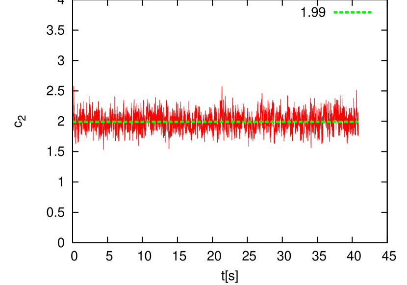
(b)

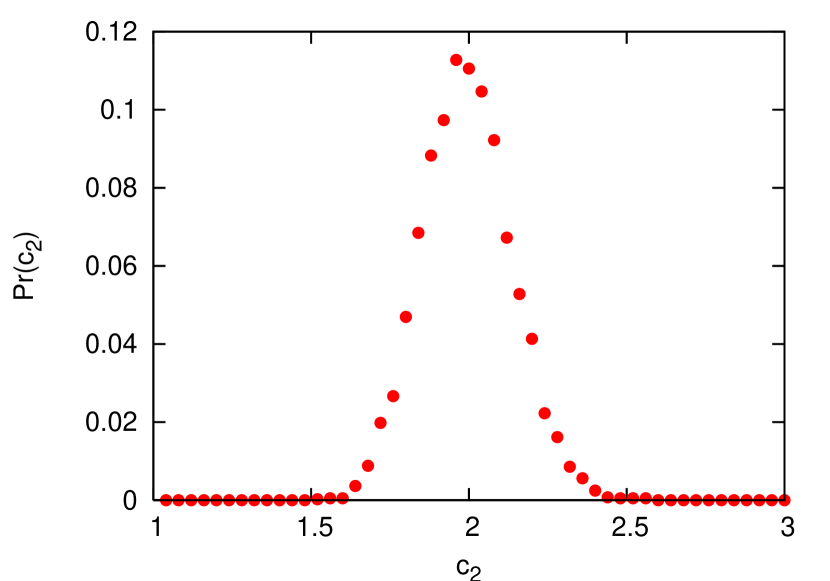
Figure 1: (Color online) (a) Dependence of $c_{2}$ on time in the statistically steady state. The parameter $c_{2}$ fluctuates around 1.99. (b) Distribution of $c_{2}$. The peak value is $c_{2}=1.96$ and the standard deviation is $\sigma_{c_{2}}=0.38$.

Figure 1 (a) shows that the parameter $c_{2}$ is statistically constant and the time average of $c_{2}$ is 1.99. Apparently, the fluctuation of $c_{2}$ comes from the fluctuations in the statistically steady state of the VLD and the mean square curvature. We plot the probability density distribution of $c_{2}$ in Fig. 1 (b) obtaining $c_{2}=1.99\pm 0.38$, where the error is a standard deviation. The dependence of $c_{2}$ on temperature will be reported in another paper.

3.2 Decay of the counterflow turbulence

After we obtained the steady state, we turned off the relative velocity, so that the turbulence can decay. It is necessary to study the statistics of the decaying turbulence, because the relatively small initial VLDs lead to fluctuations of the decaying VLD that are not negligible in one decay. Therefore we simulated 41 decays from slightly different initial conditions, and then averaged the results. Figure 3 shows these averaged results, in the form of plots of $L$ and $1/L$ against time. Red circle points are the real VLDs and green triangle points show how the ”measured VLDs” are expected to behave.

Figure 2 shows the configuration of vortices in the decaying turbulence at various times. As we demonstrate below, the configuration is initially anisotropic (a), but after about 0.5[s] it becomes isotropic (b), until at times greater than about 3[s] the line density becomes so small (line spacing comparable with the size of the box) that the decay is strongly influenced by the walls of the box.

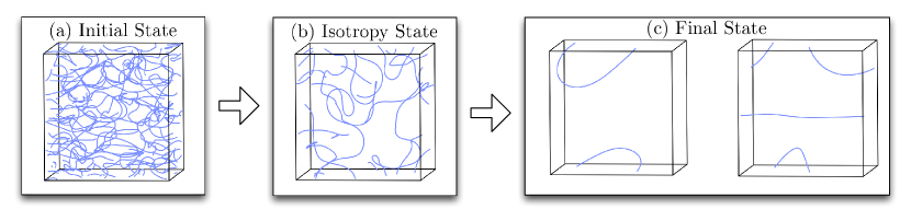
Figure 2: (Color online) Configuration of the vortex tangle at (a) $t$=0.0[s], (b) $t\sim$0.5[s], and (c) $t>$3.0[s].

We see from Fig. 3 that an equation of the form of Eq. (2) is obeyed as long as the VLD is not so small that the decay is influenced by the walls of the box. This result applies to both the real VLD and the measured VLD.

It was argued in reference⁹ from a consideration of the total rate of energy dissipation due to mutual friction that $\chi_{2}$ and $c_{2}$ can be expected to be related by the equation

$$\chi_{2}=\frac{\alpha c_{2}^{2}}{2}\ln{\frac{R_{0}}{\xi_{0}}},$$ (10)

where $R_{0}=1/(L_{0}c_{2}^{2})$ and $L_{0}$ is an initial VLD. In this way we can predict that at 1.9[K] $\chi_{2}=5.48\pm 0.88$. We see from Fig. 3 that our simulations support this prediction.

(a) @

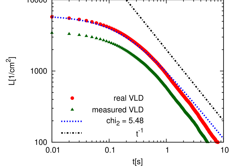
(b)

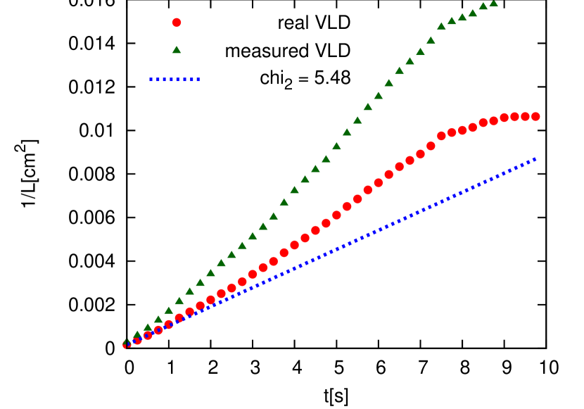
Figure 3: (Color online) The decay of VLD (red circle points) and the measured VLD (green triangle points). These figures are averaged data. Figure (a) is a log-log plot of $L$ against $t$, and Fig. (b) is a normal plot of $1/L$ against $t$. The blue dotted line is the solution of Vinen equation ($\chi_{2}=5.48$). The black dot-dashed line shows $t^{-1}$ power law.

The way in which the degree of anisotropy changes during the decay is shown in Fig. 4, in which we have plotted the ratio $L_{p}/L$ and the parameter $I_{\parallel}$ against time. For isotropic turbulence $L_{p}/L=I_{\parallel}=2/3$.

(a)

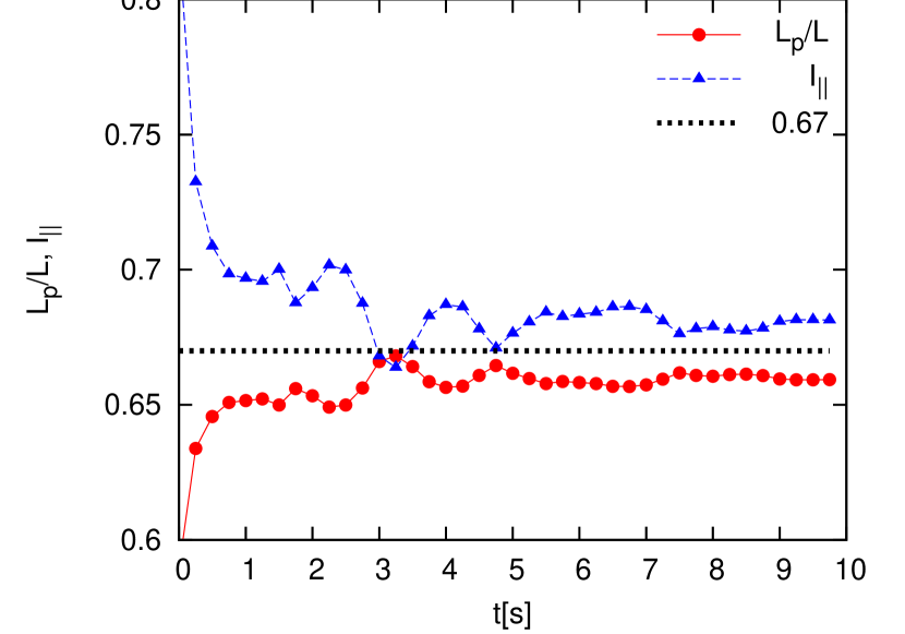
(b)

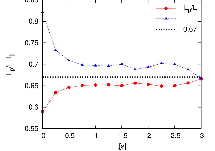
Figure 4: (Color online) The ratio of $L_{p}$ to $L$ (red circle points) and the anisotropy parameter, $I_{\parallel}$, (blue triangle points), plotted against time. The black dotted lines shows 2/3.

As we have ready noted, the decay at times greater than $\sim$3[s] is strongly influenced by the walls of the box, and this can be seen in the behavior of $L_{p}/L$ in Fig. 4 (a). Figure 4 (b) shows that the decaying turbulence remains strongly anisotropic until $t\sim$0.5[s]. In the interval between $t$=0.5[s] and $t$=2.5[s], the averages of $L_{p}/L$ and $I_{\parallel}$ are $0.65\pm 0.04$ and $0.70\pm 0.08$, both values being close to 2/3, indicating that the turbulence has become approximately isotopic.

4 Conclusions

We have carried out computer simulations of the decay of quantum turbulence, using the vortex filament model^{4, 5}, with the assumption that the normal fluid is stationary during the decay. The simulations start from a statistically steady state of thermal counterflow turbulence⁶ (Fig. 2 (a)), generated by a flow in which $v_{\mathrm{s}}-v_{\mathrm{n}}=0.52$[cm/s] at a temperature of 1.9[K]. The results prove to be consistent with the predictions of the Vinen equation (essentially the vortex line density decays with time as $t^{-1}$ in the limit of large times, as long as the line spacing is small compared with the box size). A parameter $c_{2}$, which describes the relationship between the curvature of the vortex lines and the mean distance between vortices, was evaluated for the steady state, and it is shown that the value of a parameter $\chi_{2}$ that appears in the Vinen equation is correctly predicted in terms of $c_{2}$ by a formula derived by Vinen and Niemela⁹. The turbulence is markedly anisotropic in the steady state counterflow, but it becomes isotropic as the decay proceeds. The validity of these results at temperatures other than 1.9[K] will be investigated in future work.

The type of decay that emerges from our simulations does not agree with experiment, as has been suspected for many years. The origin of the discrepancy has been discussed by Schwarz and Rozen¹⁰ and by Barenghi et al.¹¹. Our results do not add support to the idea of Barenghi et al. that the discrepancy is associated in part with the transition during decay from an anisotropic to an isotropic vortex configuration. We suspect that the discrepancy is due primarily to the existence of coupled motion of the two fluids during the decay (perhaps even in the steady state), as suggested by Schwarz and Rozen.