A generalized fluctuation relation for power-law distributions

Abstract

Strong violations of existing fluctuation theorems may arise in nonequilibrium steady states characterized by distributions with power-law tails. The ratio of the probabilities of positive and negative fluctuations of equal magnitude behaves in an anomalous nonmonotonic way [H. Touchette and E.G.D. Cohen, Phys. Rev. E 76, 020101(R) (2007)]. Here, we propose an alternative definition of fluctuation relation (FR) symmetry that, in the power-law regime, is characterized by a monotonic linear behavior. The proposal is consistent with a large deviation-like principle. As example, it is studied the fluctuations of the work done on a dragged particle immersed in a complex environment able to induce power-law tails. When the environment is characterized by spatiotemporal temperature fluctuations, distributions arising in nonextensive statistical mechanics define the work statistics. In that situation, we find that the FR symmetry is solely defined by the average bath temperature. The case of a dragged particle subjected to a Lévy noise is also analyzed in detail.

I Introduction

Fluctuation theorems have become a standard tool to characterize nonequilibrium states gallavoti ; Jarzynski ; kurchan ; spohn ; crocks ; maes ; seifert . Independently of their specific formulation searles ; vulpiani ; mukamel ; JarzynskiReport , a common underlying ingredient is an assertion about the symmetries of the fluctuations measures. For example, one of the most common formulation establishes that the probability of positive and negative fluctuations of a given variable differ by an exponential weight proportional to the fluctuations magnitude. This FR symmetry has been confirmed in a wide class of experimental setups PRLexper . While most of the analysis focus on variables such as entropy production and work (performed on a system), the FR symmetries may also be valid for nonthermodynamic variables soodPituto .

A Brownian particle dragged by a spring through a thermal environment is one of the simpler arrangement where a FR symmetry can be theoretically predicted mazonka ; zon and measured wangBrownianExp . While the work performed on the particle satisfy a standard or conventional FR, the heat fluctuations follow and extended FR FTExtended . The exponential weight that relates the probability of positive and negative fluctuations does not scale linearly with the heat variable. Similar deviations with respect to a linear dependence have been found in the injected power to systems driven by an external stochastic force cohenPoisson ; FTNonLinear .

Conventional or extended FRs FTExtended ; cohenPoisson ; FTNonLinear are essentially valid when the probability distributions obey a large deviation principle (LDP) touchette ; sornette . This formalism also provides a solid basis for characterizing nonequilibrium states garrahan . Therefore, stronger violations of conventional FRs should arise when power-law distributions sornette determine the fluctuations statistics. In fact, self-similar structures can not be studied in the context of a standard large deviation theory sornette ; touchette .

One of the first analysis about the incompatibility of FRs with anomalous (power-law distributed) fluctuations was done by Touchette and Cohen in Ref. cohenRapid . In contrast with previous Langevin models mazonka ; zon , where the environment influence is taken into account through a Gaussian white noise, they considered a stable Lévy white noise. It was found that the ratio of the probabilities of positive and negative work fluctuations of equal magnitude behaves in an anomalous nonlinear way, developing a convergence to one for large fluctuations. Hence, negative fluctuations of the work performed on the particle are just as likely to happen as large positive work fluctuations of equal magnitude. This non-usual property strongly departs from the Gaussian case, where the validity of a standard FR implies that positive fluctuations are exponentially more probable than negative ones.

A similar analysis on anomalous fluctuation properties was performed by Chechkin and Klages klages for the same kind of Langevin models. In the (power-law) Lévy case the same conclusions were obtained. On the other hand, it was shown that standard FRs remain valid in presence of normal long time correlated fluctuations. The long-range correlations only alter the time-speed of the large deviation functions (LDFs) touchette . An analogous conclusion was obtained by Harris and Touchette harris .

In Ref. BeckCohenFT Beck and Cohen introduced an alternative FR that arises by considering a superstatistical model beckQ ; superstatistics , where the particle environment develops (spaciotemporal) temperature fluctuations. As is well known beckQ , this dynamics leads to power-law distributions arising in Tsallis nonextensive statistical mechanics TsallisBook ; Qlectures ; qConstraints ; stepestQ ; QCentralLimit ; LevyAsQ ; QFokker . The alternative FR was derived by averaging temperature in a standard FR. When the “measured” work distribution develops power-law tails BeckCohenFT , a very complex expression that does not has a clear physical meaning is obtained.

From different points of view, all quoted analysis klages ; BeckCohenFT sustain the main conclusion of Ref. cohenRapid , that is, FRs in presence of power-law distributions acquire an anomalous (complicated) structure whose origin can be linked to the incompatibility of self-similar structures with a (standard) LDP. The main goal of this paper is to introduce a generalized and alternative FR such that in presence of power-law tails the symmetry between positive and negative fluctuations is expressed through a linear dependence. Hence, a simple scheme for understanding previous results cohenRapid ; klages ; harris ; BeckCohenFT is obtained. Furthermore, we associate the proposed symmetry with a large deviation-like principle. In a long time regime, it allows expressing the FR through the symmetries of a set of LDFs associated to the probability distribution and its characteristic function. As in the standard case spohn , both functions are related by a Legendre-Fenchel transformation touchette .

Similarly to the case of standard FR, the proposed probability symmetry does not assume an underlying thermodynamic equilibrium, either extensive or nonextensive. Nevertheless, the alternative FR symmetry adopts a very simple structure when written in terms of a set of functions introduced in nonextensive entropy formalism TsallisBook ; Qlectures . The relevance of this stretched relation becomes evident when considering previous related analysis BeckCohenFT . Furthermore, it is expected that a FR associated to a nonextensive (stochastic) thermodynamics may have a central role for understanding intrinsic fluctuations in nanoscale systems NanoSuperFT .

The paper is outlined as follows. In Sec. II we introduce the generalized FR symmetry. In Sec. III we apply the alternative definition to a specific physical system characterized by power-law tails. It is analyzed the fluctuations of the work done on a dragged particle immersed in a complex environment that develops (spatiotemporal) temperature fluctuations BeckCohenFT . Furthermore, the Lévy model introduced in Ref. cohenRapid is analyzed in detail. In Sec. IV we give the conclusions. In Appendix A we develop a large deviation-like principle and characterize the symmetries of the LDFs. These last results rely on a saddle-point approximation performed in Appendix B.

II Generalized fluctuation relation

For an arbitrary stochastic variable $x_{st},$ with probability distribution $p(x),$ a standard FR symmetry is defined by the relation $\ln[p(x)/p(-x)]=\zeta x,$ or equivalently $p(\pm x)=p(\mp x)e^{\pm\zeta x},$ where $\zeta$ is a positive constant. Here, we propose the alternative FR symmetry

$$\frac{[p(x)]^{1-q}-[p(-x)]^{1-q}}{1-q}=\zeta x,$$ (1)

which in turn can be expressed as

$$p(\pm x)=\{[p(\mp x)]^{1-q}\pm(1-q)\zeta x\}^{\frac{1}{1-q}}.$$ (2)

The real parameter $q$ is related with the index of the power-law tails. Its domain will be specified later on. The units of the constant $\zeta$ are $[1/x]^{2-q}.$ Nevertheless, in the standard case it is a conjugate variable of $x,$ that is, its units are $[1/x].$ This discrepancy can be avoided by writing

$$\zeta=\frac{\zeta_{ph}}{\int_{-\infty}^{\infty}dx[p(x)]^{q}},$$ (3)

where now $\zeta_{ph}$ play the role of a (physical) conjugate variable. Notice that even with this parameter redefinition, the proposed symmetry can be written solely in terms of $p(x).$ The generalized FR written in terms of $\zeta$ is called “unnormalized scheme,” while in terms of $\zeta_{ph}$ “normalized scheme.”

The previous relations, Eqs. (1) and (2), strongly departs from the standard ones. Their structure is simplified by writing them in terms of a set of functions introduced previously in the context of Tsallis nonextensive statistical mechanics TsallisBook . A q-logarithm and q-exponential functions are defined respectively as

$$\ln_{q}x\equiv\frac{x^{1-q}-1}{1-q},\ \ \ \ \ e_{q}^{x}\equiv[1+(1-q)x]^{\frac{1}{1-q}},$$ (4)

jointly with the generalized q-product operation

$$x\otimes_{q}y\equiv[x^{1-q}+y^{1-q}-1]^{\frac{1}{1-q}}.$$ (5)

The relevance of these definitions comes from the property that in the limit $q\rightarrow 1$ they recover the standard logarithm $[\ln_{1}x=\ln x],$ the exponential function $[\exp_{1}x=\exp x],$ and respectively the standard product $[x\otimes_{1}y=xy].$ In terms of them, Eq. (1) can be written as

$$\ln_{q}[p(x)]-\ln_{q}[p(-x)]=\zeta x,$$ (6)

while Eq. (2) becomes equivalent to

$$p(-x)=p(x)\otimes_{q}e_{q}^{-\zeta x},\ \ \ \ \ \ p(x)=p(-x)\otimes_{q}e_{q}^{\zeta x}.$$ (7)

Hence, the proposed FR can be read as a “deformation” of the standard ones. The parameter $q$ measures the degree of departure with respect to the standard case $(q\rightarrow 1).$ Notice that by using the properties $\ln_{q}(x\otimes_{q}y)=\ln_{q}x+\ln_{q}y,$ and $e_{q}^{x+y}=e_{q}^{x}\otimes_{q}e_{q}^{y}$ TsallisBook , the consistence between the previous two expressions becomes evident.

The standard FR symmetry can also be written in terms of the characteristic function $Z(\lambda)=\int_{-\infty}^{\infty}dxp(x)e^{-\lambda x},$ that is, $Z(\lambda)=Z(-\lambda+\zeta),$ which in turn implies $Z(\zeta)=1.$ Taking into account Eq. (2), it follows that here we must consider the generalized expression

$$Z_{q}(\lambda)\equiv\int_{-\infty}^{\infty}dx\{[p(x)]^{1-q}-(1-q)\lambda x\}^{\frac{1}{1-q}},$$ (8)

which can be rewritten as

$$Z_{q}(\lambda)=\int_{-\infty}^{\infty}dx[p(x)\otimes_{q}e_{q}^{-\lambda x}].$$ (9)

By using the associative property $x\otimes_{q}(y\otimes_{q}z)=(x\otimes_{q}y)\otimes_{q}z$ TsallisBook , the generalized FR [Eq. (6) or (7)] implies the equivalent symmetry

$$Z_{q}(\lambda)=Z_{q}(-\lambda+\zeta),\ \ \ \ \ \ \ \ \ \ \ \ \ \ Z_{q}(\zeta)=1.$$ (10)

Notice that this condition is exactly the same that defines the standard case, $q\rightarrow 1.$

The expression (9) naturally arises in nonextensive statistical mechanics. Hence, it properties are well known TsallisBook . $Z_{q}(\lambda)$ is the generating function of a kind of generalized moments of $x_{st},$ which are calculated from powers of $p(x).$

In accordance with the normalized scheme [Eq. (3)], we introduce the definitions

$$Z_{q}^{ph}(\lambda_{ph})\equiv Z_{q}(\lambda(\lambda_{ph})),\ \ \ \ \ \ \ \ \ \lambda=\frac{\lambda_{ph}}{\int_{-\infty}^{\infty}dx[p(x)]^{q}}.$$ (11)

Thus, Eqs. (3) and (10) allows us to write the equivalent symmetry

$$Z_{q}^{ph}(\lambda_{ph})=Z_{q}^{ph}(-\lambda_{ph}+\zeta_{ph}),\ \ \ \ \ \ \ \ \ \ \ \ \ \ Z_{q}^{ph}(\zeta_{ph})=1.$$ (12)

II.1 q-Gaussian distributions

The relations (6) and (7) define the generalized FR. Equivalently, it can be expressed through the “q-characteristic function” (9) leading to Eq. (10). Here, we search which kind of distributions may satisfy these relations in an exact way for any value of $x.$

Gaussian distributions always satisfy the standard symmetry corresponding to $\lim q\rightarrow 1.$ Normal distributions emerge naturally when formulating a central limit theorem, as solutions of linear Fokker-Planck equations, or by maximizing Gibbs entropy under a second moment constraint. Similarly, q-Gaussian distributions TsallisBook are related to a generalized central limit theorem QCentralLimit , are solutions of a kind of non-linear Fokker-Planck equations QFokker , and maximize nonextensive Tsallis entropy under a generalized second moment constraint qConstraints . They read

$$p(x)=\frac{\sqrt{\beta}}{\mathcal{N}_{q}}\exp_{q}[-\beta(x-x_{0})^{2}],$$ (13)

where $\beta^{-1}$ measures the width of the distribution and $\mathcal{N}_{q}$ is a normalization factor such that $\int_{-\infty}^{+\infty}p(x)dx=1,$ $(q<3).$ For $1<q<3,$ $p(x)$ is characterized by power-law tails, $p(x)\simeq 1/(x-x_{0})^{2/(q-1)},$ which is the case of interest in this paper. Hence, the index $q$ determines the exponent of the power-law tails. The first moment of $p(x)$ is finite for $1<q<2,$ while the second one for $1<q<5/3.$ In the domain $1<q<3,$ the normalization constant reads TsallisBook

$$\mathcal{N}_{q}=\sqrt{\frac{\pi}{q-1}}\ \frac{\Gamma(\frac{3-q}{2(q-1)})}{\Gamma(\frac{1}{q-1})},\ \ \ \ \ \ 1<q<3,$$ (14)

where $\Gamma(y)$ is the Gamma function.

It is immediate to prove that the generalized FR (6) [or Eq. (7)] is satisfied, for any value of $x,$ by the q-Gaussian distribution (13) with

$$\zeta=4x_{0}\frac{\beta^{\frac{3-q}{2}}}{\mathcal{N}_{q}^{1-q}},\ \ \ \ \ \ \ \ \ \ \ \zeta_{ph}=4x_{0}\beta\Big{(}\frac{3-q}{2}\Big{)}.$$ (15)

In the second expression we used the integral

$$\int_{-\infty}^{+\infty}[p(x)]^{q}dx=\Big{(}\frac{3-q}{2}\Big{)}\Big{(}\frac{\mathcal{N}_{q}}{\sqrt{\beta}}\Big{)}^{1-q},$$ (16)

valid for the distribution (13). When $q\rightarrow 1,$ it follows the standard Gaussian expression $\zeta=\zeta_{ph}=4x_{0}\beta.$ On the other hand, it is simple to realize that an arbitrary distribution $p(x)$ satisfy the symmetry (6) when $x$ is restricted to the interval where it develops power-law tails, $p(x)\simeq 1/(x-x_{0})^{2/(q-1)}.$ Hence, even in presence of power-law tails, a linear relation characterize the symmetry between positive and negative fluctuations of equal magnitude.

Using that $\int_{-\infty}^{+\infty}\exp_{q}(-ax^{2})=\mathcal{N}_{q}/\sqrt{a},$ after some algebra the q-characteristic function (9) associated to the q-Gaussian distribution (13) reads

$$Z_{q}(\lambda)=\exp_{\tilde{q}}\Big{\{}\!\Big{(}\frac{3-q}{2}\Big{)}\!\Big{(}\frac{\mathcal{N}_{q}}{\sqrt{\beta}}\Big{)}^{1-q}\Big{[}\frac{\lambda^{2}\mathcal{N}_{q}^{1-q}}{4\beta^{\frac{3-q}{2}}}-\lambda x_{0}\Big{]}\!\Big{\}},$$ (17)

where the index of the exponential reads

$$\tilde{q}=\frac{1+q}{3-q}.$$ (18)

Consistently, the function (17) satisfies the symmetry (10) with the constant $\zeta$ given by Eq. (15). On the other hand, $Z_{q}^{ph}(\lambda)$ reads

$$Z_{q}^{ph}(\lambda_{ph})=\exp_{\tilde{q}}\Big{[}\frac{\lambda_{ph}^{2}}{4\beta(\frac{3-q}{2})}-\lambda_{ph}x_{0}\Big{]}.$$ (19)

II.2 Fluctuation relations for time-scaled variables

While in the previous proposal we did not include time as an explicit parameter, its generalization to time dependent variables is immediate, $x_{st}\rightarrow x_{st}(t),$ $p(x)\rightarrow p(x,t).$ On the other hand, when studying nonequilibrium systems it is common to define the variable of interest as a time-scaled one,

$$\mu_{st}(t)\asymp\frac{1}{t^{\kappa}}\int_{0}^{t}dtv_{st}(t)\asymp\frac{x_{st}(t)}{t^{\kappa}},$$ (20)

where $(d/dt)x_{st}(t)=v_{st}(t).$ Usually, the time scaling is proportional to the elapsed time, $\kappa=1.$ Hence, $\mu_{st}(t)$ can be read as a “time-average” velocity. Here, we adopt a more general point of view by considering arbitrary values of the exponent $\kappa>0.$ In general, the definition (20) makes sense in an asymptotic time regime. From now on, we use the symbol $\asymp$ for denoting an equality valid in a long time regime touchette . Clearly, the conditions that guarantees the achievement of this regime depend on each particular system.

For variables such as $\mu_{st}(t)$ one can also define a generalized FR. While its structure is very similar to the previous case, it is worthwhile to write it explicitly. The probability distribution $p(\mu)$ of $\mu_{st}(t)$ follows from the change of variable $p(\mu)d\mu=p(x)dx.$ Taking into account that $p(x)$ satisfies Eq. (6), a natural extension of the generalized FR is

$$\frac{1}{t^{\eta}}\{\ln_{q}[p(\mu)]-\ln_{q}[p(-\mu)]\}\asymp\alpha\mu,$$ (21)

or equivalently

$$p(-\mu)\asymp p(\mu)\otimes_{q}e_{q}^{-\alpha t^{\eta}\mu},\ \ \ \ \ \ p(\mu)\asymp p(-\mu)\otimes_{q}e_{q}^{\alpha\mu t^{\eta}}.$$ (22)

The constant $\alpha$ as well as the exponent $\eta>0$ depend on each particular problem. Similarly, the q-characteristic function of $\mu_{st}(t)$ is defined as

$$Z_{q}(\lambda)=\int_{-\infty}^{\infty}d\mu[p(\mu)\otimes_{q}e_{q}^{-\lambda t^{\eta}\mu}].$$ (23)

From Eq. (22), it satisfies the symmetry

$$Z_{q}(\lambda)\asymp Z_{q}(-\lambda+\alpha),\ \ \ \ \ \ \ \ \ \ \ \ \ \ Z_{q}(\alpha)\asymp 1.$$ (24)

Notice that in order to simplify the notation we do not explicit either that $Z_{q}$ corresponds to the variable $\mu_{st}(t)$ or its dependence on time.

For the normalized scheme, Eq. (3), we define the equivalent FR

$$\frac{1}{t^{\delta}}\{\ln_{q}[p(\mu)]-\ln_{q}[p(-\mu)]\}\asymp\frac{\alpha_{ph}}{\int_{-\infty}^{\infty}d\mu[p(\mu)]^{q}}\mu.$$ (25)

In this case, the normalization time factor is defined with a different exponent, $\delta>0.$ By introducing the characteristic function $Z_{q}^{ph}(\lambda_{ph})\equiv Z_{q}(\lambda(\lambda_{ph})),$ where

$$\lambda=\frac{\lambda_{ph}}{\frac{1}{t^{\delta-\eta}}\int_{-\infty}^{\infty}d\mu[p(\mu)]^{q}},$$ (26)

it follows the equivalent symmetry

$$Z_{q}^{ph}(\lambda_{ph})\asymp Z_{q}^{ph}(-\lambda_{ph}+\alpha_{ph}).$$ (27)

When the probability distribution $p(\mu)$ has an asymptotic $(t\rightarrow\infty)$ exponential structure $(q\rightarrow 1),$ the (standard) FR can be analyzed through a large deviation theory sornette ; touchette . The LDFs, that is, the factors that scales the time dependence of the probability distributions and the characteristic functions, are related by a Legendre-Fenchel transform. Furthermore, the relation (21) $(q\rightarrow 1),$ or equivalently (25), implies some symmetries for the LDFs spohn . In the Appendixes, by establishing a generalized large deviation-like principle, we demonstrate that these results can be generalized to the present context $(q\neq 1).$ Furthermore, general relations linking the unnormalized [Eq. (21)] and normalized schemes [Eq. (25)] are formulated [Eqs. (74) and (98)].

III Work performed on a particle immersed in a complex environment

In the previous Section we have defined the alternative FR and in the Appendixes we developed a related large deviation-like principle. Here, we apply the proposal to a specific physical example. We study the fluctuations of the work done on a dragged particle mazonka ; zon immersed in a complex environment able to induce power-law tails in the particle statistics cohenRapid ; BeckCohenFT . While this model has been studied previously, the following analysis show the conceptual and physical relevance of proposing an alternative FR consistent with a LDP.

The position $x(t)$ and velocity $v(t)$ of the particle obey the equations

$$\frac{dx(t)}{dt} = v(t),$$ (28a)

$$m\frac{dv(t)}{dt} = -\gamma v(t)-k[x(t)-x^{\ast}(t)]+\xi(t).$$ (28b)

The contribution $$-\gamma v(t) -k[x(t)-x^{\ast}(t)] x^{\ast}(t). \xi(t).$$ gives the damping force. The term  is the force produced by an harmonic potential where the position of its minimum is given by the arbitrary function Finally, the environment influence is introduced through the noise

In the overdamped regime, $mk\ll\gamma^{2},$ the position evolution can be approximated by the stochastic equation

$$\gamma\frac{dx(t)}{dt}=-k[x(t)-x^{\ast}(t)]+\xi(t).$$ (29)

The work performed on the particle by the harmonic drag force during a time $\tau$ is zon ; cohenRapid

$$W_{\tau}=-k\int_{0}^{\tau}[x(t)-x^{\ast}(t)]v^{\ast}(t)dt,$$ (30)

where $v^{\ast}(t)\equiv(d/dt)x^{\ast}(t).$

Independently of the environment model, the noise probability distribution is symmetric around the origin. Hence, when it exists, the average noise intensity is null, $\left\langle\xi(t)\right\rangle=0.$ By assuming valid the same property for the initial particle position, $\left\langle x(0)\right\rangle=0,$ we introduce the function

$$M_{\tau}=k\int_{0}^{\tau}dtv^{\ast}(t)\int_{0}^{t}dt^{\prime}e^{-(t-t^{\prime})/\tau_{0}}v^{\ast}(t^{\prime}),$$ (31)

where the characteristic time is

$$\tau_{0}\equiv\frac{\gamma}{k}.$$ (32)

If the distribution of the noise admits to define a first moment, it is simple to realize that $M_{\tau}$ gives the average performed work, $M_{\tau}=\left\langle W_{\tau}\right\rangle.$ In general, it only defines the most probable value of $W_{\tau}.$

For the Langevin dynamics (29), transient behaviors develops when $\tau\lesssim\tau_{0}.$ Therefore, the long time regime is achieved when $\tau\gg\tau_{0}.$ Under this condition, the exponential factor in Eq. (31) can be approximated by a delta-Dirac function, $e^{-(t-t^{\prime})/\tau_{0}}\asymp\tau_{0}\delta(t-t^{\prime}).$ Hence, we get

$$M_{\tau}\asymp\gamma\int_{0}^{\tau}dt[v^{\ast}(t)]^{2},$$ (33)

where we have used that $k\tau_{0}=\gamma.$

The object of interest is the probability density $P_{\tau}(W)$ of performing a work $W$ up to time $\tau.$ We also study the asymptotic statistic of the dimensionless stochastic variable

$$w_{\tau}\equiv\frac{W_{\tau}}{M_{\tau}},$$ (34)

whose probability density is denoted as $p_{\tau}(w).$ At any time, the most probable value of $w_{\tau}$ is one. Equivalently, when it exists, $\left\langle w_{\tau}\right\rangle=1.$ Notice that $W_{\tau}$ and $w_{\tau}$ correspond respectively to the variables $x_{st}$ and $\mu_{st}$ of the previous section.

III.1 Standard model

In order to clarify the next results, here we briefly review the standard case of a thermal environment at temperature $T.$ Therefore, $\xi(t)$ is a Gaussian noise whose correlation, consistently with a fluctuation-dissipation theorem, is $\left\langle\xi(t)\xi(s)\right\rangle=2\beta^{-1}\gamma\delta(t-s),$ where $\beta^{-1}=k_{B}T.$ As demonstrated in Ref. zon , for thermalized initial conditions, $P_{\tau}(W)$ is a Gaussian distribution

$$P_{\tau}(W)=\frac{1}{\sqrt{2\pi V_{\tau}}}\exp\Big{[}-\frac{(W-M_{\tau})^{2}}{2V_{\tau}}\Big{]},$$ (35)

where the time dependent width $V_{\tau}$ is

$$V_{\tau}=2\beta^{-1}M_{\tau}.$$ (36)

$P_{\tau}(W)$ satisfies the standard FR symmetry

$$\ln[P_{\tau}(W)]-\ln[P_{\tau}(-W)]=\beta W.$$ (37)

The proportionality with $\beta$ arises owe to the relation (36).

After a simple change of variables, the probability density of (34) is

$$p_{\tau}(w)=\frac{1}{\sqrt{2\pi\tilde{V}_{\tau}}}\exp\Big{[}-\frac{(w-w_{0})^{2}}{2\tilde{V}_{\tau}}\Big{]},$$ (38)

where

$$w_{0}=1,\ \ \ \ \ \ \ \ \tilde{V}_{\tau}=\frac{V_{\tau}}{M_{\tau}^{2}}=\frac{2}{\beta M_{\tau}}.$$ (39)

Hence, it follows the symmetry

$$\frac{1}{\tau^{\delta}}\{\ln[p_{\tau}(w)]-\ln[p_{\tau}(-w)]\}=\frac{\beta M_{\tau}}{\tau^{\delta}}w\asymp\alpha_{ph}w.$$ (40)

The exponent $\delta=\eta$ is chosen in such a way that in the asymptotic regime the contribution $M_{\tau}/\tau^{\delta}$ does not depends on time. We assume an accelerated potential movement

$$x^{\ast}(t)=\frac{v_{\ast}t^{1+a_{c}}}{(1+a_{c})},\ \ \ \ \ \ \ \ \ v^{\ast}(t)=v_{\ast}t^{a_{c}},$$ (41)

where $v_{\ast}$ is an appropriate constant and $a_{c}\geq 0.$ The usual assumption of constant velocity, $v^{\ast}(t)=v_{\ast},$ is recovered with $a_{c}=0.$ The average work (33) behaves as

$$M_{\tau}\asymp\frac{\gamma v_{\ast}^{2}}{1+2a_{c}}\tau^{1+2a_{c}}.$$ (42)

Therefore, the FR (40) is defined with

$$\delta=1+2a_{c},\ \ \ \ \ \ \ \ \alpha_{ph}=\frac{1}{1+2a_{c}}\beta\gamma v_{\ast}^{2}.$$ (43)

Notice that in general $\delta\neq 1.$ A similar situation emerges in presence of normal long time correlated fluctuations klages ; harris . Here, this dependence arises from the acceleration of the harmonic potential, Eq. (41). In fact, $\delta=1$ when the velocity is constant, $a_{c}=0.$ On the other hand, owe to the chosen normalization, Eq. (34), $\alpha_{ph}$ is not only proportional to $\beta$ (factor $\gamma v_{\ast}^{2}).$

III.2 Superstatistical model

Superstatistics beckQ ; superstatistics consists of superpositions of different statistics for driven nonequilibrium system with spatiotemporal inhomogeneities of an intensive parameter, such as for example the inverse temperature $\beta$ in the previous example. We assume that the time scale on which $\beta$ fluctuates is much larger than the typical fluctuations of $W_{\tau},$ that is, $\tau_{0}=\gamma/k.$ Hence, the work distribution can be written as $P_{\tau}(W)\asymp\int d\beta f(\beta)P_{\tau}^{G}(W,\beta),$ where $P_{\tau}^{G}(W,\beta)$ is the probability density of the normal environment case, Eq. (35). This limit was analyzed in Ref. BeckCohenFT without resorting on a LDP. A very complex probability relation arises, having not any clear dependence with the average environment temperature. These drawbacks are surpassed with the present approach.

As in Ref. beckQ , the temperature fluctuations are described by a Gamma distribution

$$f(\beta)=\frac{1}{\Gamma(n/2)}\Big{(}\frac{n}{2\beta_{0}}\Big{)}^{n/2}\beta^{\frac{n}{2}-1}\exp\Big{(}-\frac{n\beta}{2\beta_{0}}\Big{)},$$ (44)

where $\beta_{0}$ corresponds to the average inverse temperature, $\beta_{0}=\int d\beta f(\beta)\beta,$ and $n$ is a positive constant. After averaging over this distribution, it follows the q-Gaussian distribution

$$P_{\tau}(W)\asymp\frac{1}{\sqrt{2\mathcal{N}_{q}^{2}V_{\tau}}}\exp_{q}\Big{[}-\frac{(W-M_{\tau})^{2}}{2V_{\tau}}\Big{]}.$$ (45)

Here, the width function $V_{\tau}$ is given by

$$V_{\tau}=2\beta_{q}^{-1}M_{\tau}.$$ (46)

Notice the similitude with Eq. (36). Here, $M_{\tau}$ also follows from Eq. (33). On the other hand, the characteristic parameters are beckQ

$$q=1+\frac{2}{n+1},\ \ \ \ \ \ \ \ \ \beta_{q}=\frac{2}{3-q}\beta_{0}.$$ (47)

It is difficult to extract some physical information by analyzing the distribution (45) through a standard FR symmetry BeckCohenFT , Eq. (37). In fact, given that $P_{\tau}(W)$ is a q-Gaussian distribution, it satisfies the generalized FR (6). The parameter $\zeta,$ from Eqs. (15) and (45) can be written as

$$\zeta=\Big{[}2\mathcal{N}_{q}\sqrt{M_{\tau}}\Big{]}^{q-1}\beta_{q}^{\frac{3-q}{2}},\ \ \ \ \ \ \ \ \ \zeta_{ph}=\beta_{0}.$$ (48)

While the unnormalized FR is defined by a linear dependence on $W,$ $\zeta$ depends on time. Hence, its physical content is unclear. Nevertheless, in the normalized scheme, $\zeta_{ph}$ corresponds to the physical (average) temperature $\beta_{0}.$ Explicitly, the work probability distribution satisfies the FR symmetry

$$\mathcal{Z}_{q}^{\tau}\{\ln_{q}[P_{\tau}(W)]-\ln_{q}[P_{\tau}(-W)]\}\asymp\beta_{0}W,$$ (49)

where for notational convenience we have defined

$$\mathcal{Z}_{q}^{\tau}\equiv\int_{-\infty}^{\infty}dW[P_{\tau}(W)]^{q}.$$ (50)

As in the standard case, in the present approach the environment (average) temperature is the scaling parameter of the probabilities linear relation (49). Furthermore, this novel and elegant result recovers the standard FR (37) in the limit $q\rightarrow 1,$ that is, in absence of temperature fluctuations, $f(\beta)=\delta(\beta-\beta_{0}).$

The probability density of $w_{\tau},$ Eq. (34), is

$$p_{\tau}(w)\asymp\frac{1}{\sqrt{2\mathcal{N}_{q}^{2}\tilde{V}_{\tau}}}\exp_{q}\Big{[}-\frac{(w-w_{0})^{2}}{2\tilde{V}_{\tau}}\Big{]},$$ (51)

where the coefficients read

$$w_{0}=1,\ \ \ \ \ \ \ \ \tilde{V}_{\tau}=\frac{V_{\tau}}{M_{\tau}^{2}}=\frac{2}{\beta_{q}M_{\tau}}.$$ (52)

Hence, $p_{\tau}(w)$ satisfies the symmetry

$$\frac{\mathit{z}_{q}^{\tau}}{\tau^{\delta}}\{\ln_{q}[p_{\tau}(w)]-\ln_{q}[p_{\tau}(-w)]\}\asymp\frac{\beta_{0}M_{\tau}}{\tau^{\delta}}w\asymp\alpha_{ph}w,$$ (53)

where the normalization reads

$$\mathit{z}_{q}^{\tau}\equiv\int_{-\infty}^{\infty}dw[p_{\tau}(w)]^{q}.$$ (54)

This integral can be performed by using Eq. (16). By assuming the velocity dependence (41), it follows

$$\delta=1+2a_{c},\ \ \ \ \ \ \ \ \alpha_{ph}=\frac{1}{1+2a_{c}}\beta_{0}\gamma v_{\ast}^{2}.$$ (55)

The previous analysis demonstrate that all features of a standard FR remain valid for the present example if one use the generalized FR. This result is explicitly shown in Fig. 1.

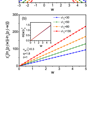
Figure 1: (Color Online) (a) Probability distribution $p_{\tau}(w)$ for the superstatistical model, Eq. (51), for different times $\tau.$ The inset details the peak region. (b) Plot of $\mathit{z}_{q}^{\tau}\{\ln_{q}[p_{\tau}(w)]-\ln_{q}[p_{\tau}(-w)]\}$ for each time $\tau.$ The inset shows the collapse of these curves to a single line when plotting the normalized FR symmetry $\Phi(w)\equiv\mathit{z}_{q}^{\tau}\{\ln_{q}[p_{\tau}(w)]-\ln_{q}[p_{\tau}(-w)]\}/\tau^{\delta},$ Eq. (53). The potential velocity is constant, $a_{c}=0,$ Eq. (41). Hence, $\delta=1,$ Eq. (55). In the natural units of the problem (see text) the parameters are $v_{\ast}=\gamma=k=1.$ The average temperature is $\beta_{0}\gamma v_{\ast}^{2}/k=\alpha_{ph}\tau_{0}=0.3,$ and $q=1.8,$ [Eq.(47)].

In Fig. 1(a) we plot the q-Gaussian distribution (51) for different times $\tau.$ In the inset we show the peaks of the distributions. Their wide diminish with time. We assumed a constant potential’s velocity; $a_{c}=0$ in Eq. (41). Hence, $\delta=1.$ By using the (natural) units of mass $m_{0}=\gamma^{2}/k,$ distance $x_{0}=v_{\ast}\gamma/k,$ and time $\tau_{0}=\gamma/k,$ it follows $\gamma=k=v_{\ast}=1.$ Therefore, the unique free parameters are $q$ [Eq. (47)] and the (dimensionless) noise intensity, that is, the average temperature of the distribution (44), $\beta_{0}(\gamma v_{\ast})^{2}/k=\alpha_{ph}\tau_{0}.$

In Fig. 1(b) we plot the dependence with $w$ of $\mathit{z}_{q}^{\tau}\{\ln_{q}[p_{\tau}(w)]-\ln_{q}[p_{\tau}(-w)]\}.$ The index $q$ is the same that defines the q-Gaussian distribution of Fig. 1(a). For each time, a linear behavior is evident. In the inset we show the collapse to a single line when introducing the time normalization factor $(1/\tau^{\delta}),$ Eq. (53).

In the unnormalized scheme [Eq. (21)], the FR reads

$$\frac{1}{\tau^{\eta}}\{\ln_{q}[p_{\tau}(w)]-\ln_{q}[p_{\tau}(-w)]\}\asymp\frac{[\beta_{q}M_{\tau}]^{\frac{3-q}{2}}}{\tau^{\eta}(2\mathcal{N}_{q})^{1-q}}\asymp\alpha w,$$ (56)

where the coefficients are

$$\alpha=\frac{1}{(2\mathcal{N}_{q})^{1-q}}\Big{(}\frac{\beta_{q}\gamma v_{\ast}^{2}}{1+2a_{c}}\Big{)}^{\frac{3-q}{2}},\ \ \ \ \ \ \ \ \eta=\delta\Big{(}\frac{3-q}{2}\Big{)}.$$ (57)

Here, the coefficient $\alpha$ does not have a clear physical meaning. Nevertheless, as commented before, based on a large deviation-like theory (Appendixes) it is possible to establish some general relations between $\alpha$ and $\alpha_{ph,}$ as well as between $\eta$ and $\delta$ [Eqs. (74) and (98)], which are satisfied in the present case.

III.3 Lévy noise model

In Ref. cohenRapid the noise $\xi(t)$ was taken as a symmetric stable Lévy noise. Furthermore, different experimental setups where the model may be explicitly measured were proposed. While the analysis presented in that contribution is completely right, here we study the same problem by using the generalized FR. We explicitly show that a FR can be established only when the probabilities satisfy a LDP.

The noise is defined by its characteristic functional

$$G_{\xi}[\lambda(t)] = \Big{\langle}\exp i\int_{0}^{\infty}dt\lambda(t)\xi(t)\Big{\rangle},$$ (58a)

$$= \exp\Big{(}-b\int_{0}^{\infty}dt|\lambda(t)|^{\sigma}\Big{)},$$ (58b)

where $$\lambda(t) b 0<\sigma<2. \sigma. G_{W}(\lambda)=\int_{-\infty}^{+\infty}dWP_{\tau}(W)\exp[i\lambda W],$$ is an arbitrary test function. The constant measures the noise intensity and Due to the linearity of the stochastic dynamics (29), the work (30) is also a stable variable with the same index It characteristic function, then reads

$$G_{W}(\lambda) = \langle\exp[i\lambda W_{\tau}]\rangle,$$ (59a)

$$= \exp(iM_{\tau}\lambda-B_{\tau}\left|\lambda\right|^{\sigma}),$$ (59b)

where $$M_{\tau} B_{\tau} G_{W}(\lambda) G_{\xi}[\lambda(t)]. v^{\ast}(t),$$ is defined by Eq. (31) and can be obtained after writing in terms of For arbitrary velocities we get

$$B_{\tau}=b\Big{(}\frac{k}{\gamma}\Big{)}^{\sigma}\int_{0}^{\tau}dt\left|\int_{t}^{\tau}dt^{\prime}e^{-(t^{\prime}-t)/\tau_{0}}v^{\ast}(t^{\prime})\right|^{\sigma}.$$ (60)

For $\tau\gg\tau_{0},$ $M_{\tau}$ can be calculated from Eq. (33), while $B_{\tau},$ after taking $e^{-(t^{\prime}-t)/\tau_{0}}\asymp\tau_{0}\delta(t^{\prime}-t),$ can be approximated as

$$B_{\tau}\asymp b\int_{0}^{\tau}dt\left|v^{\ast}(t)\right|^{\sigma}.$$ (61)

Eq. (59) corresponds to the Fourier transform of a Lévy probability distribution. As is well known levyNum , for $|W-M_{\tau}|\gtrsim B_{\tau}^{1/\sigma}$ it develops power-law tails,

$$P_{\tau}(W)\approx\frac{c_{\sigma}B_{\tau}}{|W-M_{\tau}|^{1+\sigma}},$$ (62)

where $c_{\sigma}=\pi^{-1}\sigma\sin(\pi\sigma/2)\Gamma(\sigma).$ Only when $\sigma=1,$ one gets a simple analytical expression valid for any value of $W,$ $P_{\tau}(W)=(V_{\tau}/\pi)[(W-M_{\tau})^{2}+V_{\tau}^{2}]^{-1}.$ It is expected that Eq. (62) satisfies the normalized FR

$$\mathcal{Z}_{q}^{\tau}\{\ln_{q}[P_{\tau}(W)]-\ln_{q}[P_{\tau}(-W)]\}\propto\zeta_{ph}(\tau)W,$$ (63)

where the symbol $\propto$ denotes both an asymptotic time regime $(\tau\gg\tau_{0})$ and $|W-M_{\tau}|\gtrsim B_{\tau}^{1/\sigma},$ that is, values of $W$ in the power-law regime. The parameter $q$ and the function $\zeta_{ph}(\tau)$ can be found by mapping the approximation (62) with the power-law behavior of the q-Gaussian distribution (45). We get

$$q=\frac{\sigma+3}{\sigma+1},\ \ \ \ \ \ \ \ \ V_{\tau}=c_{\sigma}^{\prime}B_{\tau}^{\frac{2}{\sigma}}.$$ (64)

where $c_{\sigma}^{\prime}=\frac{1}{2}(\frac{2}{1+\sigma})^{\frac{1+\sigma}{\sigma}}(c_{\sigma}\mathcal{N}_{q})^{\frac{2}{\sigma}}.$ Notice that $5/3<q<3$ LevyAsQ . With these relations at hand, the time dependent function $\zeta(\tau)$ reads

$$\zeta_{ph}(\tau)\approx c_{\sigma}^{\prime\prime}\frac{\gamma}{b^{\frac{2}{\sigma}}}\frac{1}{\tau^{\frac{2}{\sigma}-1}}.$$ (65)

with $c_{\sigma}^{\prime\prime}=\frac{2}{c_{\sigma}^{\prime}}\frac{\sigma}{1+\sigma}\frac{(1+a_{c}\sigma)^{\frac{2}{\sigma}}}{1+2a_{c}}.$ In deriving this expression we assumed the general velocity dependence (41). While in the power-law regime the Lévy distribution satisfy the generalized FR (63), the proportionality constant [Eq. (48)] becomes time dependent, $\zeta_{ph}\rightarrow\zeta_{ph}(\tau).$ At long times, for any value of $\sigma\in(0,2),$ it vanishes. Hence, consistently with the results of Ref. cohenRapid , one conclude that asymptotically positive and negative fluctuations of the same magnitude have the same statistical weight. On the other hand, by comparison with the fluctuation theorem (49), it follows that here it is not possible to associate a temperature to the stochastic Lévy dynamics.

Other distinctive features of the problem can be characterized by analyzing the statistics of the dimensionless work (34). After a simple changes of variables, from Eq. (59), the Fourier transform of its probability $p_{\tau}(w)$ reads

$$G_{w}(\lambda) = \langle\exp[i\lambda w_{\tau}]\rangle,$$ (66a)

$$= \exp(i\lambda w_{0}-\tilde{B}_{\tau}\left|\lambda\right|^{\sigma}),$$ (66b)

where the coefficients are

$$w_{0}=1,\ \ \ \ \ \ \ \ \tilde{B}_{\tau}=\frac{B_{\tau}}{|M_{\tau}|^{\sigma}}.$$ (67)

From Eqs. (33) and (61) we get the asymptotic behavior

$$\tilde{B}_{\tau}\asymp\frac{b}{\gamma^{\sigma}}\frac{\int_{0}^{\tau}dt\left|v^{\ast}(t)\right|^{\sigma}}{\left|\int_{0}^{\tau}dt[v^{\ast}(t)]^{2}\right|^{\sigma}}.$$ (68)

For the velocity dependence (41), it follows

$$\tilde{B}_{\tau}\asymp d_{\sigma}\frac{b}{(\gamma v_{\ast})^{\sigma}}\frac{1}{\tau^{\sigma(1+a_{c})-1}},\ \ \ \ \ \ \ v^{\ast}(t)=v_{\ast}t^{a_{c}}.$$ (69)

where $d_{\sigma}=\frac{(1+2a_{c}\sigma)^{\sigma}}{1+a_{c}\sigma}.$ Therefore, when $\sigma>1/(1+a_{c})$ the width of the distribution diminishes, while for $\sigma<1/(1+a_{c})$ it increases with time. The former behavior is consistent with a LDP [see Eq. (72)]. Therefore, it should be possible to establishes a (generalized) FR symmetry for $p_{\tau}(w).$ In the second case, the typical fluctuations of the scaled work $w_{\tau}$ increase in size at higher times. This anomalous behavior is inconsistent with both a LDP and the law of large numbers cohenRapid . Therefore, we expect that $p_{\tau}(w)$ does not fulfill any FR in this case. On the other hand, by analyzing $p_{\tau}(w)$ through a standard FR, the transition $\sigma\gtrless 1$ $(a_{c}=0)$ leads to the different characteristic behaviors found in Ref. cohenRapid .

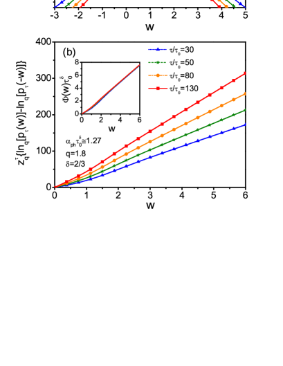
Figure 2: (Color Online) (a) Levy probability distribution $p_{\tau}(w)$ defined by Fourier transform (66) with $\sigma=1.5.$ The inset details the peak region. (b) Plot of $\mathit{z}_{q}^{\tau}\{\ln_{q}[p_{\tau}(w)]-\ln_{q}[p_{\tau}(-w)]\}$ for each time $\tau.$ The inset shows the collapse of these curves when plotting the normalized FR symmetry $\Phi(w)\equiv\mathit{z}_{q}^{\tau}\{\ln_{q}[p_{\tau}(w)]-\ln_{q}[p_{\tau}(-w)]\}/\tau^{\delta},$ Eq. (70). The potential velocity is constant, $a_{c}=0,$ Eq. (41). Hence, $\delta=2/3,$ Eq. (71). In natural units (see text) the parameters are $v_{\ast}=\gamma=k=1.$ The noise intensity reads $b(\gamma v_{\ast})^{2}=2.$

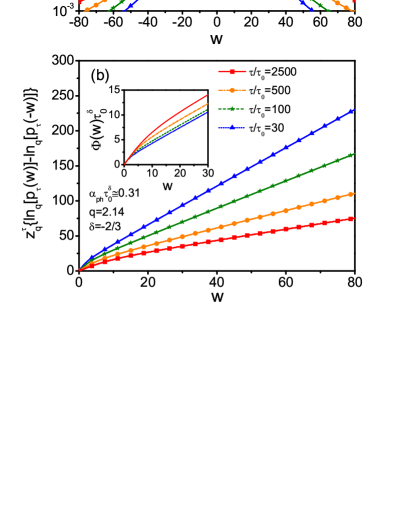
Figure 3: (Color Online) (a) Levy probability distribution $p_{\tau}(w)$ defined by the Fourier transform (66) with $\sigma=0.75.$ The inset details the peak region. (b) Plot of $\mathit{z}_{q}^{\tau}\{\ln_{q}[p_{\tau}(w)]-\ln_{q}[p_{\tau}(-w)]\}$ for each time $\tau.$ The inset corresponds to $\Phi(w)\equiv\mathit{z}_{q}^{\tau}\{\ln_{q}[p_{\tau}(w)]-\ln_{q}[p_{\tau}(-w)]\}/\tau^{\delta},$ Eq. (70). The potential velocity is constant, $a_{c}=0,$ Eq. (41). Hence, $\delta=-2/3<0,$ Eq. (71). In natural units (see text) the parameters are $v_{\ast}=\gamma=k=1.$ The noise intensity reads $b(\gamma v_{\ast})^{2}=2.$

For $|w-w_{0}|\gtrsim\tilde{B}_{\tau}^{1/\sigma},$ the probability distribution $p_{\tau}(w)$ behaves as $p_{\tau}(w)\approx c_{\sigma}\tilde{B}_{\tau}/|w-w_{0}|^{1+\sigma}$ [see Eq. (62)]. In that regime, it satisfies the relation

$$\frac{\mathit{z}_{q}^{\tau}}{\tau^{\delta}}\{\ln_{q}[p_{\tau}(w)]-\ln_{q}[p_{\tau}(-w)]\}\propto\alpha_{ph}w,$$ (70)

where the coefficients read

$$\delta=2(1+a_{c}-\sigma^{-1}),\ \ \ \ \ \ \ \ \alpha_{ph}\approx d_{\sigma}^{\prime}b^{-\frac{2}{\sigma}}(\gamma v_{\ast})^{2},$$ (71)

with $d_{\sigma}^{\prime}=\frac{2\sigma}{1+\sigma}(c_{\sigma}^{\prime}d_{\sigma}^{2/\sigma})^{-1},$ and $q$ is defined by Eq. (64), that is, $q=\frac{\sigma+3}{\sigma+1}.$ On the other hand, the expression for $\alpha_{ph}$ is only approximated because it is based on a mapping with a q-Gaussian distribution. In general, the value of $\mathit{z}_{q}^{\tau},$ Eq. (54), differs from that corresponding to a Lévy distribution.

Eq. (70) is valid for any value of $\sigma\in(0,2)$ if $w$ pertains to the power-law domain. Equivalently, it does not applies for $|w-w_{0}|\lesssim\tilde{B}_{\tau}^{1/\sigma}.$ Therefore, when $\tilde{B}_{\tau}$ decrease (increase) in time the FR symmetry is valid (not valid) for almost any value of $w.$ In fact, the transition in the behavior of the characteristic width $\tilde{B}_{\tau},$ Eq. (69), also determines when a LDP applies $(\delta>0)$ or not $(\delta<0).$ From Eq. (71) it follows $\delta\gtrless 0$ if $\sigma\gtrless 1/(1+a_{c}).$ These properties are explicitly shown in the next figures.

In Fig. 2(a) we plot the (exact numeric) Lévy distribution $p_{\tau}(w)$ levyNum obtained from its Fourier transform (66). We assumed a constant potential’s velocity, $a_{c}=0$ in Eq. (41), and $\sigma=1.5.$ Hence, $q=1.8$ [Eq. (64)], and $\delta=2/3>0$ [Eq. (71)]. Consistently, the peaks around $w=1$ diminish their wide for higher times. By using natural units, the unique free parameter is the (dimensionless) noise intensity [Eq. (58)], $b\tau_{0}(\gamma^{2}v_{\ast}/k)^{-\sigma}.$

In Fig. 2(b) we plot the dependence with $w$ of $\mathit{z}_{q}^{\tau}\{\ln_{q}[p_{\tau}(w)]-\ln_{q}[p_{\tau}(-w)]\}$ for different times $\tau.$ Small deviations with respect to a linear behavior are observed around $|w_{0}-\tilde{B}_{\tau}^{1/\sigma}|<w<|w_{0}+\tilde{B}_{\tau}^{1/\sigma}|.$ Their magnitude diminish with time. In the inset we show the collapse to a single curve when introducing the time normalization factor $(1/\tau^{\delta}),$ Eq. (70). We checked that the same property is valid for higher times, indicating the consistence between the generalized FR and its associated LDP. The value of $\alpha_{ph}\tau_{0}^{\delta}$ was estimated from the slope of the collapsed curves (inset). The theoretical estimation, Eq. (71), gives $\alpha_{ph}\tau_{0}^{\delta}=1.85.$

In Fig. 3(a) we plot the Lévy distribution $p_{\tau}(w)$ for $\sigma=0.75,$ and $a_{c}=0.$ Hence, $q=15/7\simeq 2.14$ [Eq. (64)], and $\delta=-2/3<0$ [Eq. (71)]. A negative $\delta$ implies that the wide of the peaks around $w=1$ grows with time. The linear behavior of $\mathit{z}_{q}^{\tau}\{\ln_{q}[p_{\tau}(w)]-\ln_{q}[p_{\tau}(-w)]\}$ with $w$ is only valid for $w\gtrsim w_{0}+\tilde{B}_{\tau}^{1/\sigma},$ where $\tilde{B}_{\tau}$ increases in time. Added to this failure, after introducing the normalization factor $(1/\tau^{\delta}),$ the curves does not collapse into a single curve (inset). These properties are parallel to the inapplicability of a LDP. On the other hand, the theoretical estimation, Eq. (71), gives $\alpha_{ph}\tau_{0}^{\delta}=0.21.$

IV Summary and Conclusions

We have introduced an alternative definition of FR symmetry that satisfies two conditions. In the regime where the probability of interest develops power-law tails the symmetry is expressed through a linear behavior. Furthermore, the generalized symmetry has associated a large deviation-like theory.

The FR symmetry can be written as a difference between the generalized q-logarithm of the probability distributions for positive and negative fluctuations, Eq. (6). The parameter $q$ depends on the exponent of the power-law tails. In terms of a generalized characteristic function, Eq. (9), the proposed FR can be expressed as in the standard case, Eq. (10). Similar relations, Eqs. (21) and (25), were formulated for time-scaled variables. Based on large deviation-like principle, in the Appendixes we showed that a set of LDFs can be consistently defined for both the probability distribution and its associated characteristic function. The standard Legendre structure connecting them remains valid even in presence of self-similar power-law distributions, Eqs. (94) and (95). Therefore, the generalized FR can be expressed as in the standard case when written in term of the LDFs, Eqs. (96) and (97).

The general formalism was applied for characterizing the fluctuations of the work performed on a dragged particle immersed in a complex environment. When the power-law nature of the dynamics is induced by (spaciotemporal) temperature fluctuations, the work statistics is given by a q-Gaussian distribution. The FR symmetry is scaled by the environment average temperature. This novel fluctuation theorem [Eq. (49)] may in principle be confirmed in different experimental setups beckQ .

By analyzing the case in which the environment is represented by an external Lévy noise, we reinterpreted the results of Ref. cohenRapid . Taking into account the superstatistical model, we conclude that some of those results are not valid in general. Due to the interplay between the noise statistics, the velocity of the power input, and the particle dissipative dynamics, in the long time regime the probabilities of positive and negative fluctuations of equal magnitude become identical. This result follows from the asymptotic vanishing of the characteristic constant that defines the work probability symmetry, Eqs. (63) and (65). On the other hand, the time-scaled work only satisfies the generalized FR when its behavior is compatible with a LDP, that is, the size of its characteristic fluctuations must to diminish with time (Fig. 2 and 3).

While the uniqueness of the present proposal was not proved, based on the requirements that it satisfies unico , one can conclude that it may be considered as a valid and solid tool for analyzing nonequilibrium fluctuations in systems characterized by power-law distributions. The stretched relation with nonextensive thermodynamics TsallisBook , as well as its applicability in specific experimental setups NanoSuperFT are open problems that with certainty deserve extra analysis.

Appendix A Large deviation functions

In this Section it is shown the consistence of the proposed FR with a large deviation-like principle. It is not obvious that an arbitrary generalized FR may satisfies this condition. Specifically, we show that it is possible to define two LDFs from the (long time) asymptotic behavior of the probability density and its associated q-characteristic function. Both of them become related by a Legendre-Fenchel transformation touchette . These results provide a solid mathematical support to the proposed FR.

A.1 Unnormalized scheme

We base our analysis on time-scaled variables, Eq. (20). A large deviation-like principle relies on providing a general structure for the probability $p(\mu)$ in the long time regime. Instead of a standard exponential structure touchette , here we assume

$$p(\mu)\asymp\frac{t^{\delta/2}}{C_{q}}\exp_{q}[-t^{\delta}C_{q}^{1-q}\varphi(\mu)].$$ (72)

As before, the symbol $\asymp$ denotes an equality valid in a long time regime. The factor $t^{\delta}$ $(\delta>0)$ measures the time-speed of $\varphi(\mu)\geq 0.$ As in Refs. klages ; harris (see also Appendix D of Ref. touchette ), we consider the case in which $\delta\neq 1.$ On the other hand, the factor $(t^{\delta/2}/C_{q})$ in front of the q-exponential is necessary for providing the rights units and normalization of $p(\mu).$

After a simple manipulation without involving any extra approximation, Eq. (72) can be rewritten as

$$p(\mu)\asymp\frac{t^{\delta/2}}{C_{q}}\otimes_{q}\exp_{q}[-t^{\eta}\varphi(\mu)],$$ (73)

where the exponent $\eta$ reads

$$\eta=\delta\Big{(}\frac{3-q}{2}\Big{)}.$$ (74)

Written is this way, given that $\lim_{t\rightarrow\infty}\ln_{q}[t^{\delta/2}/C_{q}]/t^{\eta}=0,$ the function $\varphi(\mu)$ can be obtained as

$$\varphi(\mu)=\lim_{t\rightarrow\infty}\frac{-1}{t^{\eta}}\ln_{q}[p(\mu)].$$ (75)

Hence, it can be read as the probability’s LDF touchette .

Another LDF can be defined from the asymptotic time behavior of $Z_{q}(\lambda).$ Its structure can be obtained from the definition (23), after taking into account the probability asymptotic behavior (72). In general, the resulting integral cannot be obtained exactly. Nevertheless, it can be worked out through a steepest descent approximation. In Appendix B we derive the asymptotic expression

$$Z_{q}(\lambda)\asymp\exp_{\tilde{q}}\Big{[}-\Big{(}\frac{3-q}{2}\Big{)}t^{\delta}C_{q}^{1-q}\Theta(\lambda)\Big{]},$$ (76)

where the index of the q-exponential reads

$$\tilde{q}=\frac{1+q}{3-q}.$$ (77)

Hence, the LDF associated to $Z_{q}(\lambda)$ can be defined as

$$\Theta(\lambda)=\lim_{t\rightarrow\infty}\frac{-1}{t^{\delta}}\frac{2}{(3-q)}C_{q}^{q-1}\ln_{\tilde{q}}[Z_{q}(\lambda)].$$ (78)

The steepest descent approximation establishes a link between both LDF (Appendix B). They are related by the Legendre-Fenchel transformation

$$\Theta(\lambda)=\min_{\mu}[\varphi(\mu)+\lambda\mu],$$ (79)

jointly with the inverse equation

$$\varphi(\mu)=\max_{\lambda}[\Theta(\lambda)-\lambda\mu].$$ (80)

These relations also arise from a standard LDP, where the asymptotic behavior of the probability and its characteristic function scales with standard exponential functions. Remarkably, this Legendre structure remains valid even when the distributions develop power-law tails.

A.1.1 Symmetries of the LDFs

After establishing a large deviation-like principle [Eqs. (73) and (76)], we ask about the symmetries that the LDFs must to satisfy when the generalized FR is valid in the long time regime. A probability $p(\mu),$ with the asymptotic structure (73), satisfies the FR (21) if the LDF $\varphi(\mu)$ fulfill the condition

$$-\varphi(\mu)+\varphi(-\mu)=\alpha\mu.$$ (81)

Furthermore, the characteristic function (76) satisfies the symmetry (24) if the LDF $\Theta(\lambda)$ satisfies

$$\Theta(\lambda)=\Theta(-\lambda+\alpha).$$ (82)

Both conditions are consistent between them. In fact, one can be derived from the other by using the Legendre structure defined by Eqs. (79) and (80). The demonstration is exactly the same than in the standard case spohn ; mukamel .

A.1.2 q-Gaussian distribution

It is very instructive to exemplify the previous results with an arbitrary q-Gaussian distributed variable. Let consider a stochastic variable $x_{st}(t)$ whose long time statistics is given by Eq. (13) under the replacements $x_{0}\rightarrow x_{0}(t)$ and $\beta\rightarrow\beta(t).$ Furthermore, we assume that asymptotically these objects behave as

$$x_{0}(t)\asymp\mu_{0}t^{\kappa},\ \ \ \ \ \ \ \ \ \beta(t)\asymp\frac{\Delta_{0}}{t^{\kappa^{\prime}}}.$$ (83)

Both, $\kappa$ and $\kappa^{\prime}$ are positive exponents, while $\mu_{0}$ and $\Delta_{0}$ are characteristic constants. Notice that both the average (strictly the most probable value) and the characteristic width of the distribution $p(x)$ grows with time.

By defining $\mu_{st}(t)=x_{st}(t)/t^{\kappa}$ [Eq. (20)], using the change of measures $p(\mu)d\mu=p(x)dx,$ from Eq. (13) it follows the distribution

$$p(\mu)\asymp\frac{\sqrt{\Delta_{0}t^{2\kappa-\kappa^{\prime}}}}{\mathcal{N}_{q}}\exp_{q}[-\Delta_{0}t^{2\kappa-\kappa^{\prime}}(\mu-\mu_{0})^{2}].$$ (84)

Hence, by comparing with Eq. (72) it follow the identifications

$$\delta=2\kappa-\kappa^{\prime},\ \ \ \ \ \ \ \ \ C_{q}=\frac{\mathcal{N}_{q}}{\sqrt{\Delta_{0}}}.$$ (85)

The probability LDF reads

$$\varphi(\mu)=\frac{(\Delta_{0})^{\frac{3-q}{2}}}{\mathcal{N}_{q}^{1-q}}(\mu-\mu_{0})^{2}.$$ (86)

In order to be consistent with a LDP, the exponent $\delta$ must be positive, $2\kappa>\kappa^{\prime}.$ Hence, the width of the distribution $p(\mu)$ diminishes with time. This property is expected for a time-scaled variable, Eq. (20). A common situation corresponds to $\kappa=\kappa^{\prime}=1$ giving $\delta=1.$ Even in this case, the exponent $\eta,$ Eq. (74), which defines the limit (75), is different from one for $q\neq 1.$

The q-characteristic function (23) associated to the distribution (84) can be obtained exactly by using the previous result (17). After a simple change of variables, we get

$$Z_{q}(\lambda)\asymp\exp_{\tilde{q}}\Big{\{}\Big{(}\frac{3-q}{2}\Big{)}t^{\delta}C_{q}^{1-q}\Big{[}\frac{\lambda^{2}\mathcal{N}_{q}^{1-q}}{4(\Delta_{0})^{\frac{3-q}{2}}}-\lambda\mu_{0}\Big{]}\Big{\}},$$ (87)

where $\tilde{q}$ is given by Eq. (18), $\delta$ and $C_{q}$ by Eq. (85). We notice that this structure corresponds to that obtained from a steeps descent integration, Eq. (76). In fact, that approximation is exact for a q-Gaussian distribution.

By comparing Eq. (76) and (87), we obtain the LDF $\Theta(\lambda).$ It reads

$$\Theta(\lambda)=-\frac{\lambda^{2}\mathcal{N}_{q}^{1-q}}{4(\Delta_{0})^{\frac{3-q}{2}}}+\lambda\mu_{0}.$$ (88)

It is straightforward to prove that $\varphi(\mu)$ [Eq. (86)] and $\Theta(\lambda)$ [Eq. (88)] are related by the Legendre-Fenchel transformations (79) and (80). Furthermore, both LDF satisfy respectively the symmetries (81) and (82) with the same constant $\alpha,$ which reads

$$\alpha=4\mu_{0}\frac{(\Delta_{0})^{\frac{3-q}{2}}}{\mathcal{N}_{q}^{1-q}}.$$ (89)

As expected, when $q\rightarrow 1$ the expressions (86), (88), and (89) reduce to those corresponding to a normal Gaussian distribution.

A.2 Normalized Scheme

Eqs. (81) and (82) are equivalent to the unnormalized FR (21). The normalized FR (25) can also be expressed through a set of renormalized LDFs. We define

$$\varphi^{ph}(\mu)=\lim_{t\rightarrow\infty}\frac{-1}{t^{\delta}}\Big{(}\int_{-\infty}^{\infty}d\mu[p(\mu)]^{q}\Big{)}\ln_{q}[p(\mu)],$$ (90)

and similarly

$$\Theta^{ph}(\lambda_{ph})=\lim_{t\rightarrow\infty}\frac{-1}{t^{\delta}}\ln_{\tilde{q}}[Z_{q}^{ph}(\lambda_{ph})].$$ (91)

In the asymptotic regime, the relation (26) is equivalent to $\lambda_{ph}=\lambda\lim_{t\rightarrow\infty}\frac{1}{t^{\delta-\eta}}\int_{-\infty}^{\infty}d\mu[p(\mu)]^{q}.$ In fact, it is possible to demonstrate that

$$D_{q}^{1-q}\equiv\lim_{t\rightarrow\infty}\frac{1}{t^{\delta-\eta}}\int_{-\infty}^{\infty}d\mu[p(\mu)]^{q}=\Big{(}\frac{3-q}{2}\Big{)}C_{q}^{1-q},$$ (92)

where $(\delta-\eta)=(q-1)\delta/2.$ Hence, $\eta$ is the same exponent defined in Eq. (74). The last equality in Eq. (92) follows by calculating the integral through a steepest descent approximation, where $p(u)$ is given by (72). In the derivation we used the result (111) and the equality $\frac{3-q}{2}=\Gamma(\frac{1}{q-1})\Gamma(\frac{1+q}{2(q-1)})/[\Gamma(\frac{q}{q-1})\Gamma(\frac{3-q}{2(q-1)})].$ By comparing the LDFs corresponding to the unnormalized [Eqs. (75) and (78)] and normalized [(90) and (91)] schemes, from Eq. (92) it follows the relations

$$\varphi^{ph}(\mu)=\frac{\varphi(\mu)}{D_{q}^{q-1}},\ \ \ \ \ \ \ \ \ \ \Theta^{ph}(\lambda_{ph})=\frac{\Theta(\lambda_{ph}D_{q}^{q-1})}{D_{q}^{q-1}}.$$ (93)

Taking into account Legendre-Fenchel transformations (79) and (80), Eq. (93) implies that

$$\Theta^{ph}(\lambda_{ph})=\min_{\mu}[\varphi^{ph}(\mu)+\lambda_{ph}\mu],$$ (94)

jointly with the inverse relation

$$\varphi^{ph}(\mu)=\max_{\lambda_{ph}}[\Theta^{ph}(\lambda_{pj})-\lambda_{ph}\mu].$$ (95)

Therefore, the normalized definitions (90) and (91) also maintain the Legendre structure associated to a large deviation theory.

A.2.1 Symmetries of the LDFs

The (unnormalized) symmetries (81) and (82), added to the relations (93), lead to the equivalent relations

$$-\varphi^{ph}(\mu)+\varphi^{ph}(-\mu)=\alpha^{ph}\mu,$$ (96)

and consistently

$$\Theta^{ph}(\lambda_{ph})=\Theta^{ph}(-\lambda_{ph}+\alpha^{ph}),$$ (97)

where the constant $\alpha_{ph}$ reads

$$\alpha_{ph}=\frac{\alpha}{D_{q}^{q-1}}.$$ (98)

A.2.2 q-Gaussian distribution

For the previous example, defined by the q-Gaussian distribution (84), it follows the LDF

$$\varphi^{ph}(\mu)=\Big{(}\frac{3-q}{2}\Big{)}\Delta_{0}(\mu-\mu_{0})^{2}.$$ (99)

The q-characteristic function (87) leads to

$$Z_{q}^{ph}(\lambda_{ph})\asymp\exp_{\tilde{q}}\Big{\{}t^{\delta}\Big{[}\frac{\lambda_{ph}^{2}}{4(\frac{3-q}{2})\Delta_{0}}-\lambda_{ph}\mu_{0}\Big{]}\Big{\}}.$$ (100)

Therefore, we get

$$\Theta^{ph}(\lambda_{ph})=-\frac{\lambda_{ph}^{2}}{4(\frac{3-q}{2})\Delta_{0}}+\lambda_{ph}\mu_{0}.$$ (101)

The constant $\alpha_{ph}$ reads

$$\alpha_{ph}=4\mu_{0}\Delta_{0}\Big{(}\frac{3-q}{2}\Big{)}.$$ (102)

Notice that all dependences of the LDFs with the parameter $q$ can be absorbed in the coefficient $\Delta_{0}.$

Appendix B Steepest descent approximation

Here we develop a set of approximations that allow to calculate the long time behavior of $Z_{q}(\lambda)$ from the asymptotic behavior of $p(\mu).$ The procedure is similar to that given in Refs. mukamel (see Appendix C) and touchette .

By introducing (72) in Eq. (23), after some calculations steps, we get

$$Z_{q}(\lambda)\asymp\frac{t^{\delta/2}}{C_{q}}\int_{-\infty}^{\infty}d\mu\exp_{q}\{-t^{\delta}C_{q}^{1-q}[\varphi(\mu)+\lambda\mu]\}.$$ (103)

This integral cannot be performed in an exact way. In order to proceed, we introduce an integral representation of the q-exponential function $(q>1)$ TsallisBook ; stepestQ

$$e_{q}^{-z}=\frac{1}{\Gamma(\frac{1}{q-1})}\int_{0}^{\infty}d\tau\tau^{\frac{2-q}{q-1}}e^{-\tau[1+(q-1)z]},$$ (104)

$(z>0).$ Hence, after inverting the order of the integrals, we write

$$Z_{q}(\lambda) \asymp \frac{t^{\delta/2}}{\Gamma(\frac{1}{q-1})C_{q}}\int_{0}^{\infty}d\tau\tau^{\frac{2-q}{q-1}}e^{-\tau}\int_{-\infty}^{\infty}d\mu$$

$$\times\exp\{-t^{\delta}\tau[\varphi(\mu)+\lambda\mu]C_{q}^{1-q}(q-1)\}.$$

At long times $t,$ the integral in the $\mu$ variable can be worked out with a steepest descent integration method. The main contribution to the integral comes from the value of $\mu,$ $\mu^{\ast},$ that minimizes the exponential. Defining $\mu^{\ast}=\mu^{\ast}(\lambda)$ by the condition $\dot{\varphi}(\mu^{\ast})=-\lambda,$ $[\dot{\varphi}(z)=(d/dz)\varphi(z)],$ we can approximate

$$\varphi(\mu)+\lambda\mu\approx\varphi(\mu^{\ast})+\lambda\mu^{\ast}+\frac{1}{2}\ddot{\varphi}(\mu^{\ast})(\mu-\mu^{\ast})^{2}.$$ (106)

By assuming that $\varphi(\mu)$ is a convex function to have a minimum, $\ddot{\varphi}(\mu^{\ast})>0,$ and using the integral $\int_{-\infty}^{\infty}d\mu e^{-a\mu^{2}}=(\pi/a)^{1/2},$ it follows

$$Z_{q}(\lambda) \asymp \frac{1}{\Gamma(\frac{1}{q-1})C_{q}^{\frac{3-q}{2}}}\frac{\sqrt{2\pi}}{\sqrt{(q-1)\ddot{\varphi}(\mu^{\ast})}}$$

$$\times\int_{0}^{\infty}d\tau\tau^{(\frac{2-q}{q-1}-\frac{1}{2})}e^{\{-\tau[1+t^{\delta}\Theta(\lambda)C_{q}^{1-q}(q-1)]\}}.$$

Here, $\Theta(\lambda)$ denote the function

$$\Theta(\lambda)=\varphi(\mu)+\lambda\mu,$$ (108)

where the value of $\mu$ follows from the condition

$$\dot{\varphi}(\mu)=-\lambda.$$ (109)

By using again the integral representation (104), we arrive to the expression

$$Z_{q}(\lambda)\asymp A_{q}\exp_{\tilde{q}}\Big{[}-\Big{(}\frac{3-q}{2}\Big{)}t^{\delta}C_{q}^{1-q}\Theta(\lambda)\Big{]},$$ (110)

where $\tilde{q}$ is given by Eq. (77), $\tilde{q}=(1+q)/(3-q).$ The constant $A_{q}$ is

$$A_{q}\!=\!\frac{\Gamma(\frac{1}{\tilde{q}-1})\sqrt{2\pi}}{\Gamma(\frac{1}{q-1})C_{q}^{\frac{3-q}{2}}\sqrt{(q-1)\ddot{\varphi}(\mu^{\ast})}}\!=\!\frac{\mathcal{N}_{q}}{C_{q}^{\frac{3-q}{2}}}\sqrt{\frac{2}{\ddot{\varphi}(\mu^{\ast})}}\!\simeq\!1.$$ (111)

Therefore, Eq. (110) leads to the expression (76). In the previous expression, the second equality follows from Eq. (14), while the last estimation follows by applying a steepest descent approximation to the condition $\int_{-\infty}^{+\infty}d\mu p(u)\asymp 1,$ where $p(u)$ is given by (72), jointly with the condition that the LDF $\varphi(\mu)$ vanishes at its minimum $\mu_{\min},$ $\varphi(\mu_{\min})=0,$ which consistently implies $\Theta(0)=0,$ $Z_{q}(0)\asymp 1.$

Eqs. (108) and (109) show that $\Theta(\lambda)$ is the Legendre transform of $\varphi(\mu),$ which in turn can be written as in Eq. (79). On the other hand, the derivative of $\Theta(\lambda)$ with respect to $\lambda$ is

$$\dot{\Theta}(\lambda)=\dot{\varphi}(\mu)\frac{d\mu}{d\lambda}+\mu+\lambda\frac{d\mu}{d\lambda},$$ (112)

which from Eq. (109) leads to

$$\dot{\Theta}(\lambda)=\mu.$$ (113)

This shows that $\varphi(\mu)$ is given by the inverse Legendre transform of $\Theta(\lambda),$

$$\varphi(\mu)=\Theta(\lambda)-\lambda\mu.$$ (114)

Here the value of $\lambda$ follows from the condition (113), leading to Eq. (80). In fact, by taking the derivative of (113) with respect to $\lambda$ and using the derivative of (109) with respect to $\mu$ we can confirm that $\varphi(\mu)$ is convex because $\Theta(\lambda)$ is concave, $\ddot{\varphi}(\mu)=-1/\ddot{\Theta}(\lambda).$

References

- (1) G. Gallavotti and E.G.D. Cohen, Phys. Rev. Lett. 74, 2694 (1995); D.J. Evans, E.G.D. Cohen, and G.P. Morris, Phys. Rev. Lett. 71, 2401 (1993).
- (2) C. Jarzynski, Phys. Rev. Lett. 78, 2690 (1997).
- (3) J. Kurchan, J. Phys. A 31, 3719 (1998).
- (4) J.L. Lebowitz and H. Spohn, J. Stat. Phys. 95, 333 (1999).
- (5) G.E. Crocks, Phys. Rev. E 60, 2721 (1999).
- (6) C. Maes, J. Stat. Phys. 95, 367 (1999).
- (7) U. Seifert, Phys. Rev. Lett. 95, 040602 (2005).
- (8) E.M. Sevick, R. Prabhakar, S.R. Williams, and D.J. Searles, Annu. Rev. Phys. Chem 59, 603 (2008).
- (9) U.M.B. Marconi, A. Puglisi, L. Rondoni, and A. Vulpiani, Phys. Rep. 461, 111 (2008).
- (10) M. Esposito, U. Harbola, and S. Mukamel, Rev. Mod. Phys. 81, 1665 (2009).
- (11) C. Jarzynski, Annu. Rev. Condens. Matter Phys. 2, 329 (2011).
- (12) W.I. Goldburg, Y.Y. Goldschmidt, and H. Kellay, Phys. Rev. Lett. 87, 245502 (2001); D.M. Carberry, J.C. Reid, G.M. Wang, E.M. Sevick, D.J. Searles, and D.J. Evans, Phys. Rev. Lett. 92, 140601 (2004); A. Puglisi, P. Visco, A. Barrat, E. Trizac, and F. van Wijland, Phys. Rev. Lett. 95, 110202 (2005); S. Schuler, T. Speck, C. Tietz, J. Wrachtrup, and U. Siefert, Phys. Rev. Lett. 94, 180602 (2005); M. Belushkin, R. Livi, and G. Foffi, Phys. Rev. Lett. 106, 210601 (2011).
- (13) A.A. Budini, Phys. Rev. E 84, 061118 (2011); N. Kumar, S. Ramaswamy, and A.K. Sood, Phys. Rev. Lett. 106, 118001 (2011).
- (14) O. Mazonka and C. Jarzynski, arXiv:cond-mat/9912121 (1999).
- (15) R. van Zon and E.G.D. Cohen, Phys. Rev. E 67, 046102 (2003).
- (16) G.M. Wang, E.M. Sevick, E. Mittag, D.J. Searles, and D.J. Evans, Phys. Rev. Lett. 89, 050601 (2002).
- (17) R. van Zon and E.G.D. Cohen, Phys. Rev. Lett. 91, 110601 (2003); Phys. Rev. E 69, 056121 (2004).
- (18) A. Baule and E.G.D. Cohen, Phys. Rev. E 79, 030103(R) (2009); Phys. Rev. E, 80, 011110 (2009).
- (19) J.R. Gomez-Solano, L. Bellon, A. Petrosyan, and S. Ciliberto, EPL 89, 60003 (2010); M. Bonaldi, et. al., Phys. Rev. Lett. 103, 010601 (2009); C. Falcon and E. Falcon, Phys. Rev. E 79, 041110 (2009); E. Falcon, S. Aumaitre, C. Falcon, C. Laroche, and S. Fauve, Phys. Rev. Lett. 100, 064503 (2008); Jean Farago, J. Stat. Phys. 107, 781 (2002).
- (20) H. Touchette, Phys. Rep. 478, 1 (2009).
- (21) D. Sornette, Critical Phenomena in Natural Sciences, (Springer, 2006).
- (22) L.O. Hedges, R.L. Jack, J.P. Garrahan, and D. Chandler, Science 323, 1309 (2009); J.P. Garrahan and I. Lesanovsky, Phys. Rev. Lett. 104, 160601 (2010); J.P. Garrahan, A.D. Armour, and I. Lesanovsky, Phys. Rev. E 84, 021115 (2011); A.A. Budini, Phys. Rev. E 82, 061106 (2010); Phys. Rev. E 84, 011141 (2011).
- (23) H. Touchette and E.G.D. Cohen, Phys. Rev. E 76, 020101(R) (2007); Phys. Rev. E 80, 011114 (2009).
- (24) A.V. Chechkin and R. Klages, J. Stat. Mech.: Theory Exp. (2009), L03002.
- (25) R.J. Harris and H. Touchette, J. Phys. A 42, 342001 (2009).
- (26) C. Beck and E.G.D. Cohen, Phys. A 344, 393 (2004).
- (27) C. Beck, Phys. Rev. Lett. 87, 180601 (2001).
- (28) C. Beck and E.G.D. Cohen, Phys. A 322, 267 (2003); H. Touchette and C. Beck, Phys. Rev. E 71, 016131 (2005); S. Abe, C. Beck, and E.G.D. Cohen, Phys. Rev. E 76, 031102 (2007).
- (29) C. Tsallis, Introduction to Nonextensive Statistical Mechanics, (Springer, 2009).
- (30) M. Sugiyama, ed., Nonadditive Entropy and Nonextensive Statistical Mechanics, Continuum Mechanics and Thermodynamics 16 (Springer-Verlag, Heidelberg, 2004); P. Grigolini, C. Tsallis, and B.J. West, eds., Classical and Quantum Complexity and Nonextensive Thermodynamics, Chaos, Solitons and Fractals 13, Issue 3 (2002); S. Abe and Y. Okamoto, eds., Nonextensive Statistical Mechanics and its Applications, Series Lecture Notes in Physics 560 (Springer, Berlin, 2001).
- (31) S. Umarov, C. Tsallis, and S. Steinberg, Milan J. Math. 76, 307 (2008); A. Rodriguez, V. Schwämmle, and C. Tsallis, J. Stat. Mech.: Theory Exp. (2008), P09006; R. Hanel, S. Thurner, and C. Tsallis, Eur. Phys. J. B 72, 263 (2009).
- (32) C. Tsallis and D.J. Bukman, Phys. Rev. E 54, R2197 (1996); M. Bologna, C. Tsallis, and P. Grigolini, Phys. Rev. E 62, 2213 (2000).
- (33) C. Tsallis, R.S. Mendes, and A.R. Plastino, Phys. A 261, 534 (1998).
- (34) D. Prato and C. Tsallis, Phys. Rev. E 60, 2398 (1999); C. Tsallis, S.V.F. Levy, A.M.C. Souza, and R. Maynard, Phys. Rev. Lett. 75, 3589 (1995).
- (35) S. Abe and A.K. Rajagopal, J. Phys. A 33, 8733 (2000).
- (36) V. Garcia-Morales and K. Krischer, Proc. Natl. Acad. Sci. U.S.A. 108, 19535 (2011).
- (37) R.H. Rimmer and J.P. Nolan, Math. J. 9, 776 (2005).
- (38) Different generalizations of the logarithmic function kania may be the basis for proposing alternative FRs. Nevertheless, it is not clear at this point if any alternative definition can satisfy the properties of the present approach: (i) The FR must be expressed by a linear dependence when power-law arises. (ii) It must be possible to define the symmetry in terms of a characteristic-like function. (iii) The long time behavior of the probability and its characteristic function must be defined in terms of a set of LDF’s related by a Legendre transform.
- (39) P. Tempesta, Phys. Rev. E 84, 021121 (2011); S. Umarov, C. Tsallis, M. Gell-Mann, and S. Steinberg, J. Math. Phys. 51, 033502 (2010).