Magnetism in parent Fe-chalcogenides: quantum fluctuations select a plaquette order

Abstract

We analyze magnetic order in iron-chalcogenide Fe_1+yTe – the parent compound of high-temperature superconductor Fe_1+yTe_1-xSe_x. Neutron scattering experiments show that magnetic order in this material contains components with momentum $Q_{1}=(\pi/2,\pi/2)$ and $Q_{2}=(\pi/2,-\pi/2)$ in Fe-only Brillouin zone. The actual spin order depends on the interplay between these two components. Previous works argued that spin order is a single-$Q$ state (either $Q_{1}$ or $Q_{2}$). Such an order breaks rotational $C_{4}$ symmetry and order spins into a double diagonal stripe. We show that quantum fluctuations actually select another order – a double $Q$ plaquette state with equal weight of $Q_{1}$ and $Q_{2}$ components, which preserves $C_{4}$ symmetry but breaks $Z_{4}$ translational symmetry. We argue that the plaquette state is consistent with recent neutron scattering experiments on Fe_1+yTe.

Introduction. The analysis of magnetism in parent compounds of iron-based superconductors (FeSCs) is an integral part of the program to understand the origin of superconductivity in these materials Ishida09 ; Johannes09 ; Paglione09 ; Qazilbush09 ; Chubukov09 ; Mazin09 ; Stanev08 ; Cvetkovich09 ; Eremin10 ; Johnston10 ; Peter11 ; Chubukov12 . Parent compounds of Fe-pnictides are moderately correlated metals, whose resistivity increases with increasing $T$, and the electronic structure is at least qualitatively consistent with that of free electrons on a lattice basov ; Chubukov09 . Magnetic order in such systems can be reasonably well understood within itinerant scenario Stanev08 ; Cvetkovich09 ; Vishwanath08 ; Eremin10 due to enhancement of free-electron susceptibility at momenta connecting hole and electron Fermi surfaces (FSs). The locations of the FSs select two possible momenta for the order – $(0,\pi)$ and $(\pi,0)$– in the Fe-only Brillouin zone (BZ). Electron-electron interaction and the shape of the FSs further reduce the ground state manifold to single-momentum states with either $(0,\pi)$ or $(\pi,0)$, but not their mixture  Eremin10 ). In each of these two states spins are ordered in a stripe fashion – ferromagnetically along one direction in 2D Fe-plane and antiferromagnetically in the other. Such an order breaks $C_{4}$ lattice rotational symmetry and causes pre-emptive spin-nematic order Fernandes12 . The same magnetic order is selected in the strong coupling approach, which assumes that the system is not far from Mott transition, and magnetic properties are reasonably well described by $J_{1}-J_{2}$ model with nearest and second-nearest neighbor spin exchange localized ; mila . The actual coupling in Fe-pnicties is neither truly small nor strong enough to cause Mott insulating behavior basov , which makes it extremely useful that the two descriptions agree. Upon doping, long-range order is lost, but magnetic fluctuations evolve smoothly and remain peaked at or near $(0,\pi)$ and $(\pi,0)$ even beyond optimal doping ray .

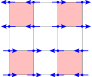
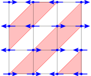
Figure 1: The two possible collinear configurations for the $J_{1}-J_{2}-J_{3}$ model: (a) orthogonal double stripe (ODS) and (b) diagonal double stripe (DDS).

There is one family of FeSCs - 11 Fe-chalcogenides Fe_1+yTe_1-xSe_x, in which smooth evolution between parent and optimally doped compounds does not hold. Magnetism in these materials changes considerably between $x=0$ and $x\sim 0.5$, where the $T_{c}$ is the largest. Near optimal doping magnetic fluctuations are peaked at or near $(0,\pi)$ and $(\pi,0)$, as in Fe-pnictides, while magnetic order in a parent compound Fe_1+yTe has very different momenta $\pm(\pi/2,\pm\pi/2)$ Li09 ; Liu10 ; Lipscombe11 ; Zaliznyak11 ; Zaliznyak12 . Upon doping, the spectral weight at $\pm(\pi/2,\pm\pi/2)$ decreases, and the spectral weight at $(0,\pi)$ and $(\pi,0)$ increases Liu10 . The transport properties of Fe_1+yTe are also quite different from those of parent compounds of Fe-pnictides: the resistivity, $\rho(T)$, of Fe_1+yTe does not show a prominent increase with increasing $T$, but instead remains flat and even shows a small increase as $T$ decreases Mizuguchi10 . ARPES studies of Fe_1+yTe show that low-energy spectra are very broad Xia09 , consistent with the notion that electrons are not propagating. These observations lead several groups to suggest that parent Fe-chalcogenides are more correlated than parent Fe-pnictides, and magnetism in Fe_1+yTe can be understood by assuming that electrons are ”almost” localized and interact magnetically via a Heisenberg exchange Subedi08 ; Ma09 ; Yu11 ; Hu12 . This scenario is in line with a more generic idea Si08 ; Zhao08 ; Yao2008 that in any FeSc, a certain percentage of electronic states are localized and phase separated from itinerant electrons, and the percentage of localized states varies between different materials. An alternative scenario for FeTe, which we don’t discuss here, is orbital order orbital

In this communication we apply the localized electron scenario to Fe_1+yTe and verify whether the observed commensurate $\pm(\pi/2,\pm\pi/2)$ order can be obtained in a Heisenberg model with exchange interactions up to third neighbors. Classically, $\pm(\pi/2,\pm\pi/2)$ order is unstable with respect to a spiral order for any non-zero first neighbor exchange, unless one artificially breaks $C_{4}$ symmetry and sets interactions to be spatially anisotropic Zhao08 ; Lipscombe11 . We analyze the isotropic quantum Heisenberg model and show that quantum fluctuations do stabilize a commensurate $\pm(\pi/2,\pm\pi/2)$ order in some range of parameters. However, this stabilization does not uniquely determine spin configuration as a generic $\pm(\pi/2,\pm\pi/2)$ order is a superposition of two different $Q-$vectors: ${\bf Q}_{1}=(\pi/2,-\pi/2)$, and ${\bf Q}_{2}=(\pi/2,\pi/2)$: ${\bf S}({\bf r})={\bf\Delta}_{1}\cos{{\bf Q}_{1}{\bf r}}+{\bf\Delta}^{{}^{\prime}}_{1}\sin{{\bf Q}_{1}{\bf r}}+{\bf\Delta}_{2}\cos{{\bf Q}_{2}{\bf r}}+{\bf\Delta}^{{}^{\prime}}_{2}\sin{{\bf Q}_{2}{\bf r}}$, with $|{\bf\Delta}_{i}|=|{\bf\Delta}^{{}^{\prime}}_{i}|=\Delta$ and ${\bf\Delta}_{1}\cdot{\bf\Delta}_{2}={\bf\Delta}^{{}^{\prime}}_{1}\cdot{\bf\Delta}^{{}^{\prime}}_{2}=0$. In Fig. 1 we show two prototypical commensurate spin configurations – a single $Q$ bi-collinear spin order (${\bf\Delta}_{1}={\bf\Delta}^{{}^{\prime}}_{1}={\bf\Delta}$, ${\bf\Delta}_{2}={\bf\Delta}^{{}^{\prime}}_{2}=0$), which breaks $C_{4}$, and a double $Q$ plaquette order (${\bf\Delta}^{{}^{\prime}}_{1}={\bf\Delta}_{2}={\bf\Delta}$, ${\bf\Delta}_{1}={\bf\Delta}^{{}^{\prime}}_{2}=0$), which preserves $C_{4}$ symmetry, but breaks $Z_{4}$ translational symmetry (four equivalent plaquette states are obtained by moving a black square in Fig. 1a by one lattice site in either $x$ or $y$ direction). Bi-collinear spin order is often called diagonal double stripe (DDS), and plaquette order is called orthogonal double stripe (ODS), and we use these notations below. The real-space configuration for both orders is ”up-up-down-down” along $x$ and $y$ directions.

Most of previous theoretical and experimental works assumed that the commensurate order is DDS Johnston10 and studied in detail the feedback from this order on electrons Lipscombe11 . We argue that quantum fluctuations of spins actually select ODS order as a stable collinear state for weak but finite nearest-neighbor exchange $J_{1}$, while DDS state is unstable for any non-zero $J_{1}$. The DDS and the ODS orders have qualitatively different forms of the static structure factor $S(q)$ (two peaks vs four peaks), but this is difficult to detect in real materials because of domains. The authors of Zaliznyak11 however argued that form of $S(q)$ in a paramagnetic phase allows one to distinguish between DDS and ODS, even in the presence of domains, and found that their results are consistent with strong ODS fluctuations. Another argument in favor of the $C_{4}$ preserving ODS spin order is the absence of orthogonal distortion in Fe_1+yTe – there is a monoclinic distortion below $T_{N}$, but this does not break rotational in-plane $C_{4}$ symmetry. There is also numerical evidence – ODS order has been found in exact diagonalization studies of $J_{1}-J_{2}-J_{3}$ model on clusters up to 36 spins Sindzingre09 . The same ODS order has been found in the mean-field studies of the $t-J$ model in another Fe-chalcogenide K_0.8Fe_1.6Se₂ graf .

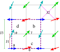
Figure 2: Spin order in the classical $J_{1}-J_{2}-J_{3}$ model at $J_{1}=0$. Classically degenerate configurations form four sublattices, labeled as $a,b,c$, and $d$. A configuration with arbitrary $\gamma$, $\theta$, and $\phi$ is a ground state. In our notations, sublattice spins are ${\bf\Delta}_{1}+{\bf\Delta}_{2}$, ${\bf\Delta}_{1}-{\bf\Delta}_{2}$, ${\bf\Delta}^{{}^{\prime}}_{1}-{\bf\Delta}^{{}^{\prime}}_{2}$, and ${\bf\Delta}^{{}^{\prime}}_{1}+{\bf\Delta}^{{}^{\prime}}_{2}$, respectively.

Model. We follow earlier works and model magnetic interactions in Fe_1+yTe by a $J_{1}-J_{2}-J_{3}$ Heisenberg model  Ma09 ; Sindzingre09 ; Reuter11 ; Yu11 :

$$H=\sum_{n=1}^{3}J_{n}\sum_{\langle ij\rangle}\vec{S}_{i}\cdot\vec{S}_{i+n}$$ (1)

where $J_{1},J_{2}$, and $J_{3}$ are antiferromagnetic exchange couplings between first-, second-, and third-nearest neighbors. For Fe_1+yTe the values of $J_{1},J_{2}$, and $J_{3}$ have been estimated in Ma09 and found to be in the range $J_{3}>\frac{J_{2}}{2}\gg J_{1}$. In this limit, the classical ground state of (1) is a spiral with the pitch vector $\mathbf{Q}=(\pm q,\pm q)$, where $q=\arccos(\frac{-J_{1}}{2J_{2}+4J_{3}})$ Mambrini2006 . At $J_{1}=0$, the model has an extensive degeneracy, and any order with momentum $\pm(\pi/2,\pm\pi/2)$ is the classical ground state, including DDS, ODS, and an infinite number of other four-sublattice states (Fig. 2).

We consider here what happens in the quantum model, at a finite $J_{1}$. We show that the ODS state is unambiguously selected by quantum fluctuations to be the ground state in some range of $J_{1}$, before a spiral order sets in. Our key reasoning is that only some classically degenerate ground states at $J_{1}=0$ are degenerate by symmetry; others are ”accidentally degenerate”. The situation is quite similar to the one in the well-known $J_{1}-J_{2}$ model at $J_{2}>J_{1}/2$ J1J2 . We argue that quantum fluctuations lift accidental degeneracies and gap out some of the spin-wave modes which in the classical limit become unstable (imaginary) at $J_{1}\neq 0$. For the DDS state the lifting of the accidental degeneracies does not help, as the modes which become unstable at a finite $J_{1}$ are the true Goldstone modes at $J_{1}=0$. On the other hand, for ODS state classically unstable modes are accidental zero modes at $J_{1}=0$, and quantum fluctuations lift the energies of these modes to finite values, making ODS the state stable in a finite range of $J_{1}$. We verified that ODS state is indeed the ground state in this range.

Large-S spin-wave calculations. We consider large value of spin $S$ and study the role of quantum fluctuations within $1/S$ expansion. The computational steps are presented in suppl . For $J_{1}=0$, spins on even and odd sites form two non-interacting sublattices, each described by $J_{2}-J_{3}$ model. This model is identical to $"J_{1}-J_{2}"$ model, with diagonal hopping $J_{2}$ playing the role of $"J_{1}"$ and third-neighbor hopping $J_{3}$ playing the role of $"J_{2}"$. One can use this analogy and borrow the results of the quantum analysis of $"J_{1}-J_{2}"$ model J1J2 . For $J_{3}>J_{2}/2$ (which holds in Fe_1+yTe), quantum fluctuations select stripe configurations within each sublattice, i.e. the angle $\gamma$ in Fig.2 is locked at $\gamma=0$ or $\gamma=\pi$, and the angle $\theta$ is locked at $\theta=\phi$ or $\theta=\pi+\phi$. The states with $\gamma=0$ and $\gamma=\pi$ are equivalent up to an interchange of $X$ and $Y$ directions, and below we set $\gamma=0$. The collinear DDS and ODS states belong to the manifold of selected states and correspond to different locking of the angle $\phi$ between the nearest-neighbor spins: DDS state corresponds to $\phi=0,\theta=\pi$ or $\phi=\pi,\theta=0$, while ODS corresponds to $\phi=\theta=0$ or $\phi=\theta=\pi$.

To analyze whether a generic state selected by quantum fluctuations at $J_{1}=0$ remains stable at a finite value of $J_{1}$, we need to know its excitation spectrum. At $J_{1}=0$, spins on even and odd sites are decoupled, each sublattice is described by its own bose field ($\alpha_{\mathbf{k}}$ for even sites and $\beta_{\mathbf{k}}$ for odd sites), and spin-wave excitations are described by

$$H_{sw}=S(\Omega_{\alpha\mathbf{k}}\alpha^{\dagger}_{\mathbf{k}}\alpha_{\mathbf{k}}+\Omega_{\beta\mathbf{k}}\beta^{\dagger}_{\mathbf{k}}\beta_{\mathbf{k}}),$$ (2)

The classical spin-wave spectrum is the same for all selected states

$$\Omega_{\mathbf{k}}=S(A^{2}_{\mathbf{k}}-B^{2}_{\mathbf{k}})^{1/2},~{}A_{\mathbf{k}}=4J_{3}+2J_{2}\cos(k_{x}+k_{y}),$$

$$B_{\mathbf{k}}=2J_{2}(\cos 2k_{x}+\cos 2k_{y})+2J_{2}\cos(k_{x}-k_{y}).$$ (3)

This spectrum contains nodes at $\pm(\pi/2,\pm\pi/2)$, but some of them are not symmetry-related and are lifted by quantum fluctuations. For the sublattice made of even sites, the order has momentum $\pm(\pi/2,-\pi/2)$ (Fig. 2 b), hence the true nodes are located only at these momenta, while the ones at $\pm(\pi/2,\pi/2)$ must be lifted. For the sublattice made out of spins at odd sites, the order has momentum $\pm(\pi/2,\pi/2)$ if we take $\theta=\phi$, like in the ODS, and $\pm(\pi/2,-\pi/2)$ if we take $\theta=\pi+\phi$, like in the DDS. Quantum fluctuations then must lift the nodes at $\pm(\pi/2,-\pi/2)$ and at $\pm(\pi/2,\pi/2)$ for the ODS and the DDS state, respectively. We computed quantum corrections to the spectrum in Eq. (3) within perturbation theory to order $1/S$ and indeed found that accidental nodes are lifted by quantum fluctuations and only true Goldstone modes remain suppl .

We next set $J_{1}$ to be small but finite and consider which of stripe states, if any, remain stable. The qualitative reasoning is the following: a non-zero $J_{1}$ couples the two sublattices and adds to the Hamiltonian (2) the terms in the form $\alpha^{\dagger}_{\mathbf{k}}\beta_{\mathbf{k}}$ and $\alpha_{\mathbf{k}}\beta_{\mathbf{k}}$. For the DDS state (or, more accurately, for the DDS family of states as we keep $\phi$ as a parameter) the stripes on even and odd sites are directed parallel to each other, and the dispersions of $\alpha_{\mathbf{k}}$ and $\beta_{\mathbf{k}}$ fields are identical, including $O(1/S)$ terms. The two dispersions are then gapless at the same momenta $\mathbf{k}=\pm(\pi/2,-\pi/2)$. Around these $\mathbf{k}$ points, the perturbation theory in $J_{1}$ is singular, as there is no symmetry requirement which would force the coupling to vanish at $\pm(\pi/2,-\pi/2)$. As a result, the excitations become purely imaginary close enough to $\pm(\pi/2,-\pi/2)$, which implies that the DDS states are unstable at any non-zero $J_{1}$. On the other hand, for the ODS family of states, the dispersions $\Omega^{\alpha}_{\mathbf{k}}$ and $\Omega^{\beta}_{\mathbf{k}}$ have nodes at different momenta, $\pm(\pi/2,-\pi/2)$ and $\pm(\pi/2,\pi/2)$, respectively. Because of this disparity, perturbation theory near either $\pm(\pi/2,-\pi/2)$ or $\pm(\pi/2,\pi/2)$ is not singular, and corrections in $J_{1}$ only gradually shift the values of spin-wave velocities thus keeping ODS states stable.

We verified this reasoning by explicit calculations. We first obtained the $J_{1}$-induced interaction in terms of the original Holstein-Primakoff bosons and then re-expressed it in terms of $\alpha_{\mathbf{k}}$ and $\beta_{\mathbf{k}}$ bosons from Eq. (2), which are related to the original ones by Bogoliubov transformation. The $u_{\mathbf{k}}v_{\mathbf{k}}$-coefficients of this transformation dress up the interaction terms. For the DDS states, expanding the Hamltonian near the true Goldstone points at $(\pi/2,-\pi/2)$ as $\mathbf{k}=(\pi/2,-\pi/2)+\mathbf{\tilde{k}}$ we obtain $H_{DDS}=H_{sw}+\delta H_{DDS}$, where $H_{sw}$ is given by (2) with

$$\Omega^{\alpha}_{\mathbf{\tilde{k}}}=\Omega^{\beta}_{\mathbf{\tilde{k}}}\approx 4S\sqrt{J_{3}(2J_{3}+J_{2})}({\tilde{k}}^{2}_{x}+{\tilde{k}}^{2}_{y}-2a{\tilde{k}}_{x}{\tilde{k}}_{y})^{1/2},$$ (4)

where $a=\frac{J_{2}}{2J_{3}}<1$, and

$$\delta H_{DDS}=\Delta^{DDS}{\mathbf{\tilde{k}}}(\alpha_{\mathbf{\tilde{k}}}^{\dagger}\beta_{\mathbf{\tilde{k}}}+\alpha_{\mathbf{\tilde{k}}}\beta_{\mathbf{-{\tilde{k}}}}+h.c)$$ (5)

where

$$\Delta^{DDS}_{\mathbf{\tilde{k}}}=\frac{J_{1}S}{2}\left(\frac{2J_{3}+J_{2}}{J_{3}}\right)^{1/2}\frac{{\tilde{k}}_{y}-{\tilde{k}}_{x}}{({\tilde{k}}^{2}_{x}+{\tilde{k}}^{2}_{y}-2a{\tilde{k}}_{x}{\tilde{k}}_{y})^{1/2}}$$ (6)

The coupling term remains finite when ${\tilde{k}}_{x,y}$ tends to zero, except for special directions. Diagonalizing (5) we find that at low enough ${\tilde{k}}$ one of the two solutions is $E^{2}_{\tilde{k}}\approx-2\Omega^{\alpha(\beta)}_{\mathbf{\tilde{k}}}\Delta^{DDS}_{\mathbf{\tilde{k}}}$. A negative $E^{2}_{\tilde{k}}$ implies that fluctuations around a DDS state grow exponentially with time and make this family of states unstable.

For the ODS states the situation is different because near any of the points $\pm(\pi/2,-\pi/2)$ or $\pm(\pi/2,\pi/2)$, the zero in one of the spin-wave branches is lifted by quantum fluctuations. For example, near $(-\pi/2,\pi/2)$ expanding of the Hamiltonian again gives $H_{ODS}=H_{sw}+\delta H_{ODS}$, however now only $\Omega^{\alpha}_{\mathbf{\tilde{k}}}$ is gapless, while $\Omega^{\beta}_{\mathbf{\tilde{k}}}$ is gapped with the gap of the order $1/S$. The interaction term $\delta H_{ODS}$ has the same form as in (5), but with

$$\Delta^{ODS}_{{\mathbf{\tilde{k}}}}=2J_{1}S^{2}(2J_{3}+J_{2})\frac{{\tilde{k}}_{y}-{\tilde{k}}_{x}}{(\Omega^{\alpha}_{\tilde{k}}\Omega^{\beta}_{\tilde{k}})^{1/2}}=O\left(J_{1}S^{3/2}|{\tilde{k}}|^{1/2}\right).$$ (7)

Diagonalizing $H_{ODS}$ we find two solutions,

$$E^{2}_{1,2} = \frac{1}{2}\Bigl{(}(\Omega^{\alpha}_{\tilde{k}})^{2}+(\Omega^{\beta}_{\tilde{k}})^{2}$$

$$\pm\sqrt{((\Omega^{\alpha}_{\tilde{k}})^{2}-(\Omega^{\beta}_{\tilde{k}})^{2})^{2}+16(\Delta^{ODS}_{\mathbf{\tilde{k}}})^{2}\Omega^{\alpha}_{\tilde{k}}.\Omega^{\beta}_{\tilde{k}}}\Bigr{)}.$$

One of the solutions is gapped to order $1/S$, the other is linear in ${\tilde{k}}$ with a stiffness which differs from its value at $J_{1}=0$ by $O(J_{1}S/J_{3})$. We see that the ODS states are stable (for any $\phi$) as long as $J_{1}S/J_{3}$ is small.

On a more careful look, we find that the ODS spin order allows for $J_{1}-$induced umklapp processes, which also renormalize the dispersions of the ODS states. Indeed, because ODS state breaks $Z_{4}$ translational symmetry, the $J_{1}$ interaction contains not only the terms at zero transferred momentum, as in (5), but also terms with momentum transfer in multiples of $\pi$ along each axis. Near $k=(\pi/2,-\pi/2)$, the most relevant of such umklapp terms is the one with momentum ${\bar{Q}}=(0,\pi)$, which connects a gapless $\alpha_{\tilde{k}}$ boson at $(\pi/2,-\pi/2)$, and a gapless $\beta_{\tilde{k}}$ boson at $(\pi/2,\pi/2)$. However, because breaking of $Z_{4}$ is equivalent to breaking local inversion symmetry (a reflection around one column or one row in Fig. 1a), the umklapp vertices $\Delta^{U,ODS}_{\mathbf{\tilde{k}}}$ contain extra momentum gradient compared to non-umklapp vertices. In explicit form, we find at small ${\mathbf{\tilde{k}}}=\mathbf{k}-(\pi/2,-\pi/2)$,

$$\Delta^{U,ODS}_{\mathbf{\tilde{k}}}=-i\frac{J_{1}}{4}\left(\frac{\Omega^{\alpha}_{\tilde{k}}\Omega^{\beta}_{{\tilde{k}}+{\bar{Q}}}}{4J^{2}_{3}-J^{2}_{2}}\right)^{1/2}\cos\phi~{},$$ (9)

where $\Omega^{\alpha}_{\tilde{k}},\Omega^{\beta}_{\tilde{k}+{\bf Q}}=4S(J_{3}(2J_{3}\pm J_{2}))^{1/2}({\tilde{k}}^{2}_{x}+{\tilde{k}}^{2}_{y}\mp 2{\tilde{k}}_{x}{\tilde{k}}_{y})^{1/2}$ and the angle $\phi$ specifies the spin order within the ODS family of states. We see that $\Delta^{U,ODS}_{\mathbf{\tilde{k}}}$ scales linearly with ${\mathbf{\tilde{k}}}$, i.e., is of the same order as $\Omega^{\alpha\beta}_{\tilde{k}}$. We computed the corrections to spin-wave velocity and found that they scale as $J_{1}/\sqrt{4J^{2}_{3}-J^{2}_{1}}$, i.e., are small. At the same time, we see from the Eq.(9) that $\Delta^{U,ODS}_{\mathbf{\tilde{k}}}$ depends on the angle $\phi$. Respectively, the corrections to the ground state energy also depend on $\phi$ and should select which state within the ODS family has the lowest energy. The computation is straightforward and yields $\Delta E_{gr}=-A\cos^{2}\phi$, with $A>0$. We see that the collinear ODS state, for which $\phi=0$ or $\pi$, is indeed the state with the lowest energy.

The outcome of our analysis is that the collinear ODS state remains stable and has the lowest energy within a family of similar states. At small $J_{1}$, the ODS state has a finite stiffness towards fluctuations which tend to break collinear order in favor of a spiral one. The ODS state remains stable up to $J_{1}\sim J_{3}/S$, at larger $J_{1}$ the stiffness changes sign, and the system develops a spiral order.

Experimental signatures of ODS state. Because the ODS state does not break $C_{4}$ translational symmetry, it does not cause a pre-emptive spin-nematic order, in contrast to parent compounds of other FeSCs Fernandes12 . The data for Fe_1+yTe show that the system develops a monoclinic distortion below a certain $T$, but in-plane $C_{4}$ symmetry remains unbroken (it only breaks in doped compounds Fe_1+yTe_1-xSe_x with $x>0.5$  Mizuguchi10 ). The unbroken $C_{4}$ symmetry in the ordered state also manifests itself in the $C_{4}$ symmetry of the static structure factor $S(q)$ obtained in neutron scattering experiments  Zaliznyak11 . We computed $S(q)$ for both the DDS and the ODS states, and we indeed found that the structure factor for the ODS order has four identical peaks at $(\pm\pi/2,\pm\pi/2)$, while the structure factor for the DDS state has only two peaks at $(\pi/2,-\pi/2)$ and $(-\pi/2,\pi/2)$. While the observed four peaks are consistent with ODS, we caution that the absence of the anisotropy in the structure factor obtained in neutron scattering could be due to the twinning of the crystal. However, as the magnetic domain’s structure of the crystal can be controlled using polarized neutrons, the careful analysis of the neutron scattering data might dissect the contribution from different domains. The authors of Ref. Zaliznyak11 made another argument that, even in a twinned crystal, the form of $S(q)$ throughout the Brillouin zone differentiates between strong DDS and ODS fluctuations, and argued that their data are more consistent with tendency towards ODS order. This again agrees with our results.

Summary. In this communication we analyzed the type of magnetic order in Fe_1+yTe – the parent compound in a family of Fe-chalcogenide superconductors. The magnetic order in this material is different from in other parent compounds of FeSCs – spins are ordered in up-up-down-down fashion (Fig. 2). Experiments show Mizuguchi10 ; Tamai10 that the tendency towards Mott physics is stronger in Fe_1+yTe than in other parent compounds of FeSCs, suggesting that the magnetic order in Fe_1+yTe can be reasonably well understood within the localized scenario by solving the Heisenberg model with exchange interaction extending up to third neighbors Ma09 . Several groups argued Ma09 ; Li09 ; Lipscombe11 ; Fang12 that the ordered up-up-down-down spin configuration is diagonal double stripe. Such an order breaks $C_{4}$ lattice rotational symmetry. We argued, based on our analysis of quantum fluctuations in the Heisenberg model with first, second, and third-neighbor exchange, that such a state is unstable, but another up-up-down-down state – the orthogonal double stripe, is stable and is the ground state in some parameter range. This state (which is also called a plaquette state) breaks $Z_{4}$ translational symmetry, preserves $C_{4}$ symmetry, and does not cause orthorhombic distortion. Also, its structure factor has four equivalent peaks at $(\pm\pi/2,\pm\pi/2)$, in agreement with recent neutron scattering studies of Fe_1+yTe Zaliznyak11 . An interesting issue that deserves further study is whether $Z_{4}$ translational symmetry can be broken before a true ODS spin order sets in, as it happens in other systems chern .

Acknowledgement. We acknowledge useful conversations with C. Batista, R. Fernandes, G-W. Chern, M. Graf, B. Lake, A. Nevidomskyy, J. Schmalian, N. Shannon, and I Zaliznyak. N.B.P. is supported by NSF-DMR-0844115, A.V.C. is supported by NSF-DMR-0906953.

In this Supplementary Material we provide details of our analysis of how quantum fluctuations lift accidental nodes in the spin-wave spectra of the sub-set of states selected by quantum fluctuations in the $J_{1}-J_{2}-J_{3}$ model at $J_{3}>J_{2}/2$ and $J_{1}=0$ (i.e., in the $J_{2}-J_{3}$ model with $J_{3}>J_{2}/2$). The Hamiltonian for the model is given by Eq. (1) in the main text. At $J_{1}=0$ spins on even and odd sites do not interact with each other. It is therefore sufficient to consider only the sub-set made out of spins on, say, even sites.

Classically degenerate ground states are shown in Fig. 2 of the main text. For spins on even sites, any two-sublattice configuration with arbitrary angle $\gamma$ between spins in $a$ and $b$ sublattices is the ground state. Like we said in the text, quantum fluctuations break this degeneracy and select the states at $\gamma=0$ or $\gamma=\pi$ as the only two ground states. The state with $\gamma=0$ can be viewed as a spiral state with $Q_{1}=(\pi/2,-\pi/2)$, and the $\gamma=\pi$ state corresponds to a spiral with $Q_{2}=(\pi/2,\pi/2)$. Because only even cites are involved, configurations with $Q_{i}$ and $-Q_{i}$ are identical.

The classical spectrum of either $Q_{1}$ or $Q_{2}$ state contains zero modes at corresponding $Q$, which must be there by Goldstone theorem, but also contains zero modes at ”wrong Q” (at $Q_{2}$ for the $Q_{1}$ spiral and vise versa). These last modes are not associated with symmetry breaking (i.e., are ”accidental”) and must be lifted by quantum fluctuations. In the main text we stated that quantum fluctuations do gap accidental zero modes and studied the consequences. Here we show how this actually happens. For definiteness, we consider $Q_{1}$ configuration ($\gamma=0$).

The lifting of accidental zero modes can be studied within the original two-sublattice picture, with two different bosons describing fluctuations of spins in $a$ and $b$ sublattices. It is more convenient, however, to perform a uniform rotation to a local reference frame in which the magnetic order is ferromagnetic and describe the excitation spectrum using just one Holstein-Primakoff bose operator $a_{i}$:

$$\begin{array}[]{l}S^{z}_{i}=S-a^{\dagger}_{i}a_{i}\\ S^{+}_{i}=(2S-a^{\dagger}_{i}a_{i})^{\frac{1}{2}}a_{i}~{}~{}~{}~{}~{}~{}~{}~{}~{}~{}(S.1)\\ S^{-}_{i}=a^{\dagger}_{i}(2S-a^{\dagger}_{i}a_{i})^{\frac{1}{2}}~{},\end{array}$$ (13)

As it is customary to spin-wave analysis, we assume that $S$ is large. Our goal is to obtain the excitation spectrum for $Q_{1}$ configuration including terms of order $1/S$, which describe quantum fluctuations. Accordingly, we substitute Eq. (S.1) into Hamiltonian (Eq. (1)) and then expand it to the quartic order in $a$ field. We obtain

$$H=E_{0}+S(H_{2}+H_{4})~{},~{}~{}~{}~{}~{}~{}~{}(S.2)$$

where $H_{2}$ and $H_{4}$ are the quadratic and the quartic terms, respectively. In momentum space, we have

$$H_{2}= \sum_{\mathbf{k}}\Bigl{(}A_{\mathbf{k}}a^{\dagger}_{\mathbf{k}}a_{\mathbf{k}}+\frac{B_{\mathbf{k}}}{2}(a_{\mathbf{k}}a_{\mathbf{-k}}+h.c.)\Bigr{)},~{}~{}(S.3)$$

where

$$A_{\mathbf{k}} = 4J_{3}+2J_{2}\cos(k_{x}+k_{y})~{}~{}~{}~{}~{}~{}~{}~{}~{}~{}~{}~{}~{}~{}~{}(S.4)$$

$$B_{\mathbf{k}} = -2J_{3}(\cos(2k_{x})+\cos(2k_{y}))-2J_{2}\cos(k_{x}-k_{y})$$

and ${\bf k}$ is defined in the first magnetic BZ. The quartic part of the large-S expansion is given by

$$H_{4}=\frac{J_{2}}{8NS}\sum_{\{\mathbf{k}_{i}\}}\delta\Bigl{(}\sum_{i}\mathbf{k}_{i}\Bigr{)}\Bigl{[}a^{\dagger}_{-{\mathbf{k}}_{1}}a_{{\mathbf{k}}_{2}}a_{{\mathbf{k}}_{3}}a_{{\mathbf{k}}_{4}}\cos(k_{4x}-k_{4y})$$

$$-a^{\dagger}_{-{\mathbf{k}}_{1}}a^{\dagger}_{-{\mathbf{k}}_{2}}a_{{\mathbf{k}}_{3}}a_{{\mathbf{k}}_{4}}\cos(k_{4x}+k_{4y})~{}~{}~{}~{}~{}~{}~{}~{}~{}~{}~{}~{}~{}~{}~{}~{}(S.5)$$

$$-2a^{\dagger}_{-{\mathbf{k}}_{1}}a^{\dagger}_{-{\mathbf{k}}_{2}}a_{{\mathbf{k}}_{3}}a_{{\mathbf{k}}_{4}}\sin(k_{2x}+k_{4x})\sin(k_{2y}+k_{4y})+h.c.\Bigr{]}$$

$$+\frac{J_{3}}{8NS}\sum_{\{\mathbf{k}_{i}\}}\delta\Bigl{(}\sum_{i}\mathbf{k}_{i}\Bigr{)}\Bigl{[}a^{\dagger}_{-{\mathbf{k}}_{1}}a_{{\mathbf{k}}_{2}}a_{{\mathbf{k}}_{3}}a_{{\mathbf{k}}_{4}}(\cos 2k_{4x}+\cos 2k_{4y})$$

$$-a^{\dagger}_{-{\mathbf{k}}_{1}}a^{\dagger}_{-{\mathbf{k}}_{2}}a_{{\mathbf{k}}_{3}}a_{{\mathbf{k}}_{4}}(\cos 2(k_{2y}+k_{4y})+\cos 2(k_{2x}+k_{4x}))+h.c.\Bigr{]}$$

The quadratic Hamiltonian $H_{2}$ is diagonalized by introducing the Bogoliubov transformation, $\alpha_{\mathbf{k}}=u_{\mathbf{k}}a_{\mathbf{k}}-v_{\mathbf{k}}a^{\dagger}_{\mathbf{-k}}$, where the coherence factors $u_{\mathbf{k}}$ and $v_{\mathbf{k}}$ are determined by

$$u_{\mathbf{k}} = \frac{1}{2}\sqrt{\frac{A_{\mathbf{k}}+\Omega_{\mathbf{k}}}{\Omega_{\mathbf{k}}}}~{},$$

$$v_{\mathbf{k}} = -\frac{\text{sign}B_{\mathbf{k}}}{2}\sqrt{\frac{A_{\mathbf{k}}-\Omega_{\mathbf{k}}}{\Omega_{\mathbf{k}}}}$$

and

$$\Omega_{\mathbf{k}}=S\sqrt{A_{\mathbf{k}}^{2}-B_{\mathbf{k}}^{2}}~{}.$$

The diagonalized Hamiltonian $H_{2}$ is given by

$$H_{2}=E_{2}+\sum_{\mathbf{k}}\Omega_{\mathbf{k}}\alpha^{\dagger}_{\mathbf{k}}\alpha_{\mathbf{k}}~{},~{}~{}~{}~{}~{}~{}~{}~{}(S.6)$$

where

$$E_{2}=\frac{S}{2}\sum_{\mathbf{k}}(-A_{\mathbf{k}}+\Omega_{\mathbf{k}})~{}~{}~{}~{}~{}~{}~{}~{}~{}~{}~{}~{}(S.7)$$

is the contribution to the ground state energy from non-interacting $a$-bosons

The spin-wave dispersion of non-interacting bosons is $\Omega_{\mathbf{k}}$. At $\mathbf{k}=\pm Q_{1}$ and $\mathbf{k}=\pm Q_{2}$, $A_{Q_{1(2)}}=B_{Q_{1(2)}}=4J_{3}\pm 2J_{2}$, where + and - signs are for $Q_{1}$ and $Q_{2}$, respectively. As a result, $\Omega_{Q_{1}}=\Omega_{Q_{2}}=0$. However, as we said, only the zero mode at $\mathbf{k}=\pm Q_{1}$ is the true Goldstone mode, the other one is accidental and must be gapped by quantum fluctuations. To show this, we have to compute 1/S corrections to the spectrum at these points.

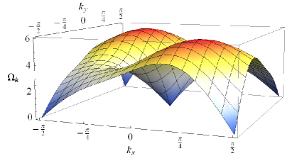
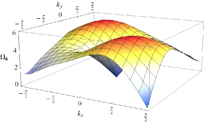
Figure 3: Excitation spectrum for $Q_{1}$ spiral. Top panel: The spectrum of non-interacting bosons, Eq.(S.6) This spectrum contains zero modes at $\pm(\pi/2,\pi/2)$ and $\pm(\pi/2,-\pi/2)$ Bottom panel: the spectrum renormalized by quantum fluctuations to order $1/S$. The true Goldstone modes at $\pm\mathbf{Q_{1}}=\pm(\frac{\pi}{2},-\frac{\pi}{2})$ remain, but the accidental zeroes at $\pm\mathbf{Q}_{2}=\pm(\frac{\pi}{2},\frac{\pi}{2})$ are removed by quantum fluctuations.

The $1/S$ contribution to $\Omega_{\mathbf{k}}$ is obtained by evaluating the first-order correction from $H_{4}$ what amounts to decoupling of $H_{4}$ into the product of two pairs of $a-$ bosons and replacing one pair by its average value for non-interacting bosons. We first define the averages

$$K_{{\mathbf{q}}} = \langle a_{\mathbf{q}}^{\dagger}a_{\mathbf{q}}\rangle=v_{\mathbf{q}}^{2}~{},~{}~{}~{}~{}~{}~{}(S.8)$$

$$L_{{\mathbf{q}}} = \langle a_{\mathbf{q}}a_{-{\mathbf{q}}}\rangle=\langle a_{-\mathbf{q}}^{\dagger}a_{{\mathbf{q}}}^{\dagger}\rangle=u_{\mathbf{q}}v_{\mathbf{q}}~{}.$$

The decoupled $H_{4}$ is

$${\bar{H}}_{4} = \frac{1}{8NS}\sum_{\mathbf{k},q}\Bigl{(}a^{\dagger}_{\mathbf{k}}a_{\mathbf{k}}F_{1}({\mathbf{k}},{\mathbf{q}})+$$

$$(a_{\mathbf{k}}a_{-{\mathbf{k}}}+a_{-\mathbf{k}}^{\dagger}a_{{\mathbf{k}}}^{\dagger})\frac{F_{2}({\mathbf{k}},{\mathbf{q}})}{2}\Bigr{)},~{}(S.9)$$

where

$$F_{1}({\mathbf{k}},{\mathbf{q}})=-2J_{3}\Bigl{(}4K_{{\mathbf{q}}}(\cos^{2}(k_{x}-q_{x})+\cos^{2}(k_{y}-q_{y}))$$

$$-L_{{\mathbf{q}}}(2(\cos 2q_{x}+\cos 2q_{y})+\cos 2k_{x}+\cos 2k_{y})\Bigr{)}$$

$$-2J_{2}\Bigl{(}K_{{\mathbf{q}}}(4\sin(k_{x}-q_{x})\sin(k_{y}-q_{y})$$

$$+2\cos(k_{x}+k_{y})+2\cos(q_{x}+q_{y}))$$

$$-L_{{\mathbf{q}}}(2\cos(q_{x}-q_{y})+\cos(k_{x}-k_{y}))\Bigr{)},$$

$$F_{2}({\mathbf{k}},{\mathbf{q}})=2J_{3}\Bigl{(}K_{\mathbf{q}}(\cos 2q_{x}+\cos 2q_{y}$$

$$+2(\cos 2k_{x}+\cos 2k_{y}))$$

$$-2L_{\mathbf{q}}(\cos 2(k_{x}-q_{x})+\cos 2(k_{y}-q_{y}))\Bigr{)}$$

$$+2J_{2}\Bigl{(}K_{{\mathbf{q}}}(\cos(q_{x}-q_{y})+2\cos(k_{x}-k_{y}))$$

$$+L_{\mathbf{q}}(-4\sin(k_{x}-q_{x})\sin(k_{y}-q_{y})$$

$$-\cos(k_{x}+k_{y})-\cos(q_{x}+q_{y}))\Bigr{)}$$

Combining the decoupled $H_{4}$ with $H_{2}$ expressed in terms of original $a$-operators we obtain

$$H_{2}+{\bar{H}}_{4}=\sum_{\mathbf{k}}\Bigl{[}(A_{\mathbf{k}}+\frac{A^{(4)}_{\mathbf{k}}}{S})a^{\dagger}_{\mathbf{k}}a_{\mathbf{k}}+$$

$$\frac{1}{2}(B_{\mathbf{k}}+\frac{B^{(4)}_{\mathbf{k}}}{S})(a_{\mathbf{k}}a_{\mathbf{-k}}+h.c.)\Bigr{]},~{}~{}~{}~{}(S.10)$$

where

$$A^{(4)}_{\mathbf{k}} = \frac{1}{8N}\sum_{\mathbf{q}}F_{1}({\mathbf{k}},{\mathbf{q}}),$$

$$B^{(4)}_{\mathbf{k}} = \frac{1}{8N}\sum_{\mathbf{q}}F_{2}({\mathbf{k}},{\mathbf{q}})$$

At $\mathbf{k}=Q_{1}$ and $\mathbf{k}=Q_{2}$ we have

$$A^{(4)}_{\mathbf{Q_{1(2)}}} = \frac{-1}{4N}\sum_{\mathbf{q}}J_{3}\Bigl{(}4K_{{\mathbf{q}}}(\sin^{2}(q_{x})+\sin^{2}(q_{y}))$$

$$-L_{{\mathbf{q}}}(2(\cos 2q_{x}+\cos 2q_{y})-2)\Bigr{)}$$

$$+J_{2}\Bigl{(}K_{{\mathbf{q}}}(\mp 4\cos(q_{x})\cos(q_{y})$$

$$\pm 2+2\cos(q_{x}+q_{y}))$$

$$-L_{{\mathbf{q}}}(2\cos(q_{x}-q_{y})\mp 2)\Bigr{)},$$

$$B^{(4)}_{\mathbf{Q_{1(2)}}} = \frac{1}{4N}\sum_{\mathbf{q}}J_{3}\Bigl{(}K_{\mathbf{q}}(\cos 2q_{x}+\cos 2q_{y}-4)$$

$$+2L_{\mathbf{q}}(\cos 2q_{x}+\cos 2q_{y})\Bigr{)}$$

$$+J_{2}\Bigl{(}K_{{\mathbf{q}}}(\cos(q_{x}-q_{y})\mp 2)$$

$$+L_{\mathbf{q}}(\pm 4\cos(q_{x})\cos(q_{y})$$

$$\mp 1-\cos(q_{x}+q_{y}))\Bigr{)}~{},$$

where the upper and the lower signs correspond to $\mathbf{Q_{1}}$ and $\mathbf{Q_{2}}$ vectors, respectively. One can easily make sure that $A^{(4)}_{\mathbf{Q_{1}}}=B^{(4)}_{\mathbf{Q_{1}}}$, but $A^{(4)}_{\mathbf{Q_{2}}}\neq B^{(4)}_{\mathbf{Q_{2}}}$. Thus, when 1/S corrections are included, the spectrum at $\mathbf{Q_{1}}$ remains gapless, as it should be, but at $\mathbf{Q_{2}}$ the gap opens up, i.e., quantum fluctuations lift the accidental degeneracy at the ”wrong $Q$”. We computed the renormalized spectrum for all ${\mathbf{k}}$ and show the results in Fig.3. The renormalized spectrum, shown in the bottom panel, clearly has a gap at $\pm(\pi/2,\pi/2)$, where the spectrum of non-interacting bosons (top panel) has zero modes. We verified that the same effect (lifting of accidental nodes) holds if we use biquadratic spin interaction instead of quantum fluctuations.

Supplemental Material for Magnetism in parent Fe-chalcogenides: quantum fluctuations select a plaquette order Samuel Ducatman, Natalia B. Perkins, Andrey Chubukov

In this Supplementary Material we provide details of our analysis of how quantum fluctuations lift accidental nodes in the spin-wave spectra of the sub-set of states selected by quantum fluctuations in the $J_{1}-J_{2}-J_{3}$ model at $J_{3}>J_{2}/2$ and $J_{1}=0$ (i.e., in the $J_{2}-J_{3}$ model with $J_{3}>J_{2}/2$). The Hamiltonian for the model is given by Eq. (1) in the main text. At $J_{1}=0$ spins on even and odd sites do not interact with each other. It is therefore sufficient to consider only the sub-set made out of spins on, say, even sites.

Classically degenerate ground states are shown in Fig. 2 of the main text. For spins on even sites, any two-sublattice configuration with arbitrary angle $\gamma$ between spins in $a$ and $b$ sublattices is the ground state. Like we said in the text, quantum fluctuations break this degeneracy and select the states at $\gamma=0$ or $\gamma=\pi$ as the only two ground states. The state with $\gamma=0$ can be viewed as a stripe state with $Q_{1}=(\pi/2,-\pi/2)$, and the $\gamma=\pi$ state corresponds to a stripe with $Q_{2}=(\pi/2,\pi/2)$. Because only even cites are involved, configurations with $Q_{i}$ and $-Q_{i}$ are identical.

The classical spectrum of either $Q_{1}$ or $Q_{2}$ state contains zero modes at corresponding $Q$, which must be there by Goldstone theorem, but also contains zero modes at the ”wrong Q” (at $Q_{2}$ for the $Q_{1}$ stripe and vise versa). These last modes are not associated with symmetry breaking (i.e., are ”accidental”) and must be lifted by quantum fluctuations. We argued in the main text that quantum fluctuations as well as biquadratic exchange coupling gap accidental zero modes, and studied the consequences. Here we show how this actually happens in the quantum case. For definiteness, we consider $Q_{1}$ configuration ($\gamma=0$).

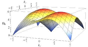
Figure 4: Excitation spectrum for $Q_{1}$ stripe. Top panel: The classical spectrum of $J_{2}-J_{3}$ model computed for $J_{2}=J_{3}=1$. This spectrum contains zero modes at $\pm(\pi/2,\pi/2)$ and $\pm(\pi/2,-\pi/2)$. Bottom panel: the spectrum for $J_{2}-J_{3}$ model in the presence of biquadratic exchange coupling $K=0.05$. The true Goldstone modes at $\pm\mathbf{Q_{1}}=\pm(\frac{\pi}{2},-\frac{\pi}{2})$ remain, but the accidental zeroes at $\pm\mathbf{Q}_{2}=\pm(\frac{\pi}{2},\frac{\pi}{2})$ are removed.

The lifting of accidental zero modes can be studied within the original two-sublattice picture, with two different bosons describing fluctuations of spins in $a$ and $b$ sublattices. It is more convenient, however, to perform a uniform rotation to a local reference frame in which the magnetic order is ferromagnetic, and describe the excitations using one Holstein-Primakoff bose operator $a_{i}$:

$$\begin{array}[]{l}S^{z}_{i}=S-a^{\dagger}_{i}a_{i}\\ S^{+}_{i}=(2S-a^{\dagger}_{i}a_{i})^{\frac{1}{2}}a_{i}~{}~{}~{}~{}~{}~{}~{}~{}~{}~{}(S.1)\\ S^{-}_{i}=a^{\dagger}_{i}(2S-a^{\dagger}_{i}a_{i})^{\frac{1}{2}}~{},\end{array}$$ (17)

As it is customary to spin-wave analysis, we assume that $S$ is large. Our goal is to obtain the excitation spectrum for $Q_{1}$ configuration including terms of order $1/S$, which describe quantum fluctuations. To get this spectrum, we substitute Eq. (S.1) into Hamiltonian (Eq. (1)) and expand it to the quartic order in $a$ field. We obtain

$$H=E_{0}+S(H_{2}+H_{4})~{},~{}~{}~{}~{}~{}~{}~{}(S.2)$$

where $H_{2}$ and $H_{4}$ are the quadratic and the quartic terms, respectively. In momentum space, we have

$$H_{2}= \sum_{\mathbf{k}}\Bigl{(}A_{\mathbf{k}}a^{\dagger}_{\mathbf{k}}a_{\mathbf{k}}+\frac{B_{\mathbf{k}}}{2}(a_{\mathbf{k}}a_{\mathbf{-k}}+h.c.)\Bigr{)},~{}~{}(S.3)$$

where

$$A_{\mathbf{k}} = 4J_{3}+2J_{2}\cos(k_{x}+k_{y})~{}~{}~{}~{}~{}~{}~{}~{}~{}~{}~{}~{}~{}~{}~{}(S.4)$$

$$B_{\mathbf{k}} = -2J_{3}(\cos(2k_{x})+\cos(2k_{y}))-2J_{2}\cos(k_{x}-k_{y})$$

and ${\bf k}$ is defined in the first magnetic BZ.

The quadratic Hamiltonian $H_{2}$ is diagonalized by the Bogoliubov transformation, $\alpha_{\mathbf{k}}=u_{\mathbf{k}}a_{\mathbf{k}}-v_{\mathbf{k}}a^{\dagger}_{\mathbf{-k}}$, where the factors $u_{\mathbf{k}}$ and $v_{\mathbf{k}}$ are determined by

$$u_{\mathbf{k}} = \sqrt{\frac{A_{\mathbf{k}}+\Omega_{\mathbf{k}}}{2\Omega_{\mathbf{k}}}}~{},$$

$$v_{\mathbf{k}} = -\text{sign}B_{\mathbf{k}}\sqrt{\frac{A_{\mathbf{k}}-\Omega_{\mathbf{k}}}{2\Omega_{\mathbf{k}}}}$$

and

$$\Omega_{\mathbf{k}}=S\sqrt{A_{\mathbf{k}}^{2}-B_{\mathbf{k}}^{2}}~{}.$$ (18)

The diagonalized Hamiltonian $H_{2}$ is given by

$$H_{2}=E_{2}+\sum_{\mathbf{k}}\Omega_{\mathbf{k}}\alpha^{\dagger}_{\mathbf{k}}\alpha_{\mathbf{k}}~{},~{}~{}~{}~{}~{}~{}~{}~{}(S.5)$$

where

$$E_{2}=\frac{S}{2}\sum_{\mathbf{k}}(-A_{\mathbf{k}}+\Omega_{\mathbf{k}})~{}~{}~{}~{}~{}~{}~{}~{}~{}~{}~{}~{}(S.6)$$

is the contribution to the ground state energy from non-interacting bosons

Eq. (18) gives spin-wave dispersion without $1/S$ corrections. At $\mathbf{k}=\pm Q_{1}$ and $\mathbf{k}=\pm Q_{2}$, $A_{Q_{1(2)}}=B_{Q_{1(2)}}=4J_{3}\pm 2J_{2}$, where + and - signs are for $Q_{1}$ and $Q_{2}$, respectively. As a result, $\Omega_{Q_{1}}=\Omega_{Q_{2}}=0$. However, only the zero mode at $\mathbf{k}=\pm Q_{1}$ is the true Goldstone mode, the other one is accidental and must be lifted by quantum fluctuations. To show this, we compute 1/S corrections to the spectrum at these points.

The quartic term in the Hamiltonian is given by

$$H_{4}=\frac{1}{2S}\sum_{ij}J_{ij}\Bigl{(}\cos\phi_{ij}a^{\dagger}_{i}a_{i}a^{\dagger}_{j}a_{j}+~{}~{}~{}~{}~{}~{}(S.7)$$

$$\frac{1-\cos\phi_{ij}}{8}\bigl{(}a_{i}a^{\dagger}_{j}a_{j}a_{j}+a^{\dagger}_{i}a_{i}a_{i}a_{j}+a^{\dagger}_{i}a^{\dagger}_{j}a^{\dagger}_{j}a_{j}+a^{\dagger}_{i}a^{\dagger}_{i}a_{i}a^{\dagger}_{j}\bigr{)}-$$

$$\frac{1+\cos\phi_{ij}}{8}\bigl{(}a_{i}a^{\dagger}_{j}a^{\dagger}_{j}a_{j}+a^{\dagger}_{i}a_{i}a_{i}a^{\dagger}_{j}+a^{\dagger}_{i}a^{\dagger}_{j}a_{j}a_{j}+a^{\dagger}_{i}a^{\dagger}_{i}a_{i}a_{j}\bigr{)}\Bigr{)}$$

The angle $\phi_{ij}=0$ for second neighbors along one diagonal and $\pi$ along the other. For third neighbors, $\phi_{ij}=\pi$ for all neighbors. Performing Fourier transformation to the momentum space, we obtain

$$H_{4}=\frac{J_{2}}{NS}\sum_{\{\mathbf{k}_{i}\}}\delta\Bigl{(}\sum_{i}\mathbf{k}_{i}\Bigr{)}~{}~{}~{}~{}~{}~{}~{}~{}~{}(S.8)$$

$$\Bigl{[}a^{\dagger}_{{\mathbf{k}}_{1}}a^{\dagger}_{{\mathbf{k}}_{2}}a_{{\mathbf{k}}_{3}}a_{{\mathbf{k}}_{4}}(\cos(k_{2x}-k_{4x}+k_{2y}-k_{4y})-$$

$$\cos(k_{2x}-k_{4x}-k_{2y}+k_{4y})-\frac{1}{4}(\cos(k_{1x}+k_{1y})+$$

$$\cos(k_{2x}+k_{2y})+\cos(k_{3x}+k_{3y})+\cos(k_{4x}+k_{4y})))+$$

$$\frac{1}{4}(a^{\dagger}_{{\mathbf{k}}_{1}}a_{{\mathbf{k}}_{2}}a_{{\mathbf{k}}_{3}}a_{{\mathbf{k}}_{4}}(\cos(k_{2x}-k_{2y})+\cos(k_{4x}-k_{4y}))+$$

$$a^{\dagger}_{{\mathbf{k}}_{1}}a^{\dagger}_{{\mathbf{k}}_{2}}a^{\dagger}_{{\mathbf{k}}_{3}}a_{{\mathbf{k}}_{4}}(\cos(k_{1x}-k_{1y})+\cos(k_{3x}-k_{3y})))\Bigr{]}$$

The $1/S$ contribution to $\Omega_{\mathbf{k}}$ is obtained by evaluating first-order correction to spin-wave dispersion from $H_{4}$. For this, we decouple each term in $H_{4}$ into the product of two pairs of bosons and replace one pair by its average value for non-interacting bosons. The average values are

$$K_{{\mathbf{q}}} = \langle a_{\mathbf{q}}^{\dagger}a_{\mathbf{q}}\rangle=v_{\mathbf{q}}^{2}~{},$$

$$L_{{\mathbf{q}}} = \langle a_{\mathbf{q}}a_{-{\mathbf{q}}}\rangle=\langle a_{-\mathbf{q}}^{\dagger}a_{{\mathbf{q}}}^{\dagger}\rangle=u_{\mathbf{q}}v_{\mathbf{q}}~{}.$$

The decoupled $H_{4}$ is then

$${\bar{H}}_{4} = \frac{1}{NS}\sum_{\mathbf{k}}\Bigl{(}a^{\dagger}_{\mathbf{k}}a_{\mathbf{k}}A^{(4)}_{\mathbf{k}}+$$

$$\frac{1}{2}(a_{\mathbf{k}}a_{-{\mathbf{k}}}+a_{-\mathbf{k}}^{\dagger}a_{{\mathbf{k}}}^{\dagger})B^{(4)}_{\mathbf{k}}\Bigr{)},~{}(S.9)$$

where

$$A^{(4)}_{\mathbf{k}}=J_{2}\sum_{\mathbf{q}}\Bigl{(}-2K_{{\mathbf{q}}}(\cos((k_{x}-k_{y})-(q_{x}-q_{y}))-$$

$$\cos((k_{x}+k_{y})-(q_{x}+q_{y}))+\cos(k_{x}+k_{y})+\cos(q_{x}+q_{y}))$$

$$+L_{{\mathbf{q}}}(2\cos(q_{x}-q_{y})+\cos(k_{x}-k_{y}))\Bigr{)}+$$

$$J_{3}\sum_{\mathbf{q}}\Bigl{(}-4K_{{\mathbf{q}}}-2K_{{\mathbf{q}}}(\cos 2(k_{x}-q_{x})+\cos 2(k_{y}-q_{y}))+$$

$$L_{{\mathbf{q}}}(2\cos 2q_{x}+2\cos 2q_{y}+\cos 2k_{x}+\cos 2k_{y})\Bigr{)}$$

and

$$B^{(4)}_{\mathbf{k}}=J_{2}\sum_{\mathbf{q}}\Bigl{(}-2L_{{\mathbf{q}}}\cos((k_{x}-k_{y})-(q_{x}-q_{y}))+$$

$$2L_{{\mathbf{q}}}\cos((k_{x}+k_{y})-(q_{x}+q_{y}))+$$

$$K_{{\mathbf{q}}}(2\cos(k_{x}-k_{y})+\cos(q_{x}-q_{y}))-$$

$$L_{{\mathbf{q}}}(2\cos(k_{x}+k_{y})+\cos(q_{x}+q_{y}))\Bigr{)}$$

$$+J_{3}\sum_{\mathbf{q}}\Bigl{(}-2L_{{\mathbf{q}}}(\cos 2(k_{x}-q_{x})+\cos 2(k_{y}-q_{y}))+$$

$$K_{{\mathbf{q}}}(2\cos 2k_{x}+2\cos 2k_{y}+\cos 2q_{x}+\cos 2q_{y})\Bigr{)}$$

Combining the decoupled $H_{4}$ with $H_{2}$, expressed in terms of original $a$-operators, we obtain

$$H_{2}+{\bar{H}}_{4}=\sum_{\mathbf{k}}\Bigl{[}(A_{\mathbf{k}}+\frac{A^{(4)}_{\mathbf{k}}}{S})a^{\dagger}_{\mathbf{k}}a_{\mathbf{k}}+$$

$$\frac{1}{2}(B_{\mathbf{k}}+\frac{B^{(4)}_{\mathbf{k}}}{S})(a_{\mathbf{k}}a_{\mathbf{-k}}+h.c.)\Bigr{]},~{}~{}~{}~{}(S.10)$$

At $\mathbf{k}=Q_{1}$

$$A^{(4)}_{\mathbf{Q_{1}}}=J_{2}\sum_{\mathbf{q}}\Bigl{(}-2K_{{\mathbf{q}}}-L_{{\mathbf{q}}}+$$

$$2(K_{{\mathbf{q}}}+L_{{\mathbf{q}}})\cos(q_{x}-q_{y})\Bigr{)}+J_{3}\sum_{\mathbf{q}}\Bigl{(}-4K_{{\mathbf{q}}}-$$

$$2L_{{\mathbf{q}}}+2(K_{{\mathbf{q}}}+L_{{\mathbf{q}}})(\cos 2q_{x}+\cos 2q_{y})\Bigr{)}$$

$$B^{(4)}_{\mathbf{Q_{1}}}=J_{2}\sum_{\mathbf{q}}\Bigl{(}-2K_{{\mathbf{q}}}-2L_{{\mathbf{q}}}+(K_{{\mathbf{q}}}+2L_{{\mathbf{q}}})\cos(q_{x}-q_{y})\Bigr{)}$$

$$+J_{3}\sum_{\mathbf{q}}\Bigl{(}-4K_{{\mathbf{q}}}+(K_{{\mathbf{q}}}+2L_{{\mathbf{q}}})(\cos 2q_{x}+\cos 2q_{y})\Bigr{)},$$

and at $\mathbf{k}=Q_{2}$

$$A^{(4)}_{\mathbf{Q_{2}}}=J_{2}\sum_{\mathbf{q}}\Bigl{(}2K_{{\mathbf{q}}}+L_{{\mathbf{q}}}-2(K_{{\mathbf{q}}}-L_{{\mathbf{q}}})\cos(q_{x}-q_{y})$$

$$-4K_{{\mathbf{q}}}\cos(q_{x}+q_{y})\Bigr{)}+J_{3}\sum_{\mathbf{q}}\Bigl{(}-4K_{{\mathbf{q}}}-$$

$$2L_{{\mathbf{q}}}+2(K_{{\mathbf{q}}}+L_{{\mathbf{q}}})(\cos 2q_{x}+\cos 2q_{y})\Bigr{)}$$

$$B^{(4)}_{\mathbf{Q_{2}}}=J_{2}\sum_{\mathbf{q}}\Bigl{(}2K_{{\mathbf{q}}}+2L_{{\mathbf{q}}}+(K_{{\mathbf{q}}}-2L_{{\mathbf{q}}})\cos(q_{x}-q_{y})$$

$$-2L_{{\mathbf{q}}}\cos(q_{x}+q_{y})\Bigr{)}$$

$$+J_{3}\sum_{\mathbf{q}}\Bigl{(}-4K_{{\mathbf{q}}}+(K_{{\mathbf{q}}}+2L_{{\mathbf{q}}})(\cos 2q_{x}+\cos 2q_{y})\Bigr{)}.$$

One can easily make sure that $A^{(4)}_{\mathbf{Q_{1}}}=B^{(4)}_{\mathbf{Q_{1}}}$, hence the spectrum at $\mathbf{Q_{1}}$ remains gapless even with $1/S$ corrections, as it should be because $Q_{1}$ is a true Goldstone point. At the same time, at $\mathbf{Q_{2}}$, $A^{(4)}_{\mathbf{Q_{2}}}\neq B^{(4)}_{\mathbf{Q_{2}}}$. As a result, $1/S$ corrections open up the gap in the spin-wave spectrum at $\mathbf{Q_{2}}$. We computed this gap numerically and used the result in the main text.

The same result is obtained if we add biquadratic coupling $K\left({\bf S}_{i}{\bf S}_{j}\right)^{2}$ between second neighbors. We do not present the details of the calculations (they are straightforward) but show the result in Fig.1.

References

(1) K. Ishida, Y. Nakai, and H. Hosono, J. Phys. Soc. Japan 78, 062001 (2009).
(2) M.D. Johannes and I.I Mazin, Phys. Rev B , 220510 (2009).
(3) J. Paglione and R.L. Greene, Nature Phys. 6, 645 (2010).
(14) Y. Ran, F. Wang, H. Zhai, A. Vishwanath, and
D.-H. Lee, Phys. Rev. B 79, 014505 (2009).
(15) R. Fernandes, A.V. Chubukov, I. Eremin, J. Knolle, and J. Schmalian, Phys. Rev. B 85, 024534 (2012).
(16) E. Abrahams and Q. Si, J. Phys.: Condens. Matter 23, 223201 (2011).
(17) C. Weber and F. Mila, arXiv:1207.0095.
(18) J.-P. Castellan, S. Rosenkranz, E. A. Goremychkin, D. Y. Chung, I. S. Todorov, M. G. Kanatzidis, I. Eremin, J. Knolle, A. V. Chubukov, S. Maiti, M. R. Norman, F. Weber, H. Claus, T. Guidi, R. I. Bewley, and R. Osborn,
Physical Rev. Lett. 107, 177003 (2011).
(19) S. Li, et al,
C. de la Cruz, Q. Huang, Y. Chen, J. W. Lynn, J-P Hu, Y-L Huang, F-C Hsu, K-W Yeh, M-K Wu, and P. Dai
Phys. Rev. B 79, 054503 (2009).
(20)T.J. Liu et al., Nature Mater. 9, 718 (2010).
(21) O. J. Lipscombe, G. F. Chen, C. Fang, T. G. Perring, D. L. Abernathy, A. D. Christianson, T. Egami, N. Wang, J-P Hu, and P. Dai, Phys. Rev. Lett. 106, 057004 (2011).
(22) I. Zaliznyak, et al,
Z. Xu, J. Tranquada, G. Gu, A. Tsvelik, M. Stone,
Phys. Rev. Lett. , 216403 (2011).
(23)
I. A. Zaliznyak, et al,
Z. J. Xu, J. S. Wen, J. M. Tranquada, G. D. Gu, V. Solovyov, V. N. Glazkov, A. I. Zheludev, V. O. Garlea, and M. B. Stone,
Phys. Rev. B 85, 085105 (2012).
(24) Y. Mizuguchi and Y. Takano, J. Phys. Soc. Jpn. 79, 102001 (2010).
(25) Y. Xia, et al,
D. Qian, L. Wray, D. Hsieh, G. F. Chen, J. L. Luo, N. L. Wang, and M. Z. Hasan,
Phys. Rev. Lett. 103, 037002 (2009).
(26) A. Subedi, L. Zhang, D.J. Singh, M.H. Du, Phys. Rev. B , 134514 (2008).
(27) F. Ma, W. Ji, J. Hu, Z. Lu, and T. Xiang, Phys. Rev. Lett. , 177003 (2009).
(28) R. Yu, Z. Wang, P. Goswami, A. Nevidomskyy, Q. Si, E. Abrahams, arXiv:1112.4785v1 [cond-mat.str-el]
(29) H. Hu, B. Xu, W. Liu, N. Hao, Y. Wang, Phys. Rev. B , 144403 (2012).
(30) J. Zhao, D. Yao, S. Li, T. Hong, Y. Chen, S. Chang, W. Ratcliff,II, J. W. Lyn, H. A. Mook, G.F. Chen, J.L. Luo, N.L. Wang, E.W. Carlson, J. Hu, and P. Dai, Phys. Rev. Lett. , 167203 (2008).
(31) D. Yao and E.W. Carlson, Phys. Rev. B , 052507 (2008).
(32) Q. Si and E. Abrahams, Phys. Rev. Lett , 076401 (2008).
(33) Ari M. Turner, Fa Wang, Ashvin Vishwanath, Phys. Rev. B 80, 224504 (2009).
(34) P. Sindzingre, N. Shannon, T. Momoi, arXiv:0907.4163v1; Journal of Physics: Conference Series 200, 022058 (2010).
(35) Y-Y. Tai, J-X. Zhu, M. J. Graf, and C. S. Ting, arXiv:12045768v1
(36)J. Reuther, P. W lfle, R. Darradi, W. Brenig, M. Arlego, and J. Richter,
Phys. Rev. B 83, 064416 (2011)
(37) M. Mambrini, A. Lauchli, D. Poilblanc, and F. Mila,Phys. Rev. B. , 144422 (2006)
(38) P. Chandra and B. Doucot, Phys. Rev. B 38, 9335 (1988); A. Moreo, E. Dagotto, T. Jolcoeur, and J. Riera, Phys. Rev. B 42, 6283 (1990); F. Mila, D. Poilblanc, and C. Bruder, Phys. Rev. B 43, 7891
(1991); A.V. Chubukov, Phys. Rev. B 44, 392 (1991).
(39) see Supplementary Information.
(40) A. Tamai, A. Y. Ganin, E. Rozbicki, J. Bacsa, W. Meevasana, P. D. C. King, M. Caffio, R. Schaub, S. Margadonna, K. Prassides, M. J. Rosseinsky, and F. Baumberger, Phys. Rev. Lett. 104, 097002 (2010).
(41) C. Fang, B. Xu, P. Dai, T. Xiang, J. Hu, Phys. Rev. B. , 134406 (2012)
(42) G.-W. Chern, R. M. Fernandes, R. Nandkishore, A. V. Chubukov, arXiv:1203.5776