Reordering Rows for Better Compression: Beyond the Lexicographic Order

Abstract

Sorting database tables before compressing them improves the compression rate. Can we do better than the lexicographical order? For minimizing the number of runs in a run-length encoding compression scheme, the best approaches to row-ordering are derived from traveling salesman heuristics, although there is a significant trade-off between running time and compression. A new heuristic, Multiple Lists, which is a variant on Nearest Neighbor that trades off compression for a major running-time speedup, is a good option for very large tables. However, for some compression schemes, it is more important to generate long runs rather than few runs. For this case, another novel heuristic, Vortex, is promising. We find that we can improve run-length encoding up to a factor of 3 whereas we can improve prefix coding by up to 80%: these gains are on top of the gains due to lexicographically sorting the table. We prove that the new row reordering is optimal (within 10%) at minimizing the runs of identical values within columns, in a few cases.

Lemire, D., Kaser, O., Gutarra, E. 2012. Reordering rows for better compression: beyond the lexicographic order.

This work is supported by Natural Sciences and Engineering Research Council of Canada grants 261437 and 155967 and a Quebec/NB Cooperation grant.

Author’s addresses: D. Lemire, LICEF Research Center, TELUQ; O. Kaser and E. Gutarra, Dept. of CSAS, University of New Brunswick, Saint John.

1 Introduction

Database compression reduces storage while improving the performance of some queries. It is commonly recommended to sort tables to improve the compressibility of the tables [Poess and Potapov (2003)] or of the indexes [Lemire et al. (2010)]. While it is not always possible or useful to sort and compress tables, sorting is a critical component of some column-oriented architectures [Abadi et al. (2008), Holloway and DeWitt (2008)]

At the simplest level, we model compressibility by counting runs of identical values within columns. Thus, we want to reorder rows to minimize the total number of runs, in all columns (§ 3). The lexicographical order is the most common row-reordering heuristic for this problem.

Can we beat the lexicographic order? Engineers might be willing to spend extra time reordering rows—even for modest gains (10% or 20%)—if the computational cost is acceptable. Indeed, popular compression utilities such as bzip2 are often several times slower than faster alternatives (e.g., gzip) for similar gains.

Moreover, minimizing the number of runs is of theoretical interest. Indeed, it reduces to the Traveling Salesman Problem (TSP) under the Hamming distance—an NP-hard problem [Trevisan (1997), Ernvall et al. (1985)] (§ 3.1). Yet there have been few attempts to design and study TSP heuristics with the Hamming distance and even fewer on large data sets. For the generic TSP, there are several well known heuristics (§ 3.2), as well as strategies to scale them up (§ 3.3). Inspired by these heuristics, we introduce the novel Multiple Lists heuristic (§ 3.3.1) which is designed with the Hamming distance and scalability in mind.

While counting runs is convenient, it is an incomplete model. Indeed, several compression algorithms for databases may be more effective when there are many “long runs” (§ 4). Thus, instead of minimizing the number of runs of column values, we may seek to maximize the number of long runs. We can then test the result with popular compression algorithms (§ 6.1). For this new problem, we propose two heuristics: Frequent-Component (§ 4.2), and Vortex (§ 4.3). Vortex is novel.

All our contributed heuristics have $O(n\log n)$ complexity when the number of columns is a constant. However, Multiple Lists uses a linear number of random accesses, making it prohibitive for very large tables: in such cases, we use table partitioning (§ 3.3.2).

We can assess these TSP heuristics experimentally under the Hamming distance (§ 5). Using synthetic data sets (uniform and Zipfian), we find that Vortex is a competitive heuristic on Zipfian data. It is one of the best heuristics for generating long runs. Meanwhile, Multiple Lists offers a good compromise between speed and run minimization: it can even surpass much more expensive alternatives. Unfortunately, it is poor at generating long runs.

Based on these good results, we apply Vortex and Multiple Lists to realistic tables, using various table-encoding techniques. We show that on several data sets both Multiple Lists and Vortex can improve compression when compared to the lexicographical order—especially if the column histograms have high statistical dispersion (§ 6).

2 Related work

Many forms of compression in databases are susceptible to row reordering. For example, to increase the compression factor, Oracle engineers [Poess and Potapov (2003)] recommend sorting the data before loading it. Moreover, they recommend taking into account the cardinality of the columns—that is, the number of distinct column values. Indeed, they indicate that sorting on low-cardinality columns is more likely to increase the compression factor. Poess and Potapov do not quantify the effect of row reordering. However, they report that compression gains on synthetic data are small (a factor of 1.4 on TPC-H) but can be much larger on real data (a factor of 3.1). The effect on performance varies from slightly longer running times to a speedup of 38% on some queries. Loading times are doubled.

Column-oriented databases and indexes are particularly suitable for compression. Column-oriented databases such as C-Store use the conventional (lexicographical) sort to improve compression [Stonebraker et al. (2005), Abadi et al. (2006)]. Specifically, a given table is decomposed into several overlapping projections (e.g., on columns 1,2,3 then on column 2,3,4) which are sorted and compressed. By choosing projections matching the query workload, it is possible to surpass a conventional DBMS by orders of magnitude. To validate their model, Stonebraker et al. used TPC-H with a scale factor of 10: this generated 60 million rows in the main table. They kept only attributes of type INTEGER and CHAR(1). On this data, they report a total space usage of 2 GB compared to 2.7 GB for an alternative column store. They have a 30% storage advantage, and better performance, partly because they sort their projections before compressing them.

rlewithsorting prove that sorting the projections on the low-cardinality column first often maximizes compression.They stress that picking the right column order is important as the compressibility could vary substantially (e.g., by a factor of 2 or 3). They consider various alternatives to the lexicographical order such as modular and reflected Gray-code orders or Hilbert orders, and find them ineffective. In contrast, we propose new heuristics (Vortex and Multiple Lists) that can surpass the lexicographical order. Indeed, when using a compression technique such as Prefix coding (see § 6.1.1), Lemire and Kaser obtain compression gains of more than 20% due to sorting: using the same compression technique, on the same data set, we report further gains of 21%. Pourabbas2012 extend the strategy by showing that columns with the same cardinality should be ordered from high skewness to low skewness.

The compression of bitmap indexes also greatly benefits from table sorting. In some experiments, the sizes of the bitmap indexes are reduced by nearly an order of magnitude [Lemire et al. (2010)]. Of course, everything else being equal, smaller indexes tend to be faster. Meanwhile, alternatives to the lexicographical order such as Frequent-Component, reflected Gray-code or Hilbert orders are unhelpful on bitmap indexes [Lemire et al. (2010)]. (We review an improved version of Frequent-Component in § 4.2.)

Still in the context of bitmap indexes, malik2007optimizing get good compression results using a variation on the Nearest Neighbor TSP heuristic. Unfortunately, its quadratic time complexity makes the processing of large data sets difficult. To improve scalability, malik2007optimizing also propose a faster heuristic called aHDO which we review in § 3.2. In comparison, our novel Multiple Lists heuristic is also an attempt to get a more scalable Nearest Neighbor heuristic. Malik and Kender used small data sets having between 204 rows and 34 389 rows. All their compressed bitmap indexes were under 10 MB. On their largest data set, the compression gain from aHDO was 14% when compared to the original order. Sorting improved compression by 7%, whereas their Nearest Neighbor TSP heuristic had the best gain at 17%. pinar05 also present good compression results on bitmap indexes after reordering: on their largest data set (11 MB), they report using a Gray-code approach to get a compression ratio of 1.64 compared to the original order. Unfortunately, they do not compare with the lexicographical order.

Sometimes reordering all of the data before compression is not an option. For example, Fusco et al. netfli,springerlink:10.1007/s00778-011-0242-x describe a system where bitmap indexes must be compressed on-the-fly to index network traffic. They report that their system can accommodate the insertion of more than a million records per second. To improve compressibility without sacrificing performance, they cluster the rows using locality sensitive hashing [Gionis et al. (1999)]. They report a compression factor of 2.7 due to this reordering (from 845 MB to 314 MB).

3 Minimizing the number of runs

One of the primary benefits of column stores is the compression due to run-length encoding (RLE) [Abadi et al. (2008), Bruno (2009), Holloway and DeWitt (2008)]. Moreover, the most popular bitmap-index compression techniques are variations on RLE [Wu et al. (2006)].

RLE is a compression strategy where runs of identical values are coded using the repeated value and the length of the run. For example, the sequence aaaaabcc becomes $5\times\texttt{a},1\times\texttt{b},2\times{c}$. Counters may be stored using a variable number of bits, e.g., using variable-byte coding [Scholer et al. (2002), Bhattacharjee et al. (2009)], Elias delta coding [Scholer et al. (2002)] or Golomb coding [Golomb (1966)]. Or we may store counters using a fixed number of bits for faster decoding.

RLE not only reduces the storage requirement: it also reduces the processing time. For example, we can compute the component-wise sum—or indeed any $O(1)$ operation—of two RLE-compressed array in time proportional to the total number of runs. In fact, we sometimes sacrifice compression in favor of speed:

• to help random access, we can add the row identifier to the run length and repeated value [Abadi et al. (2006)] so that $5\times\texttt{a},1\times\texttt{b},2\times{c}$ becomes $5\times\texttt{a}\textrm{ at 1},1\times\texttt{b}\textrm{ at 6},2\times{c}\textrm{ at 7}$;

• to simplify computations, we can forbid runs from different columns to partially overlap [Bruno (2009)]: unless two runs are disjoint as sets of row identifiers, then one must be a subset of the other;

• to avoid the overhead of decoding too many counters, we may store single values or short runs verbatim—without any attempt at compression [Antoshenkov (1995), Wu et al. (2006)].

Thus, instead of trying to model each form of RLE compression accurately, we only count the total number of runs (henceforth RunCount).

Unfortunately, minimizing RunCount by row reordering is NP-hard [Lemire and Kaser (2011), Olken and Rotem (1986)]. Therefore, we resort to heuristics. We examine many possible alternatives (see Table 3).

Summary of heuristics considered and overall results. Not all methods were tested on realistic data; those not tested were either too inefficient for large data, or were clearly unpromising after testing on Zipfian data. Name Reference Described Experiments Synthetic Realistic 1-reinsertion [Pinar and Heath (1999)] § 3.2 § 5 — [1pt/1pt] aHDO [Malik and Kender (2007)] § 3.2 § 5 — [1pt/1pt] BruteForcePeephole novel § 3.2 § 5 — [1pt/1pt] Farthest Insertion, Nearest Insertion, Random Insertion [Rosenkrantz et al. (1977)] § 3.2 § 5 — [1pt/1pt] Frequent-Component [Lemire et al. (2010)] § 4.2 § 5 — [1pt/1pt] Lexicographic Sort — § 3 § 5 § 6.4 [1pt/1pt] Multiple Fragment [Bentley (1992)] § 3.2 § 5 — [1pt/1pt] Multiple Lists novel § 3.3.1 § 5 § 6.4 [1pt/1pt] Nearest Neighbor [Bellmore and Nemhauser (1968)] § 3.2 § 5 — [1pt/1pt] Savings [Clarke and Wright (1964)] § 3.2 § 5 — [1pt/1pt] Vortex novel § 4.3 § 5 § 6.4

An effective heuristic for the RunCount minimization problem is to sort the rows in lexicographic order. In the lexicographic order, the first component where two tuples differ ($a_{j}\neq b_{j}$ but $a_{i}=b_{i}$ for $i<j$) determines which tuple is smaller.

There are alternatives to the lexicographical order. A Gray code is an ordered list of tuples such that the Hamming distance between successive tuples is one. The Hamming distance is the number of different components between two same-length tuples, e.g.,

$$d(\ (a,b,y),(a,d,x)\ )=2.$$

The Hamming distance is a metric: i.e., $d(x,x)=0$, $d(x,y)=d(y,x)$ and $d(x,y)+d(y,z)\geq d(x,z)$. A Gray code over all possible tuples generates an order (henceforth a Gray-code order): $x<y$ whenever $x$ appears before $y$ in the Gray code. For example, we can use the mixed-radix reflected Gray-code order [Richards (1986), Knuth (2011)] (henceforth Reflected GC). Consider a two-column table with column cardinalities $N_{1}$ and $N_{2}$. We label the column values from 1 to $N_{1}$ and 1 to $N_{2}$. Starting with the tuple $(1,1)$, we generate all tuples in Reflected GC order by the following algorithm:

• If the first component is odd then if the second component is less than $N_{2}$, increment it, otherwise increment the first component.

• If the first component is even then if the second component is greater than 1, decrement it, otherwise increment the first component.

E.g., the following list is in Reflected GC order:

$$(1,1),(1,2),\dots,(1,N_{2}),(2,N_{2}),(2,N_{2}-1),\dots,(2,1),(3,1),\dots$$

The generalization to more than two columns is straightforward. Unfortunately, the benefits of Reflected GC compared to the lexicographic order are small [Malik and Kender (2007), Lemire and Kaser (2011), Lemire et al. (2010)].

We can bound the optimality of lexicographic orders using only the number of rows and the cardinality of each column. Indeed, for the problem of minimizing RunCount by row reordering, lexicographic sorting is $\mu$-optimal [Lemire and Kaser (2011)] for a table with $n$ distinct rows and column cardinalities $N_{i}$ for $i=1,\ldots,c$ with

$$\mu=\frac{\sum_{j=1}^{c}\min(n,\prod_{k=1}^{j}N_{k})}{n+c-1}.$$

To illustrate this formula, consider a table with 1 million distinct rows and four columns having cardinalities 10, 100, 1000, 10000. Then, we have $\mu\approx 2$ which means that lexicographic sorting is 2-optimal. To apply this formula in practice, the main difficulty might be to determine the number of distinct rows, but there are good approximation algorithms [Aouiche and Lemire (2007), Kane et al. (2010)]. We can improve the bound $\mu$ slightly:

Lemma 3.1.

For the RunCount minimization problem, sorting the table lexicographically is $\omega$-optimal for

$$\omega = \frac{\sum_{i=1}^{c}n_{1,i}}{n+c-1}$$

where $c$ is the number of columns, $n$ is the number of distinct rows, and $n_{1,j}$ is the number of distinct rows when considering only the first $j$ columns (e.g., $n=n_{1,c}$).

Proof 3.2.

Irrespective of the order of the rows, there are at least $n+c-1$ runs. Yet, under the lexicographic order, there are no more than $n_{1,i}$ runs in the $i^{\mathrm{th}}$ column. The result follows.

The bound $\omega$ is tight. Indeed, consider a table with $N_{1},N_{2},\ldots,N_{c}$ distinct values in columns $1,2,\ldots,c$ and such that it has $n=N_{1}N_{2}\dots N_{c}$ distinct rows. The lexicographic order will generate $N_{1}+N_{1}N_{2}+\dots+N_{1}N_{2}\dots N_{c}$ runs. In the notation of Lemma 3.1, there are $\sum_{i=1}^{c}n_{1,i}$ runs. However, we can also order the rows so that there are only $n+c-1$ runs by using the Reflected GC order.

We have that $\omega$ is bounded by the number of columns. That is, we have that $1\leq\omega\leq c$. Indeed, we have that $n_{1,c}=n$ and $n_{1,i}\geq 1$ so that $\sum_{i=1}^{c}n_{1,i}\geq{n+c-1}$ and therefore $\omega=\frac{\sum_{i=1}^{c}n_{1,i}}{n+c-1}\geq 1$. We also have that $n_{1,i}\leq n$ so that $\sum_{i=1}^{c}n_{1,i}\leq cn\leq c(n+c-1)$ and hence $\omega=\frac{\sum_{i=1}^{c}n_{1,i}}{n+c-1}\leq c$. In practice, the bound $\omega$ is often larger when $c$ is larger (see § 6.2).

3.1 Run minimization and TSP

There is much literature about the TSP, including approximation algorithms and many heuristics, but our run-minimization problem is not quite the TSP: it more resembles a minimum-weight Hamiltonian path problem because we do not complete the cycle [Cho and Hong (2000)]. In order to use known TSP heuristics, we need a reduction from our problem to TSP. In particular, we reduce the run-minimization problem to TSP over the Hamming distance $d$. Given the rows $r_{1},r_{2},\dots,r_{n}$, RunCount for $c$ columns is given by the sum of the Hamming distance between the successive rows,

$$c+\sum_{i=1}^{n-1}d(r_{i},r_{i+1}).$$

Our goal is to minimize $\sum_{i=1}^{n-1}d(r_{i},r_{i+1})$. Introduce an extra row $r_{\star}$ with the property that $d(r_{\star},r_{i})=c$ for any $i$. We can achieve the desired result under the Hamming distance by filling in the row $r_{\star}$ with values that do not appear in the other rows. We solve the TSP over this extended set ($r_{1},\ldots,r_{n},r_{\star}$) by finding a reordering of the elements ($r^{\prime}_{1},\ldots,r^{\prime}_{n},r_{\star}$) minimizing the sum of the Hamming distances between successive rows:

$$d(r^{\prime}_{n},r_{\star})+d(r_{\star},r^{\prime}_{1})+\sum_{i=1}^{n-1}d(r^{\prime}_{i},r^{\prime}_{i+1})=2c+\sum_{i=1}^{n-1}d(r^{\prime}_{i},r^{\prime}_{i+1}).$$

Any reordering minimizing $2c+\sum_{i=1}^{n-1}d(r^{\prime}_{i},r^{\prime}_{i+1})$ also minimizes $\sum_{i=1}^{n-1}d(r^{\prime}_{i},r^{\prime}_{i+1})$. Thus, we have reduced the minimization of RunCount by row reordering to TSP. Heuristics for TSP can now be employed for our problem—after finding a tour ($r^{\prime}_{1},\ldots,r^{\prime}_{n},r_{\star}$), we order the table rows as $r^{\prime}_{1},r^{\prime}_{2},\ldots,r^{\prime}_{n}$.

Unlike the general TSP, we know of linear-time $c$-optimal heuristics when using the Hamming distance. An ordering is discriminating [Cai and Paige (1995)] if duplicates are listed consecutively. By constructing a hash table, we can generate a discriminating order in expected linear time. It is sufficient for $c$-optimality.

Lemma 3.3.

Any discriminating row ordering is $c$-optimal for the RunCount minimization problem.

Proof 3.4.

If $n$ is the number of distinct rows, then a discriminating row ordering has at most $nc$ runs. Yet any ordering generates at least $n$ runs. This proves the result.

Moreover—by the triangle inequality—there is a discriminating row order minimizing the number of runs. In fact, given any row ordering we can construct a discriminating row ordering with a lesser or equal cost $\sum_{i=1}^{n-1}d(r_{i},r_{i+1})$ because of the triangle inequality. Formally, suppose that we have a non-discriminating order $r_{1},r_{2},\ldots,r_{n}$. We can find two identical tuples ($r_{k}=r_{j}$) separated by at least one different tuple ($r_{k+1}\neq r_{j}$). Suppose $j<n$. If we move $r_{j}$ between $r_{k}$ and $r_{k+1}$, the cost $\sum_{i=1}^{n-1}d(r_{i},r_{i+1})$ will change by $d(r_{j-1},r_{j+1})-(d(r_{j-1},r_{j})+d(r_{j},r_{j+1}))$: a quantity at most zero by the triangle inequality. If $j=n$, the cost will change by $-d(r_{j-1},r_{j})$, another non-positive quantity. We can repeat such moves until the new order is discriminating, which proves the result.

3.2 TSP heuristics

We want to solve TSP instances with the Hamming distance. For such metrics, one of the earliest and still unbeaten TSP heuristics is the 1.5-optimal Christofides algorithm [Christofides (1976), Berman and Karpinski (2006), Gharan et al. (2011)]. Unfortunately, it runs in $O(n^{2.5}(\log n)^{1.5})$ time [Gabow and Tarjan (1991)] and even a quadratic running time would be prohibitive for our application.

Thus, we consider faster alternatives [Johnson and McGeoch (2004), Johnson and McGeoch (1997)].

Some heuristics are based on space-filling curves [Platzman and Bartholdi (1989)]. Intuitively, we want to sort the tuples in the order in which they would appear on a curve visiting every possible tuple. Ideally, the curve would be such that nearby points on the curve are also nearby under the Hamming distance. In this sense, lexicographic orders—as well as the Vortex order (see § 4.3)—belong to this class of heuristics even though they are not generally considered space-filling curves. Most of these heuristics run in time $O(n\log n)$.

There are various tour-construction heuristics [Johnson and McGeoch (2004)]. These heuristics work by inserting, or appending, one tuple at a time in the solution. In this sense, they are greedy heuristics. They all begin with a randomly chosen starting tuple. The simplest is Nearest Neighbor [Bellmore and Nemhauser (1968)]: we append an available tuple, choosing one of those nearest to the last tuple added. It runs in time $O(n^{2})$ (see also Lemma 3.5). A variation is to also allow tuples to be inserted at the beginning of the list or appended at the end [Bentley (1992)]. Another similar heuristic is Savings [Clarke and Wright (1964)] which is reported to work well with the Euclidean distance [Johnson and McGeoch (2004)]. A subclass of the tour-construction heuristics are the insertion heuristics: the selected tuple is inserted at the best possible location in the existing tour. They differ in how they pick the tuple to be inserted:

• Nearest Insertion: we pick a tuple nearest to a tuple in the tour.

• Farthest Insertion: we pick a tuple farthest from the tuples in the tour.

• Random Insertion: we pick an available tuple at random.

One might also pick a tuple whose cost of insertion is minimal, leading to an $O(n^{2}\log n)$ heuristic. Both this approach and Nearest Insertion are 2-optimal, but the named insertion heuristics are in $O(n^{2})$ [Rosenkrantz et al. (1977)]. There are many variations [Kahng and Reda (2004)].

Multiple Fragment (or Greedy) is a bottom-up heuristic: initially, each tuple constitutes a fragment of a tour, and fragments of tours are repeatedly merged [Bentley (1992)]. The distance between fragments is computed by comparing the first and last tuples of both fragments. Under the Hamming distance, there is a $c+1$-pass implementation strategy: first merge fragments with Hamming distance zero, then merge fragments with Hamming distance one and so on. It runs in time $O(n^{2}c^{2})$.

Finally, the last class of heuristics are those beginning with an existing tour. We continue trying to improve the tour until it is no longer possible or another stopping criteria is met. There are many “tour-improvement techniques” [Helsgaun (2000), Applegate et al. (2003)]. Several heuristics break the tour and attempt to reconstruct a better one [Croes (1958), Lin and Kernighan (1973), Helsgaun (2000), Applegate et al. (2003)].

malik2007optimizing propose the aHDO heuristic which permutes successive tuples to improve the solution. pinar05 describe a similar scheme, where they consider permuting tuples that are not immediately adjacent, provided that they are not too far apart. 331562 repeatedly remove and reinsert (henceforth 1-Reinsertion) a single tuple at a better location. A variation is the BruteForcePeephole heuristic: divide up the table into small non-overlapping partitions of rows, and find the optimal solution that leaves the first and last row unchanged (that is, we solve a Traveling Salesman Path Problem (TSPP) [Lam and Newman (2008)]).

3.3 Scaling up the heuristics

External-memory sorting is applicable to very large tables. However, even one of the fastest TSP heuristics (Nearest Neighbor) may fail to scale. We consider several strategies to alleviate this scalability problem.

3.3.1 Sparse graph

Instead of trying to solve the problem over a dense graph, where every tuple can follow any other tuple in the tour, we may construct a sparse graph [Reinelt (1994), Johnson et al. (2004)]. For example, the sparse graph might be constructed by limiting each tuple to some of its near neighbors. A similar approach has also been used, for example, in the design of heuristics in weighted matching [Grigoriadis and Kalantari (1988)] and for document identifier assignment [Ding et al. (2010)]. In effect, we approximate the nearest neighbors.

We consider a similar strategy. Instead of storing a sparse graph structure, we store the table in several different orders. We compare rows only against other rows appearing consecutively in one of the lists. Intuitively, we consider rows appearing consecutively in sorted lists to be approximate near neighbors [Indyk and Motwani (1998), Gionis et al. (1999), Indyk et al. (1997), Chakrabarti et al. (1999), Liu (2004), Kushilevitz et al. (1998)]. We implemented an instance of this strategy (henceforth Multiple Lists).

Before we formally describe the Multiple Lists heuristic, consider the example given in Fig. 1. Starting from an initial table (Fig. 1a), we sort the table lexicographically with the first column as the primary key: this forms a list which we represent as solid edges in the graph of Fig. 1c. Then, we re-sort the table, this time using the second column as the primary key: this forms a second list which we represent as dotted edges in Fig. 1c. Finally, starting from one particular row (say 1,3), we can greedily pick a nearest neighbor (say 3,3) within the newly created sparse graph. We repeat this process iteratively (3,3 goes to 5,3 and so on) until we have the solution given in Fig. 1b.

Hence, to apply Multiple Lists we pick several different ways to sort the table. For each table order, we store the result in a dynamic data structure so that rows can be selected in order and removed quickly. (Duplicate rows can be stored once if we keep track of their frequencies.) One implementation strategy uses a multiply-linked list. Let $K$ be the number of different table orders. Add to each row room for $2K$ row pointers. First sort the row in the first order. With pointers, link the successive rows, as in a doubly-linked list—using 2 pointers per row. Resort the rows in the second order. Link successive rows, using another 2 pointers per row. Continue until all $K$ orders have been processed and every row has $2K$ pointers. Removing a row in this data structure requires the modification of up to $4K$ pointers.

1	3
2	1
2	2
3	3
4	1
4	2
5	3
6	1
6	2
7	4
8	3

(a) Initial table

1	3
3	3
5	3
8	3
7	4
6	2
6	1
4	1
4	2
2	2
2	1

(b) Possible solution

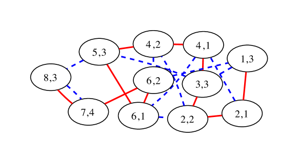
(c) Multiply-linked list

Figure 1: Row-reordering example with Multiple Lists

For our experiments, we applied Multiple Lists with $K=c$ as follows. First sort the table lexicographically after ordering the columns by non-decreasing cardinalities ($N_{1}\leq N_{2}\leq\dots\leq N_{c}$). Then rotate the columns cyclically so that the first column becomes the second one, the second one becomes the third one, and the last column becomes the first: $1,2,\dots,c\rightarrow c,1,2,\dots,c-1$. Sort the table lexicographically according to this new column order. Repeat this process until you have $c$ different orders, each one corresponding to the same table sorted lexicographically with a different column order.

Once we have sorted the table several times, we proceed as in Nearest Neighbor (see Algorithm 1):

Start with an initially empty list $\beta$.

Pick a row at random, remove it from all sorted lists and add it to list $\beta$.

In all sorted lists, visit all rows that are immediately adjacent (in sorted order) to the last row added. There are up to $2c$ such rows. Pick a nearest neighbor under the Hamming distance, remove it from all sorted lists and append it to $\beta$.

Repeat the last step until the sorted lists are empty. The solution is then given by list $\beta$, which now contains all rows.

Multiple Lists runs in time $O(Kcn\log n)$, or $O(c^{2}n\log n)$ when we use $c$ sorted lists. However, we can do better in the $K=c$ case with cyclically rotated column order. First, we sort with column order $1,2,\dots,c$ in $O(cn\log n)$ time. Then, we have $N_{1}$ lists—one list per value in the first column—sorted in the $c,1,2,\dots,c-1$-lexicographical order. Thus, sorting in the $c,1,2,\dots,c-1$-lexicographical order requires only $O(cn\log N_{1})$ time. Similarly, sorting in the $c-1,c,1,2,\dots,c-2$-lexicographical order requires $O(cn\log N_{2})$ time. And so on. Thus, the total sorting time is in

$$O(cn\log n+cn\log N_{1}+\dots+cn\log N_{c})=O(cn\log(nN_{1}N_{2}\dots N_{c-1})).$$

We expect that $nN_{1}N_{2}\dots N_{c-1}\ll n^{c}$ and thus

$$\log(nN_{1}N_{2}\dots N_{c-1})\ll c\log n$$

in practice. (This approach of reusing previous sorting orders when re-sorting is reminiscent of the Pipe Sort algorithm [Agarwal et al. (1996)].) The overall complexity of Multiple Lists is thus $O(c^{2}n+cn\log(nN_{1}N_{2}\dots N_{c-1}))$.

1:  input: Unsorted table $t$ with $n$ rows and $c$ columns.

2:  output: a sorted table

3:  Form $K$ different versions of $t$, sorted differently: $t^{(1)},t^{(2)},\dots,t^{(K)}$

4:  $\beta\leftarrow$ empty list

5:  pick an element in $t^{(1)}$ randomly, add it to $\beta$ and remove it from all $t^{(i)}$’s

6:  while $\mathrm{size}(\beta)<n$  do

7:     let $r$ be the latest element added to $\beta$

8:     Given $i\in\{1,2,\dots,K\}$, there are up to two neighbors in sorted order within list $t^{(i)}$; out of up to $2K$ such neighbors, pick a nearest neighbor $r^{\prime}$ to $r$ in Hamming distance.

9:     Add $r^{\prime}$ to $\beta$ and remove it from all $t^{(i)}$’s

10:  end while

11:  return $\beta$

Algorithm 1 The Multiple Lists heuristic

Although an increase in $K$ degrades the running time, we expect each new list stored to improve the solution’s quality. In fact, the heuristic Multiple Lists becomes equivalent to Nearest Neighbor when we maintain the table in all of the $c!$ lexicographical sorting orders. This shows the following result:

Lemma 3.5.

The Nearest Neighbor heuristic over $c$-column tables and under the Hamming distance is in $O(c\,c!\,n\log n)$.

When there are many columns ($c>4$), constructing and maintaining $c!$ lists might be prohibitive. Through informal tests, we found that maintaining $c$ different sort orders is a good compromise. For $c\leq 2$, Multiple Lists with $c$ sorted lists is already equivalent to Nearest Neighbor.

Unfortunately, our implementation of Multiple Lists is not suited to an external-memory implementation without partitioning.

3.3.2 Partitioning

Several authors partition—or cluster—the tuples before applying a TSP heuristic. [Cesari (1996), Reinelt (1994), Karp (1977), Johnson et al. (2004), Schaller (1999)] Using database terminology, they partition the table horizontally. We explore this approach. The content of the horizontal partitions depends on the original order of the rows: the first rows are in the first partition and so on. Hence, we are effectively considering a tour-improvement technique: starting from an existing row ordering, we partition it and try to reduce the number of runs within each partition. For example, we can partition a lexicographically sorted table and process each partition in main memory using expensive heuristics such as Nearest Neighbor or random-access-intensive heuristics such as Multiple Lists.

We can process each partition independently: the problem is embarrassingly parallel. Of course, this ignores runs created at the boundary between partitions.

Sometimes, we know the final row of the previous partition. In such cases, we might choose the initial row in the current partition to have a small Hamming distance with the last row in the previous partition. In any case, this boundary effect becomes small as the sizes of the partitions grow.

Another immediate practical benefit of the horizontal partitioning is that we have an anytime—or interruptible—algorithm [Dean and Boddy (1988)]. Indeed, we progressively improve the row ordering, but can also abort the process at any time without losing the gains achieved up to that point.

We could ensure that the number of runs is always reduced. Indeed, whenever the application of the heuristic on the partition makes matter worse, we can revert back to the original tuple order. Similarly, we can try several heuristics on each partition and pick the best. And probabilistic heuristics such as Nearest Neighbor can be repeated. Moreover, we can repartition the table: e.g., each new partition—except the first and the last—can take half its tuples from each of the two adjacent old partitions [Johnson and McGeoch (1997)].

For simplicity, we can use partitions having a fixed number of rows (except maybe for the last partition). As an alternative, we could first sort the data and then create partitions based on the value of one or several columns. Thus, for example, we could ensure that all rows within a partition have the same value in one or several columns.

4 Maximizing the number of long runs

It is convenient to model database compression by the number of runs (RunCount). However, this model is clearly incomplete. For example, there is some overhead corresponding to each run of values we need to code: short runs are difficult to compress.

4.1 Heuristics for long runs

We developed a number of row-reordering heuristics whose goal was to produce long runs. Two straightforward approaches did not give experimental results that justified their costs.

One is due to an idea of malik2007optimizing. Consider the Nearest Neighbor TSP heuristic. Because we use the Hamming distance, there are often several nearest neighbors for the last tuple added. Malik and Kender proposed a modification of Nearest Neighbor where they determine the best nearest neighbor based on comparisons with the previous tuples—and not only with the latest one. We considered many variations on this idea, and none of them proved consistently beneficial: e.g., when there are several nearest neighbors to the latest tuple, we tried reducing the set to a single tuple by removing the tuples that are not also nearest to the second last tuple, and then removing the tuples that are not also nearest to the third last tuple, and so on.

A novel heuristic, Iterated Matching, was also developed but found to be too expensive for the quality of results typically obtained. It is based on the observation that a weighted-matching algorithm can form pairs of rows that have many length-two runs. Pairs of rows can themselves be matched into collections of four rows with many length-four runs, etc. Unfortunately, known maximum-matching algorithms are expensive and the experimental results obtained with this heuristic were not promising. Details can be found elsewhere [Lemire et al. (2012)].

4.2 The Frequent-Component order

Intuitively, we would like to sort rows so that frequent values are more likely to appear consecutively. The Frequent-Component [Lemire et al. (2010)] order follows this intuition.

As a preliminary step, we compute the frequency $f(v)$ of each column value $v$ within each of the $c$ columns. Given a tuple, we map each component to the triple (frequency, column index, column value). Thus, from the $c$ components, we derive $c$ triples (see Figs. 2a and 2b): e.g., given the tuple $(v_{1},v_{2},v_{3})$, we get the triples $((f(v_{1}),1,v_{1}),(f(v_{2}),2,v_{2}),(f(v_{3}),3,v_{3}))$. We then lexicographically sort the triples, so that the triple corresponding to a most-frequent column value appears first—that is, we sort in reverse lexicographical order (see Fig. 2c): e.g., assuming that $f(v_{3})<f(v_{1})<f(v_{2})$, the triples appear in sorted order as $((f(v_{2}),2,v_{2}),(f(v_{1}),1,v_{1}),(f(v_{3}),3,v_{3}))$. The new tuples are then compared against each other lexicographically over the $3c$ values (see Fig. 2d). When sorting, we can precompute the ordered lists of triples for speed. As a last step, we reconstruct the solution from the list of triples (see Fig. 2e).

Consider a table where columns have uniform histograms: given $n$ rows and a column of cardinality $N_{i}$, each value appears $n/N_{i}$ times. In such a case, Frequent-Component becomes equivalent to the lexicographic order with the columns organized in non-decreasing cardinality.

1	3
2	1
2	2
3	3
4	1
4	2
5	3
6	1
6	2
7	4
8	3

(a) Initial table

(1,1,1)	(4,2,3)
(2,1,2)	(3,2,1)
(2,1,2)	(3,2,2)
(1,1,3)	(4,2,3)
(2,1,4)	(3,2,1)
(2,1,4)	(3,2,2)
(1,1,5)	(4,2,3)
(2,1,6)	(3,2,1)
(2,1,6)	(3,2,2)
(1,1,7)	(1,2,4)
(1,1,8)	(4,2,3)

(b) $(f(v_{i}),i,v_{i})$

(4,2,3)	(1,1,1)
(3,2,1)	(2,1,2)
(3,2,2)	(2,1,2)
(4,2,3)	(1,1,3)
(3,2,1)	(2,1,4)
(3,2,2)	(2,1,4)
(4,2,3)	(1,1,5)
(3,2,1)	(2,1,6)
(3,2,2)	(2,1,6)
(1,2,4)	(1,1,7)
(4,2,3)	(1,1,8)

(c) $(f(v_{i}),i,v_{i})$ (sorted)

(1,2,4)	(1,1,7)
(3,2,1)	(2,1,2)
(3,2,1)	(2,1,4)
(3,2,1)	(2,1,6)
(3,2,2)	(2,1,2)
(3,2,2)	(2,1,4)
(3,2,2)	(2,1,6)
(4,2,3)	(1,1,1)
(4,2,3)	(1,1,3)
(4,2,3)	(1,1,5)
(4,2,3)	(1,1,8)

(d) Sorted triples

7	4
2	1
4	1
6	1
2	2
4	2
6	2
1	3
3	3
5	3
8	3

(e) Solution

Figure 2: Row-reordering example with Frequent-Component

4.3 Vortex: a novel order

The Frequent-Component order has at least two inconveniences:

Given $c$ columns having $N$ distinct values apiece, a table where all possible rows are present has $N^{c}$ distinct rows. In this instance, Frequent-Component is equivalent to the lexicographic order. Thus, its RunCount is $N^{c}+N^{c-1}+\dots+1$. Yet a better solution would be to sort the rows in a Gray-code order, generating only $N^{c}+c-1$ runs. For mathematical elegance, we would rather have Gray-code orders even though the Gray-code property may not enhance compression in practice.

The Frequent-Component order requires comparisons between the frequencies of values that are in different columns. Hence, we must at least maintain one ordered list of values from all columns. We would prefer a simpler alternative with less overhead.

Thus, to improve over Frequent-Component, we want an order that considers the frequencies of column values and yet is a Gray-code order. Unlike Frequent-Component, we would prefer that it compare frequencies only between values from the same column.

1	1
1	2
1	3
1	4
2	1
2	2
2	3
2	4
3	1
3	2
3	3
3	4
4	1
4	2
4	3
4	4

(a) Lexicographic

1	1
1	2
1	3
1	4
2	4
2	3
2	2
2	1
3	1
3	2
3	3
3	4
4	4
4	3
4	2
4	1

(b) Reflected GC

1	4
1	3
1	2
1	1
4	1
3	1
2	1
2	4
2	3
2	2
4	2
3	2
3	4
3	3
4	3
4	4

(c) Vortex

1	1
1	2
2	2
2	1
2	3
2	4
1	4
1	3
3	3
3	4
4	4
4	3
4	1
4	2
3	2
3	1

(d) z-order with Gray codes

1	1
2	1
2	2
1	2
1	3
1	4
2	4
2	3
3	3
3	4
4	4
4	3
4	2
3	2
3	1
4	1

(e) Hilbert

Figure 3: Two-column tables sorted in various orders

Many orders, such as z-orders with Gray codes [Faloutsos (1986)] (see Fig. 3d) and Hilbert orders [Hamilton and Rau-Chaplin (2008), Kamel and Faloutsos (1994), Eavis and Cueva (2007)] (see Fig. 3e), use some form of bit interleaving: when comparing two tuples, we begin by comparing the most significant bits of their values before considering the less significant bits. Our novel Vortex order interleaves individual column values instead (see Fig. 3c). Informally, we describe the order as follows:

• Pick a most frequent value $x^{(1)}$ from the first column, select all tuples having the value $x^{(1)}$ as their first component, and put them first (see Fig. 5b with $x^{(1)}=1$);

• Consider the second column. Pick a most frequent value $y^{(1)}$. Among the tuples having $x^{(1)}$ as their first component, select all tuples having $y^{(1)}$ as their second component and put them last. Among the remaining tuples, select all tuples having $y^{(1)}$ as their second component, and put them first (see Fig. 5c with $y^{(1)}=1$);

• Repeat.

Our intuition is that, compared to bit interleaving, this form of interleaving is more likely to generate runs of identical values. The name Vortex comes from the fact that initially there are long runs, followed by shorter and shorter runs (see Figs. 3c and 4).

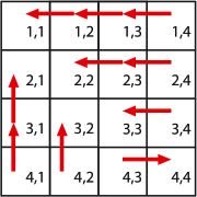
Figure 4: Graphical representation of some of the order relations between tuples in $\{1,2,3,4\}\times\{1,2,3,4\}$ under the Vortex order

2	1
1	1
1	2
1	1
3	1
1	3
3	2
3	3

(a) Shuffled

1	1
1	2
1	1
1	3
3	2
3	3
2	1
3	1

(b) Value 1, first column

1	2
1	3
1	1
1	1
2	1
3	1
3	2
3	3

(c) Value 1, second column

Figure 5: First two steps in sorting with Vortex

To describe the Vortex order formally (see Algorithm 2), we introduce the alternating lexicographic order (henceforth alternating). Given two tuples $a$ and $b$, let $j$ be the first component where the two tuples differ ($a_{j}\neq b_{j}$ but $a_{i}=b_{i}$ for $i<j$), then $a<_{\mbox{\tiny ALT}}b$ if and only if $(a_{j}<b_{j})\oplus(j\textrm{ is even})$ where $\oplus$ is the exclusive or. (We use the convention that components are labeled from 1 to $c$ so that the first component is odd.) Given a tuple $x=(x_{1},x_{2},\dots,x_{c})$, let $T(x)$ be $(x_{1},1),(x_{2},2),\ldots,(x_{c},c)$ and $T^{\prime}(x)$ be the list $T(x)$ sorted lexicographically. Then $x<_{\mbox{\tiny VORTEX}}y$ if and only if $T^{\prime}(x)<_{\mbox{\tiny ALT}}T^{\prime}(y)$. Vortex generates a total order on tuples because $T^{\prime}$ is bijective and alternating is a total order.

We illustrate Vortex sorting in Fig. 6. First, the initial table is normalized by frequency so that the most frequent value in each column is mapped to value 1 (see Figs. 6a, 6b, 6c). In Fig. 6d, we give the corresponding $T^{\prime}$ values: e.g., the row $1,4$ becomes $(1,2),(4,1)$. We then sort the $T^{\prime}$ values using the alternating order (see Fig. 6e) before finally inverting the $T^{\prime}$ values to recover the rows in Vortex order (see Fig. 6f). Of course, these are not the rows of the original table, but rather the rows of renormalized table. We could further reverse the normalization to recover the initial table in Vortex order.

1	3
2	1
2	2
3	3
4	1
4	2
5	3
6	1
6	2
7	4
8	3

(a) Initial table

column 1	column 2
$2\rightarrow 1$	$3\rightarrow 1$
$4\rightarrow 2$	$1\rightarrow 2$
$6\rightarrow 3$	$2\rightarrow 3$
$1\rightarrow 4$	$4\rightarrow 4$
$3\rightarrow 5$
$5\rightarrow 6$
$7\rightarrow 7$
$8\rightarrow 8$

(b) Renormalization

4	1
1	2
1	3
5	1
2	2
2	3
6	1
3	2
3	3
7	4
8	1

(c) Normalized table

$(1,2),(4,1)$
$(1,1),(2,2)$
$(1,1),(3,2)$
$(1,2),(5,1)$
$(2,1),(2,2)$
$(2,1),(3,2)$
$(1,2),(6,1)$
$(2,2),(3,1)$
$(3,1),(3,2)$
$(4,2),(7,1)$
$(1,2),(8,1)$

(d) $T^{\prime}$ values

$(1,1),(3,2)$
$(1,1),(2,2)$
$(1,2),(8,1)$
$(1,2),(6,1)$
$(1,2),(5,1)$
$(1,2),(4,1)$
$(2,1),(3,2)$
$(2,1),(2,2)$
$(2,2),(3,1)$
$(3,1),(3,2)$
$(4,2),(7,1)$

(e) alternating order

1	3
1	2
8	1
6	1
5	1
4	1
2	3
2	2
3	2
3	3
7	4

(f) Solution (normalized)

Figure 6: Row-reordering example with Vortex

Like the lexicographical order, the Vortex order is oblivious to the column cardinalities $N_{1},N_{2},\ldots,N_{c}$: we only use the content of the two tuples to determine which is smallest (see Algorithm 2).

1:  input: two tuples $x=(x_{1},x_{2},\ldots,x_{c})$ and $y=(y_{1},y_{2},\ldots,y_{c})$

2:  output: whether $x<_{\mbox{\tiny VORTEX}}y$

3:  $x^{\prime}\leftarrow(x_{1},1),(x_{2},2),\ldots,(x_{c},c)$

4:  sort the list $x^{\prime}$ lexicographically {E.g., $(13,1),(12,2)\rightarrow(12,2),(13,1)$.}

5:  $y^{\prime}\leftarrow(y_{1},1),(y_{2},2),\ldots,(y_{c},c)$

6:  sort the list $y^{\prime}$ lexicographically

7:  for $i=1,2,\ldots,c$ do

8:     if $x^{\prime}_{i}\neq y^{\prime}_{i}$  then

9:        return $(x^{\prime}_{i}<_{\mbox{\tiny LEXICO}}y^{\prime}_{i})\oplus(i\textrm{ is even})$

10:     end if

11:  end for

12:  return $\mathrm{false}$ {We have $x=y$.}

Algorithm 2 Comparison between two tuples of integers by the Vortex order. We recommend organizing the columns in non-decreasing order of cardinality and the column values in non-increasing order of frequency.

Compared with Frequent-Component, Vortex always chooses the first (most frequent) value from column 1, then the most frequent value from column 2, and so forth. Indeed, we can easily show the following proposition using the formal definition of the Vortex order:

Lemma 4.1.

Consider tuples with positive integer values. For any $1\leq k\leq c$, suppose $\tau$ is a tuple containing the value 1 in one of its first $k$ components, and $\tau^{\prime}$ is a tuple that does not contain the value 1 in any of its first $k$ components. Then $\tau<_{\mbox{\tiny VORTEX}}\tau^{\prime}$.

Frequent-Component instead chooses the most frequent value overall, then the second-most frequent value overall, and so forth, regardless of which column contains them. Both Frequent-Component and Vortex list all tuples containing the first value consecutively. However, whereas Vortex also lists the tuples containing the second value consecutively, Frequent-Component may fail to do so. Thus, we expect Vortex to produce fewer runs among the most frequent values, compared to Frequent-Component.

Whereas the Hilbert order is only a Gray code when $N$ is a power of two, we want to show that Vortex is always an $N$-ary Gray code. That is, sorting all of the tuples in $\{1,2,\dots,N\}\times\dots\times\{1,2,\dots,N\}=\{1,2,\dots,N\}^{c}$ creates a Gray code—the Hamming distance of successive tuples is one. We believe that of all possible orders, we might as well pick those with the Gray-code property, everything else being equal.

Let $\mathrm{\textsc{Vortex}}({N_{1},N_{2},\ldots,N_{c}})$ be the $\prod_{i=1}^{c}N_{i}$ tuples in $\{1,2,\dots,N_{1}\}\times\dots\times\{1,2,\dots,N_{c}\}$ sorted in the Vortex order. Let

$$\Lambda_{c,k}^{N}=\mathrm{\textsc{Vortex}}(\underbrace{N,N,\dots,N}_{c-k},\underbrace{N-1,N-1,\ldots,N-1}_{k}).$$

We begin by the following technical lemmata which allow us to prove that Vortex is a Gray code by induction.

Lemma 4.2.

If $\Lambda_{c-1,k-1}^{N}$ and $\Lambda_{c,k}^{N}$ are Gray codes, then so is $\Lambda_{c,k-1}^{N}$ for any integers $N>1$, $c\geq 2$, $k\in\{1,\dots,c\}$.

Proof 4.3.

Assume that $\Lambda_{c-1,k}^{N}$ and $\Lambda_{c,k}^{N}$ are Gray codes. The $\Lambda_{c,k-1}^{N}$ tuples begin with the tuple

$$(1,\underbrace{N,\ldots,N}_{c-k},\underbrace{N-1,N-1,\ldots,N-1}_{k-1})$$

and they continue up to the tuple

$$(1,1,\underbrace{N,\ldots,N}_{c-k-1},\underbrace{N-1,N-1,\ldots,N-1}_{k-1}).$$

Except for the first column which has a fixed value (one), these tuples are in reverse $\Lambda_{c-1,k-1}^{N}$ order, so they form a Gray code. The next tuple in $\Lambda_{c,k-1}^{N}$ is

$$(N,1,\underbrace{N,\ldots,N}_{c-k-1},\underbrace{N-1,N-1,\ldots,N-1}_{k-1})$$

and the following tuples are in an order equivalent to $\Lambda_{c,k}^{N}$, except that we must consider the first column as the last and decrement its values by one, while the second column is considered the first, the third column the second, and so on. The proof concludes.

Lemma 4.4.

For all $c\geq 1$ and all $k\in\{0,1,\ldots,c\}$, $\Lambda_{c,k}^{2}$ is a Gray code.

Proof 4.5.

We have that $\Lambda_{c,0}^{2}$ is a reflected Gray code with column values 1 and 2: e.g., for $c=3$, we have the order

$$\Lambda_{3,0}^{2} = \begin{matrix}1,2,2\\ 1,2,1\\ 1,1,1\\ 1,1,2\\ 2,1,2\\ 2,1,1\\ 2,2,1\\ 2,2,2\\ \end{matrix}.$$

Thus, we have that $\Lambda_{c,0}^{2}$ is always a Gray code. Any column with cardinality one can be trivially discarded. Hence, we have that $\Lambda_{c,k}^{2}$ is always a Gray code for all $k\in\{0,1,\ldots,c\}$, proving the lemma.

Lemma 4.6.

For any value of $N$ and for $k=0$ or $k=1$, $\Lambda_{1,k}^{N}$ is a Gray code.

Proof 4.7.

We have that $\Lambda_{1,0}^{N}$ is a Gray code for any value of $N$ because one-component tuples are always Gray codes. It immediately follows that $\Lambda_{1,1}^{N}$ is also a Gray code for any $N$ since, by definition, $\Lambda_{1,1}^{N}=\Lambda_{1,0}^{N-1}$.

Proposition 4.8.

The Vortex order is an $N$-ary Gray code.

Proof 4.9.

The proof uses a multiple induction argument, which we express as pseudocode. At the end of each pass through the loop on $N$, we have that $\Lambda_{c,k}^{N^{\prime}}$ is a Gray code for all $N^{\prime}\leq N$, all $c\in\{2,\dots,\mathcal{C}\}$ and all $k\in\{0,1,2,\ldots,c\}$. The induction begins from the cases where there are only two values per column ($N=2$, see Lemma 4.4) or only one column ($c=1$, Lemma 4.6). See Fig. 7 for an illustration.

1:  for $N=3,4,\ldots,\mathcal{N}$ do

2:     We have that $\Lambda_{c,k}^{N-1}$ is a Gray code for all $c\in\{2,3,\dots,\mathcal{C}\}$ and also for all $k\in\{0,1,2,\ldots,c\}$. {For $N>3$, this is true from the previous pass in the loop on $N$. For $N=3$, it follows from Lemma 4.4.}

3:     for $c=2,\dots,\mathcal{C}$ do

4:        By line 2, $\Lambda_{c,0}^{N-1}$ is a Gray code, and by definition $\Lambda_{c,c}^{N}=\Lambda_{c,0}^{N-1}$.

5:        for $k=c,c-1,\dots,1$ do

6:           (1) $\Lambda_{c,k}^{N}$ is a Gray code {when $k=c$ it follows by line 4 and otherwise by line 8 from the previous pass of the loop on $k$}

7:           (2) $\Lambda_{c-1,k-1}^{N}$ is a Gray code {when $c=2$, it follows by Lemma 4.6, and for $c>2$ it follows from the previous pass of the loop on $c$}

8:           (1) + (2) $\Rightarrow$ $\Lambda_{c,k-1}^{N}$ is a Gray code by Lemma 4.2.

9:        end for

10:        Hence, $\Lambda_{c,0}^{N}$ is a Gray code. (And also $\Lambda_{c,k}^{N}$ for all $k\in\{0,1,2,\ldots,c-1\}$.)

11:     end for

12:  end for

	$c=1$	$c=2$	$\cdots$	$\mathcal{C}$
$N=2$	Lemma 4.4
$N=3$	Lemma 4.6	$\rightarrow$	$\rightarrow$
$\vdots$		$\vdots$	$\vdots$
$\mathcal{N}$		$\rightarrow$	$\rightarrow$

Figure 7: Illustration of the basis for the induction argument in the proof of Proposition 4.8

The integers $\mathcal{N}$ and $\mathcal{C}$ can be arbitrarily large. Thus, the pseudocode shows that $\Lambda_{c,k}^{N}$ is always a Gray code which proves that Vortex is an $N$-ary Gray code for any number of columns and any value of $N$.

5 Experiments: TSP and synthetic data

We present two groups of experiments. In this section, we use synthetic data to compare many heuristics for minimizing RunCount. Because the minimization of RunCount reduces to the TSP over the Hamming distance, we effectively assess TSP heuristics. Two heuristics stand out, and then in § 6 these two heuristics are assessed in more realistic settings with actual database compression techniques and large tables. The Java source code necessary to reproduce our experiments is at http://code.google.com/p/rowreorderingjavalibrary/.

The aHDO scheme runs a complete pass through the table, trying to permute successive rows. If a pair of rows is permuted, we run through another pass over the entire table. We repeat until no improvement is possible. In contrast, the more expensive tour-improvement heuristics (BruteForcePeephole and 1-reinsertion) do a single pass through the table. The BruteForcePeephole is applied on successive blocks of 8 rows.

5.1 Reducing the number of runs on Zipfian tables

Zipfian distributions are commonly used [Eavis and Cueva (2007), Houkjær et al. (2006), Gray et al. (1994)] to model value distributions in databases: within a column, the frequency of the $i^{\mathrm{th}}$ value is proportional to $1/i$. If a table has $n$ rows, we allow each column to have $n$ possible distinct values, not all of which will usually appear. We generated tables with 8 192–1 048 576 rows, using four Zipfian-distributed columns that were generated independently. Applying Lemma 3.1 to these tables, the lexicographical order is $\omega$-optimal for $\omega\approx 3$.

Relative reduction in RunCount compared to lexicographical sort (set at 1.0), for Zipfian tables ($c=4$) relative RunCount reduction $n=$8 192 $n=$131 072 $n=1\,048\,576$ Lexicographic Sort 1.000 1.000 1.00 Multiple Lists 1.167 1.188 1.204 Vortex 1.154 1.186 1.203 Frequent-Component 1.151 1.186 1.203 Nearest Neighbor 1.223 1.242 Savings 1.225 1.243 Multiple Fragment 1.219 1.232 Farthest Insertion 1.187 Nearest Insertion 1.214 Random Insertion 1.201 Lexicographic Sort+1-reinsertion 1.171 Vortex+1-reinsertion 1.193 Frequent-Component+1-reinsertion 1.191

The RunCount results are presented in Table 5.1. We present relative RunCount reduction values: a value of 1.2 means that the heuristic is 20% better than lexicographic sort. For some less scalable heuristics, we only give results for small tables. Moreover, we omit results for aHDO [Malik and Kender (2007)] and BruteForcePeephole (with partitions of eight rows) because these tour-improvement heuristics failed to improve any tour by more than 1%. Because BruteForcePeephole fails, we conclude that all heuristics we consider are “locally almost optimal” because you cannot improve them appreciably by optimizing subsets of 8 consecutive rows.

Both Frequent-Component and Vortex are better than the lexicographic order. The Multiple Lists heuristic is even better but slower. Other heuristics such as Nearest Neighbor, Savings, Multiple Fragment and the insertion heuristics are even better, but with worse running time complexity. For all heuristics, the run-reduction efficiency grows with the number of rows.

5.2 Reducing the number of runs on uniformly distributed tables

We also ran experiments using uniformly distributed tables, generating $n$-row tables where each column has $n$ possible values. Any value within the table can take one of $n$ distinct values with probability $1/n$. For these tables, the lexicographical order is 3.6-optimal according to Lemma 3.1.

Table 5.2 summarizes the results. The most striking difference with Zipfian tables is that the efficiency of most heuristics drops drastically. Whereas Vortex and Frequent-Component are 20% superior to the lexicographical order on Zipfian data, they are barely better (2%) on uniformly distributed data. Moreover, we fail to see improved gains as the tables grow larger—unlike the Zipfian case. Intuitively, a uniform model implies that there are fewer opportunities to create long runs of identical values in several columns, when compared to a Zipfian model. This probably explains the poor performance of Vortex and Frequent-Component.

We were surprised by how well Multiple Lists performed on uniformly distributed data, even for small $n$. It fared better than most heuristics, including Nearest Neighbor, by beating lexicographic sort by 13%. Since Multiple Lists is a variant of the greedy Nearest Neighbor that considers a subset of the possible neighbors, we see that more choice does not necessarily give better results. Multiple Lists is a good choice for this problem.

Relative reduction in RunCount compared to lexicographical sort (set at 1.0), for uniformly distributed tables ($c=4$) relative RunCount reduction $n=$8 192 $n=$131 072 $n=1\,048\,576$ Lexicographic Sort 1.000 1.000 1.00 Multiple Lists 1.127 1.128 1.128 Vortex 1.020 1.020 1.021 Frequent-Component 1.022 1.023 1.023 Nearest Neighbor 1.122 1.123 Savings 1.122 1.123 Multiple Fragment 1.133 1.133 Farthest Insertion 1.075 Nearest Insertion 1.129 Random Insertion 1.103 Lexicographic Sort+1-reinsertion 1.092 Vortex+1-reinsertion 1.094 Frequent-Component+1-reinsertion 1.080

5.3 Discussion

For these in-memory synthetic data sets, we find that the good heuristics to minimize RunCount—that is, to solve the TSP under the Hamming distance—are Vortex and Multiple Lists. They are both reasonably scalable in the number of rows ($O(n\log n)$) and they perform well as TSP heuristics.

Frequent-Component would be another worthy alternative, but it is harder to implement as efficiently as Vortex. Similarly, we found that Savings and Multiple Fragment could be superior TSP heuristics for Zipfian and uniformly distributed tables, but they scale poorly with respect to the number of rows: they have a quadratic running time ($O(n^{2})$). For small tables ($n=131\,072$), they were three and four orders of magnitude slower than Multiple Lists in our tests.

6 Experiments with realistic tables

Minimizing RunCount on synthetic data might have theoretical appeal and be somewhat applicable to many applications. However, we also want to determine whether row-reordering heuristics can specifically improve table compression, and therefore database performance, on realistic examples. This requires that we move from general models such as RunCount to size measurements based on specific database-compression techniques. It also requires large real data sets.

6.1 Realistic column storage

We use conventional dictionary coding [Lemke et al. (2010), Binnig et al. (2009), Poess and Potapov (2003)] prior to row-reordering and compression. That is, we map column values bijectively to 32-bit integers in $[0,N)$ where $N$ is the number of distinct column values. We map the most frequent values to the smallest integers [Lemire and Kaser (2011)].

We compress tables using five database compression schemes: Sparse, Indirect and Prefix coding as well as a fast variation on Lempel-Ziv and RLE. We compare the compression ratio of each technique under row reordering. For simplicity, we select only one compression scheme at a time: all columns are compressed using the same technique.

6.1.1 Block-wise compression

The SAP NetWeaver platform [Lemke et al. (2010)] uses three compression techniques: Indirect, Sparse and Prefix coding. We implemented them and set the block size to $p=128$ values.

Indirect coding is a block-aware dictionary technique. For each column and each block, we build a list of the $N^{\prime}$ values encountered. Typically, $N^{\prime}\ll N$, where $N$ is the total number of distinct values in the column. Column values are then mapped to integers in $[0,N^{\prime})$ and packed using $\lceil\log N\rceil$ bits each [Ng and Ravishankar (1997), Binnig et al. (2009)]. Of course, we must also store the actual values of the $N^{\prime}$ codes used for each block and column. Thus, whereas dictionary coding requires $p\lceil\log N\rceil$ bits to store a column, Indirect coding requires $N^{\prime}\lceil\log N\rceil+p\lceil\log N^{\prime}\rceil$ bits—plus the small overhead of storing the value of $N^{\prime}$. In the worst case, the storage cost of indirect coding is twice as large as the storage cost of conventional dictionary coding. However, whenever $N^{\prime}$ is small enough, indirect coding is preferable. Indirect coding is related to the block-wise value coding used by Oracle [Poess and Potapov (2003)].

Sparse coding stores the most frequent value using an $p$-bit bitmap to indicate where this most frequent value appears. Other values are stored using $\lceil\log N\rceil$ bits. If the most frequent value appears $\zeta$ times, then the total storage cost is $(p-\zeta+1)\lceil\log N\rceil+p$ bits.

Prefix coding begins by counting how many times the first value repeats at the beginning of the block; this counter is stored first along with the value being repeated. Then all other values are packed. In the worst case, the first value is not repeated, and Prefix coding wastes $\lceil\log p\rceil$ bits compared to conventional dictionary coding. Because it counts the length of a run, Prefix coding can be considered a form of RLE (§ 6.1.3).

6.1.2 Lempel-Ziv-Oberhumer

Lempel-Ziv compression [Ziv and Lempel (1978)] compresses data by replacing sequences of characters by references to previously encountered sequences. The Lempel-Ziv-Oberhumer (LZO) library [Oberhumer (2011)] implements fast versions of the conventional Lempel-Ziv compression technique. 1142548 evaluated several alternatives including Huffman and Arithmetic encoding, but found that compared with LZO, they were all too expensive for databases.

If a long data array is made of repeated characters—e.g., aaaaa—or repeated short sequences—e.g., ababab—we expect most Lempel-Ziv compression techniques to generate a compressed output that grows logarithmically with the size of the input. It appears to be the case with the LZO library: its LZO1X CODEC uses 16 bytes to code 64 identical 32-bit integers, 17 bytes to code 128 identical integers, and 19 bytes for 256 integers. For our tests, we used LZO version 2.05.

6.1.3 Run-Length Encoding

We implemented RLE by storing each run as a triple [Stonebraker et al. (2005)]: value, starting point and length of the run. Values are packed using $\lceil\log N\rceil$ bits whereas both the starting point and the length of the run are stored using $\lceil\log n\rceil$ bits, where $n$ is the number of rows.

6.2 Data sets

Characteristics of data sets used with bounds on the optimality of lexicographical order ($\omega$), and a measure of statistical deviation ($p_{0}$). rows distinct rows cols $\sum_{i}N_{i}$ $\omega$ $p_{0}$ Census1881 4 277 807 4 262 238 7 343 422 2.9 0.17 Census-Income 199 523 196 294 42 103 419 12 0.65 Wikileaks 1 178 559 1 147 059 4 10 513 1.3 0.04 SSB (DBGEN) 240 012 290 240 012 290 15 8 874 195 8.0 0.10 Weather 124 164 607 124 164 371 19 52 369 4.5 0.36 USCensus2000 37 019 068 22 493 432 10 2 774 239 3.4 0.54

We selected realistic data sets (see Table 6.2): Census1881 [Lemire and Kaser (2011), Programme de recherche en démographie historique (2009)], Census-Income [Frank and Asuncion (2010)], a Wikileaks-related data set, the fact table from the Star Schema Benchmark (SSB) [O’Neil et al. (2009)] and Weather [Hahn et al. (2004)]. Census1881 comes from the Canadian census of 1881: it is over 305 MB and over 4 million records. Census-Income is the smallest data set with 100 MB and 199 523 records. However, it has 42 columns and one column has a very high relative cardinality (99 800 distinct values). The Wikileaks table was created from a public repository published by Google and it contains the non-classified metadata related to leaked diplomatic cables. We extracted 4 columns: year, time, place and descriptive code. It has 1 178 559 records. We generated the SSB fact table using a version of the DBGEN software modified by O’Neil. We used a scale factor of 40 to generate it: that is, we used command dbgen -s 40 -T l. It is 20 GB and includes 240 million rows. The largest non-synthetic data set (Weather) is 9 GB. It consists of 124 million surface synoptic weather reports from land stations for the 10-year period from December 1981 through November 1991. We also extracted a table from the US Census of 2000 [US Census Bureau (2002)] (henceforth USCensus2000). We used attributes 5 to 15 from summary file 3. The resulting table has 37 million rows.

The column cardinalities for Census1881 range from 138 to 152 882 and from 2 to 99 800 for Census-Income. Our Wikileaks table has column cardinalities 273, 1 440, 3 935 and 4 865. The SSB table has column cardinalities ranging from 1 to 6 084 386. (The fact table has a column with a single value in it: zero.) For Weather, the column cardinalities range from 2 to 28 767. Attribute cardinalities for USCensus2000 vary between 130 001 to 534 896.

For each data set, we give the suboptimality factor $\omega$ from Lemma 3.1 in Table 6.2. Wikileaks has the lowest factor ($\omega=1.3$) followed by Census1881 ($\omega=2.9$) whereas Census-Income has the largest one ($\omega=12.4$). Correspondingly, Wikileaks and Census1881 have the fewest columns (4 and 7), and Census-Income has the most (42).

We also provide a simple measure of the statistical dispersion of the frequency of the values. For column $i$, we find a most frequent value $v_{i}$, and we determine what fraction of this column’s values are $v_{i}$. Averaging the fractions, we have our measure $p_{0}=\sum_{i=1}^{c}f(v_{i})/nc$, where our table has $n$ rows and $c$ columns and $f(v_{i})$ is the number of times $v_{i}$ occurs in its column. As an example, consider the table in Fig. 1a. In the first column, the value ‘6’ is a most frequent value and it appears twice in 11 tuples. In the second column, the value ‘3’ is most frequent, and it appears 4 times. In this example, we have $p_{0}=\frac{2+4}{2\times 11}\approx 0.27$. In general, we have that $p_{0}$ ranges between 0 and 1. For uniformly distributed tables having high cardinality columns, the fraction $p_{0}$ is near zero. When there is high statistical dispersion of the frequencies, we expect that the most frequent values have high frequencies and so $p_{0}$ could be close to 1. One benefit of this measure is that it can be computed efficiently. By this measure, we have the highest statistical dispersion in Census-Income, Weather and USCensus2000.

6.3 Implementation

Because we must be able to process large files in a reasonable time, we selected Vortex as one promising row-reordering heuristic. We implemented Vortex in memory-conscious manner: intermediate tuples required for a comparison between rows are repeatedly built on-the-fly.

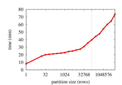
(a) Running time

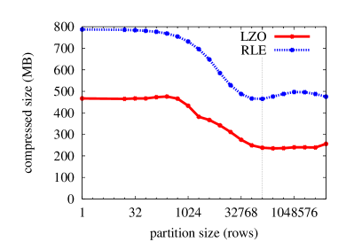
(b) Compressed data size

Figure 8: The Multiple Lists heuristic applied on each partition of a lexicographically sorted Weather table for various partition sizes. When partitions have size 1, we recover the lexicographical order. We refer to the case where the partition size is set to 131 072 rows as $\textsc{Multiple Lists}^{\star}$ (indicated by a dashed vertical line in the plots).

Prior to sorting lexicographically, we reorder columns in order of non-decreasing cardinality [Lemire and Kaser (2011)]: in all cases this was preferable to ordering the columns in decreasing cardinality. For Vortex, in all cases, there was no significant difference ($<1\%$) between ordering the columns in increasing or decreasing order of cardinality. Effectively, Vortex does not favor a particular column order. (A related property can be formally proved [Lemire et al. (2012)].)

We used Multiple Lists on partitions of a lexicographically sorted table (see § 3.3). Fig. 8 shows the effect of the partition size on both the running time and the data compression. Though larger partitions may improve compression, they also require more time. As a default, we chose partitions of 131 072 rows. Henceforth, we refer to this heuristic as $\textsc{Multiple Lists}^{\star}$.

We compiled our C++ software under GNU GCC 4.5.2 using the -O3 flag. The C++ source code is at http://code.google.com/p/rowreorderingcpplibrary/. We ran our experiments on an Intel Core i7 2600 processor with 16 GB of RAM using Linux. All data was stored on disk, before and after the compression. We used a 1 TB SATA hard drive with an estimated sustained reading speed of 115 MB/s. We used an external-memory sort that we implemented in the conventional manner [Knuth (1997)]: we load partitions of rows, which we sort in RAM and write back in the file; we then merge these sorted partitions using a priority queue. Our code is sequential.

Our algorithms are scalable. Indeed, both Vortex and lexicographical sorting rely on the standard external-memory sorting algorithm. The only difference between Vortex and lexicographical sort is that the function used to compare tuples is different. This difference does not affect scalability with respect to the number of tuples even though it makes Vortex slower. As for $\textsc{Multiple Lists}^{\star}$, it relies on external-memory sorting and the repeated application of Multiple Lists on fixed-sized blocks—both of which are scalable.

6.4 Experimental results on realistic data sets

We present the results in Table 6.4, giving the compression ratio on top of the lexicographical order: e.g., a value of two indicates that the compression ratio is twice as large as what we get with the lexicographical order.

Compression ratio compared to lexicographical sort

	Vortex	$\textsc{Multiple Lists}^{\star}$
Sparse	1.27	1.00
Indirect	1.07	1.02
Prefix	1.45	0.99
LZO	0.99	1.07
RLE	1.02	1.13
RunCount	0.99	1.13

(a) Census 1881

	Vortex	$\textsc{Multiple Lists}^{\star}$
	1.00	0.99
	1.03	0.96
	1.15	0.95
	0.97	1.04
	0.97	1.24
	0.96	1.25

(b) Census-Income

	Vortex	$\textsc{Multiple Lists}^{\star}$
Sparse	1.15	0.94
Indirect	0.63	0.96
Prefix	1.21	0.91
LZO	0.63	0.90
RLE	0.71	1.14
RunCount	0.70	1.14

(c) Wikileaks

	Vortex	$\textsc{Multiple Lists}^{\star}$
	1.00	0.99
	1.00	0.99
	1.00	0.97
	1.00	1.00
	1.00	1.00
	1.00	1.00

(d) SSB (DBGEN)

	Vortex	$\textsc{Multiple Lists}^{\star}$
Sparse	0.80	1.06
Indirect	0.78	1.55
Prefix	0.74	0.94
LZO	0.91	1.96
RLE	0.67	1.69
RunCount	0.66	1.67

(e) Weather

	Vortex	$\textsc{Multiple Lists}^{\star}$
	1.09	1.00
	1.72	1.06
	1.81	1.08
	0.26	0.94
	3.08	1.15
	3.04	1.15

(f) USCensus2000

Neither Vortex nor $\textsc{Multiple Lists}^{\star}$ was able to improve the compression ratio on the SSB data set. In fact, there was no change (within 1%) when replacing the lexicographical order with Vortex. And $\textsc{Multiple Lists}^{\star}$ made things slightly worse (by 3%) for Prefix coding, but left other compression ratios unaffected (within 1%). To interpret this result, consider that, while widely used, the DBGEN tool still generates synthetic data. For example, out of 17 columns, seven have almost perfectly uniform histograms. Yet “real world data is not uniformly distributed” [Poess and Potapov (2003)].

For Census1881, the most remarkable result is that Vortex was able to improve the compression under Sparse or Prefix coding by 27% and 45%. For Census-Income, $\textsc{Multiple Lists}^{\star}$ was able to improve RLE compression by 25%. For Wikileaks, we found it interesting that $\textsc{Multiple Lists}^{\star}$ reduced RunCount (and the RLE output) by 14% whereas the lexicographical order is already 1.26-optimal, which means that $\textsc{Multiple Lists}^{\star}$ is 1.1-optimal in this case. On Weather, the performance of Vortex was disappointing: it worsened the compression in all cases. However, $\textsc{Multiple Lists}^{\star}$ had excellent results: it doubled the Lempel-Ziv (LZO) compression, and it improved RLE compression by 70%. Yet on the USCensus2000 data set, Vortex was preferable to $\textsc{Multiple Lists}^{\star}$ for all compression schemes except LZO. We know that the lexicographical order is 3.4-optimal at reducing RunCount, yet Vortex is able to reduce RunCount by a factor of 3 compared to the lexicographical order. It follows that Vortex is 1.1-optimal in this case.

Overall, both Vortex and $\textsc{Multiple Lists}^{\star}$ can significantly improve over the lexicographic order when a database-compression technique is used on real data. For every database-compression technique, significant improvement could be obtained by at least one of the reordering heuristics on the real data sets. However, significant degradation could also be observed, and lexicographic order was best in four realistic cases (Sparse coding on Census-Income, Indirect coding on Wikileaks, Prefix coding on Weather and LZO on USCensus2000). In § 6.5, we propose to determine, based on characteristics of the data, whether significant gains are possible on top of the lexicographical order.

6.4.1 Our row-reordering heuristics are scalable

We present wall-clock timings in Table 6.4.1 to confirm our claims of scalability. For this test, we included a variation of the SSB where we used a scale factor of 100 instead of 40 when generating the data. That is, it is 2.5 times larger (henceforth SSB $\times 2.5$). As expected, the lexicographical order is fastest, whereas $\textsc{Multiple Lists}^{\star}$ is slower than either Vortex or the lexicographical order. On the largest data set (SSB), Vortex and $\textsc{Multiple Lists}^{\star}$ were 3 and 4 times slower than lexicographical sorting. One of the benefits of an approach based on partitions, such as $\textsc{Multiple Lists}^{\star}$, is that one might stop early if benefits are not apparent after a few partitions. When comparing SSB and SSB $\times 2.5$, we see that the running time grew by a factor of 4 for the lexicographical order, a factor of 2 for Vortex and a factor of 3 for $\textsc{Multiple Lists}^{\star}$. For SSB $\times 2.5$, the running time of $\textsc{Multiple Lists}^{\star}$ included 50 min for sorting the table lexicographically, and the application of Multiple Lists on blocks of rows only took 104 min. Because $\textsc{Multiple Lists}^{\star}$ uses blocks with a fixed size, its running time will be eventually dominated by the time required to sort the table lexicographically as we increase the number of tuples.

Time necessary to reorder the rows Lexico. Vortex $\textsc{Multiple Lists}^{\star}$ Census1881 $2.7$ s $14$ s $19$ s Census-Income $0.19$ s $4.7$ s $11$ s Wikileaks $0.3$ s $2.0$ s $2.5$ s SSB 12 min 35 min 52 min SSB $\times 2.5$ 49 min 105 min 154 min Weather 6 min 26 min 43 min USCensus2000 33 s 3 min 12 min

6.4.2 Better compression improves speed

Everything else being equal, if less data needs to be loaded from RAM and disk to the CPU, speed is improved. It remains to assess whether improved compression can translate into better speed in practice. Thus, we evaluated how fast we could uncompress all of the columns back into the original 32-bit dictionary values. Our test was to retrieve the data from disk (with buffering) and store it back on disk. We report the ratio of the decompression time with lexicographical sorting over the decompression time with alternative row reordering methods. Because the time required to write the decompressed values would have been unaffected by the compression, we would not expect speed gains exceeding 50% with better compression in this kind of test.

• First, we look at our good compression results on the Weather data set with $\textsc{Multiple Lists}^{\star}$ for the LZO and RLE (resp. 1.96 and 1.69 compression gain). The decompression speed was improved respectively by a factor of 1.19 and 1.14.

• Second, we consider the USCensus2000 table, where Vortex improved both Prefix coding and RLE compression (resp. 1.81 and 3.04 compression gain). We saw gains to the decompression speed of 1.04 and 1.12.

These speed gains were on top of the gains already achieved by lexicographical sorting. For example, Prefix coding was only improved by 4% compared to the lexicographical order on the USCensus2000 table, but if we compute ratios with respect to a shuffled table, they went from 1.25 for lexicographical sorting to 1.30 with Vortex. Hence, the total performance gain due to row reordering is 30%.

6.5 Guidance on selecting the row-reordering heuristic

It is difficult to determine which row-reordering heuristic is best given a table and a compression scheme. Our processing techniques are already fast, and useful guidance would need to be obtained faster—probably limiting us to decisions using summaries such as those maintained by the DBMS. And such concise summaries might be insufficient:

Suppose that we are given a set of columns and complete knowledge of their histograms. That is, we have the list of attribute values and their frequencies. Unfortunately, even given all this data, we could not predict the efficiency of the row reordering techniques reliably. Indeed, consider the USCensus2000 data set. According to Table 6.4, Vortex improves RLE compression by a factor of 3 over the lexicographical order. Consider what happened when we took the same table (USCensus2000) and randomly shuffled columns, independently. The column histograms were not changed—only the relationships between columns were affected. Yet, not only did Vortex fail to improve RLE compression over this newly generated table, it made it much worse (from a ratio of 3.04 to 0.74). The performance of $\textsc{Multiple Lists}^{\star}$ was also adversely affected: while it slightly improves the compression by Prefix coding (1.08) over the original USCensus2000 table, it made compression worse (0.93) over the reshuffled USCensus2000 table.

Perhaps one might hope to predict the efficiency of row-reordering techniques by using small samples, without ever sorting the entire table. There are reasons again to be pessimistic. We took a random sample of 65 536 tuples from the USCensus2000 table. Over such a sample, Vortex improved LZO compression by 2.5% compared to the lexicographical order, whereas over the whole data set Vortex makes LZO much worse than the lexicographical order (1.025 versus 0.26). Similarly, whereas Vortex improves RLE by a factor of 3 when applied over the whole table, the gain was far more modest over our sample (1.06 versus 3.04).

However, we can offer some guidance. For compression schemes that are closely related to RunCount, such as RLE, the optimality of a lexicographic sort should be computed using Lemma 3.1. If $\omega\approx 1$, we can safely conclude that the lexicographical order is sufficient.

Moreover, our results on synthetic data sets (§ 5) suggest that some statistical dispersion in the frequencies of the values is necessary. Indeed, we could not improve the RunCount of tables having uniformly distributed columns even when $\omega$ were relatively large. On our real data sets, we got the best compression gains compared to the lexicographical order with the Weather and USCensus2000 tables. They both have high $p_{0}$ values (0.36 and 0.54).

Hence, we propose to only try better row-reordering heuristics when $\omega$ and $p_{0}$ are large (e.g., $\omega>3$ and $p_{0}>0.3$). Both measures can be computed efficiently.

Furthermore, when applying a scheme such as Multiple Lists on partitions of the sorted table, it would be reasonable to stop the heuristic after a few partitions if there is no benefit. For example, consider the Weather data and $\textsc{Multiple Lists}^{\star}$. After 20 blocks of 131 072 tuples, we have a promising gain of 1.6 for LZO and RLE, but a disappointing ratio of 0.96 for Prefix coding. That is, we have valid estimates (within 10%) of the actual gain over the whole data set after processing only 2% of the table.

7 Conclusion

For the TSP under the Hamming distance, lexicographical sort is an effective and natural heuristic. It appears to be easier to surpass the lexicographical sort when the column histograms have high statistical dispersion (e.g. Zipfian distributions).

Our original question was whether engineers willing to spend extra time reordering rows could improve the compressibility of their tables, at least by a modest amount. Our answer is positive.

• Over real data, $\textsc{Multiple Lists}^{\star}$ always improved RLE compression when compared to the lexicographical order (10% to 70% better).

• Vortex almost always improved Prefix coding compression, sometimes by a large percentage (80%) compared to the lexicographical order.

• On one data set, Vortex improved RLE compression by a factor of 3 compared to lexicographical order.

As far as heuristics are concerned, we have certainly not exhausted the possibilities. Several tour-improvement heuristics used to solve the TSP [Johnson and McGeoch (1997)] could be adapted for row reordering. Maybe more importantly, we could adapt the TSP heuristics using a different distance measure than the Hamming distance. For example, consider difference coding [Moffat and Stuiver (2000), Bhattacharjee et al. (2009), Anh and Moffat (2010)] where the successive differences between attribute values are coded. In this case, we could use an inter-row distance that measures the number of bits required to code the differences. Just as importantly, the implementations of our row-reordering heuristics are sequential: parallel versions could be faster, especially on multicore processors.

M YM Y

References

- Abadi et al. (2006) Abadi, D., Madden, S., and Ferreira, M. 2006. Integrating compression and execution in column-oriented database systems. In Proceedings of the 2006 ACM SIGMOD International Conference on Management of Data. ACM, New York, NY, USA, 671–682.
- Abadi et al. (2008) Abadi, D. J., Madden, S. R., and Hachem, N. 2008. Column-stores vs. row-stores: how different are they really? In Proceedings of the 2008 ACM SIGMOD International Conference on Management of Data. ACM, New York, NY, USA, 967–980.
- Agarwal et al. (1996) Agarwal, S., Agrawal, R., Deshpande, P., Gupta, A., Naughton, J. F., Ramakrishnan, R., and Sarawagi, S. 1996. On the computation of multidimensional aggregates. In VLDB’96, Proceedings of the 22nd International Conference on Very Large Data Bases. Morgan Kaufmann, San Francisco, CA, USA, 506–521.
- Anantha et al. (2007) Anantha, M., Bose, B., and AlBdaiwi, B. 2007. Mixed-radix Gray codes in Lee metric. IEEE Trans. Comput. 56, 10, 1297–1307.
- Anh and Moffat (2010) Anh, V. N. and Moffat, A. 2010. Index compression using 64-bit words. Softw. Pract. Exper. 40, 2, 131–147.
- Antoshenkov (1995) Antoshenkov, G. 1995. Byte-aligned bitmap compression. In Data Compression Conference (DCC’95). IEEE Computer Society, Washington, DC, USA, 476.
- Aouiche and Lemire (2007) Aouiche, K. and Lemire, D. 2007. A comparison of five probabilistic view-size estimation techniques in OLAP. In Proceedings of the ACM 10th International Workshop on Data Warehousing and OLAP (DOLAP ’07). ACM, New York, NY, USA, 17–24.
- Applegate et al. (2003) Applegate, D., Cook, W., and Rohe, A. 2003. Chained Lin-Kernighan for large traveling salesman problems. INFORMS J. Comput. 15, 1, 82–92.
- Bellmore and Nemhauser (1968) Bellmore, M. and Nemhauser, G. L. 1968. The traveling salesman problem: a survey. Oper. Res. 16, 3, 538–558.
- Bentley (1992) Bentley, J. 1992. Fast algorithms for geometric traveling salesman problems. INFORMS J. Comput. 4, 4, 387–411.
- Berman and Karpinski (2006) Berman, P. and Karpinski, M. 2006. 8/7-approximation algorithm for (1,2)-TSP. In Proceedings of the 17th annual ACM-SIAM symposium on Discrete algorithms. ACM, New York, NY, USA, 641–648.
- Bhattacharjee et al. (2009) Bhattacharjee, B., Lim, L., Malkemus, T., Mihaila, G., Ross, K., Lau, S., McArthur, C., Toth, Z., and Sherkat, R. 2009. Efficient index compression in DB2 LUW. Proc. VLDB Endow. 2, 2, 1462–1473.
- Binnig et al. (2009) Binnig, C., Hildenbrand, S., and Färber, F. 2009. Dictionary-based order-preserving string compression for main memory column stores. In Proceedings of the 2009 ACM SIGMOD International Conference on Management of Data. ACM, New York, NY, USA, 283–296.
- Bruno (2009) Bruno, N. 2009. Teaching an old elephant new tricks. In Proceedings, CIDR 2009 : Fourth Biennial Conference on Innovative Data Systems. Asilomar, USA. electronic proceedings at https://database.cs.wisc.edu/cidr/cidr2009/cidr2009.zip, last checked 2012-07-04.
- Cai and Paige (1995) Cai, J. and Paige, R. 1995. Using multiset discrimination to solve language processing problems without hashing. Theor. Comput. Sci. 145, 1-2, 189–228.
- Cesari (1996) Cesari, G. 1996. Divide and conquer strategies for parallel TSP heuristics. Comput. Oper. Res. 23, 7, 681–694.
- Chakrabarti et al. (1999) Chakrabarti, A., Chazelle, B., Gum, B., and Lvov, A. 1999. A lower bound on the complexity of approximate nearest-neighbor searching on the Hamming cube. In Proceedings of the 31st annual ACM symposium on Theory of computing. ACM, New York, NY, USA, 305–311.
- Cho and Hong (2000) Cho, D.-S. and Hong, B.-H. 2000. Optimal page ordering for region queries in static spatial databases. In 11th International Conference on Database and Expert System Applications (DEXA’00), LNCS 1873. Springer, Berlin, Heidelberg, 366–375.
- Christofides (1976) Christofides, N. 1976. Worst-case analysis of a new heuristic for the travelling salesman problem. Tech. Rep. 388, Graduate School of Industrial Administration, Carnegie Mellon University.
- Clarke and Wright (1964) Clarke, G. and Wright, J. W. 1964. Scheduling of vehicles from a central depot to a number of delivery points. Oper. Res. 12, 4, 568–581.
- Croes (1958) Croes, G. A. 1958. A method for solving traveling-salesman problems. Oper. Res. 6, 6, 791–812.
- Dean and Boddy (1988) Dean, T. and Boddy, M. 1988. An analysis of time-dependent planning. In Proceedings of the 7th national conference on artificial intelligence. AAAI, Palo Alto, California, USA, 49–54.
- Ding et al. (2010) Ding, S., Attenberg, J., and Suel, T. 2010. Scalable techniques for document identifier assignment in inverted indexes. In Proceedings of the 19th International Conference on World Wide Web (WWW ’10). ACM, New York, NY, USA, 311–320.
- Eavis and Cueva (2007) Eavis, T. and Cueva, D. 2007. A Hilbert space compression architecture for data warehouse environments. In Data Warehousing and Knowledge Discovery (DaWaK’07) (LNCS 4654). Springer, Berlin, Heidelberg, 1–12.
- Ernvall et al. (1985) Ernvall, J., Katajainen, J., and Penttonen, M. 1985. NP-completeness of the Hamming salesman problem. Bit 25, 1, 289–292.
- Faloutsos (1986) Faloutsos, C. 1986. Multiattribute hashing using Gray codes. SIGMOD Rec. 15, 2, 227–238.
- Frank and Asuncion (2010) Frank, A. and Asuncion, A. 2010. UCI machine learning repository. http://archive.ics.uci.edu/ml (checked 2012-07-04).
- Fusco et al. (2010) Fusco, F., Stoecklin, M. P., and Vlachos, M. 2010. NET-FLi: On-the-fly compression, archiving and indexing of streaming network traffic. Proc. VLDB Endow. 3, 1382–1393.
- Fusco et al. (2012) Fusco, F., Vlachos, M., and Stoecklin, M. 2012. Real-time creation of bitmap indexes on streaming network data. VLDB J. 21, 3, 287–307.
- Gabow and Tarjan (1991) Gabow, H. N. and Tarjan, R. E. 1991. Faster scaling algorithms for general graph matching problems. J. ACM 38, 4, 815–853.
- Gharan et al. (2011) Gharan, S. O., Saberi, A., and Singh, M. 2011. A randomized rounding approach to the traveling salesman problem. In Proceedings of the 2011 IEEE 52nd Annual Symposium on Foundations of Computer Science. IEEE Computer Society, Washington, DC, USA, 550–559.
- Gionis et al. (1999) Gionis, A., Indyk, P., and Motwani, R. 1999. Similarity search in high dimensions via hashing. In VLDB’99, Proceedings of the 25th International Conference on Very Large Data Bases. Morgan Kaufmann, San Francisco, CA, USA, 518–529.
- Golomb (1966) Golomb, S. W. 1966. Run-length encodings. IEEE Trans. Inf. Theory 12, 3, 399–401.
- Gray et al. (1994) Gray, J., Sundaresan, P., Englert, S., Baclawski, K., and Weinberger, P. J. 1994. Quickly generating billion-record synthetic databases. SIGMOD Rec. 23, 2, 243–252.
- Grigoriadis and Kalantari (1988) Grigoriadis, M. D. and Kalantari, B. 1988. A new class of heuristic algorithms for weighted perfect matching. J. ACM 35, 4, 769–776.
- Hahn et al. (2004) Hahn, C., Warren, S., and London, J. 2004. Edited synoptic cloud reports from ships and land stations over the globe, 1982–1991. http://cdiac.ornl.gov/ftp/ndp026b/ (checked 2012-07-04).
- Hamilton and Rau-Chaplin (2008) Hamilton, C. H. and Rau-Chaplin, A. 2008. Compact Hilbert indices: Space-filling curves for domains with unequal side lengths. Inf. Process. Lett. 105, 5, 155–163.
- Helsgaun (2000) Helsgaun, K. 2000. An effective implementation of the Lin–Kernighan traveling salesman heuristic. Eur. J. Oper. Res. 126, 1, 106–130.
- Holloway and DeWitt (2008) Holloway, A. L. and DeWitt, D. J. 2008. Read-optimized databases, in depth. Proc. VLDB Endow. 1, 1, 502–513.
- Houkjær et al. (2006) Houkjær, K., Torp, K., and Wind, R. 2006. Simple and realistic data generation. In VLDB’06, Proceedings of the 32nd International Conference on Very Large Data Bases. ACM, New York, NY, USA, 1243–1246.
- Indyk and Motwani (1998) Indyk, P. and Motwani, R. 1998. Approximate nearest neighbors: towards removing the curse of dimensionality. In Proceedings of the 30th annual ACM symposium on Theory of computing. ACM, New York, NY, USA, 604–613.
- Indyk et al. (1997) Indyk, P., Motwani, R., Raghavan, P., and Vempala, S. 1997. Locality-preserving hashing in multidimensional spaces. In Proceedings of the 29th annual ACM symposium on Theory of computing. ACM, New York, NY, USA, 618–625.
- Johnson et al. (2004) Johnson, D. S., Krishnan, S., Chhugani, J., Kumar, S., and Venkatasubramanian, S. 2004. Compressing large boolean matrices using reordering techniques. In VLDB’04, Proceedings of the 30th International Conference on Very Large Data Bases. Morgan Kaufmann, San Francisco, CA, USA, 13–23.
- Johnson and McGeoch (1997) Johnson, D. S. and McGeoch, L. A. 1997. The traveling salesman problem: A case study. In Local Search in Combinatorial Optimization, E. H. L. Aarts and J. K. Lenstra, Eds. John Wiley and Sons, Hoboken, NJ, USA, 215–310. http://akpublic.research.att.com/~dsj/papers/TSPchapter.pdf (Last checked 2012-07-04).
- Johnson and McGeoch (2004) Johnson, D. S. and McGeoch, L. A. 2004. Experimental analysis of heuristics for the STSP. In The Traveling Salesman Problem and Its Variations, G. Gutin and A. P. Punnen, Eds. Springer, Berlin, Heidelberg, 369–443.
- Kahng and Reda (2004) Kahng, A. and Reda, S. 2004. Match twice and stitch: a new TSP tour construction heuristic. Oper. Res. Lett. 32, 6, 499–509.
- Kamel and Faloutsos (1994) Kamel, I. and Faloutsos, C. 1994. Hilbert R-tree: An improved R-tree using fractals. In VLDB’94, Proceedings of the 20th International Conference on Very Large Data Bases. Morgan Kaufmann, San Francisco, CA, USA, 500–509.
- Kane et al. (2010) Kane, D. M., Nelson, J., and Woodruff, D. P. 2010. An optimal algorithm for the distinct elements problem. In Proceedings of the 29th ACM SIGMOD-SIGACT-SIGART symposium on Principles of database systems. ACM, New York, NY, USA, 41–52.
- Karp (1977) Karp, R. M. 1977. Probabilistic analysis of partitioning algorithms for the traveling-salesman problem in the plane. Math. Oper. Res. 2, 3, 209–224.
- Knuth (1997) Knuth, D. E. 1997. Searching and Sorting. The Art of Computer Programming Series, vol. 3. Addison-Wesley, Reading, Massachusetts.
- Knuth (2011) Knuth, D. E. 2011. Combinatorial Algorithms, Part 1. The Art of Computer Programming Series, vol. 4A. Addison-Wesley, Boston, Massachusetts.
- Kushilevitz et al. (1998) Kushilevitz, E., Ostrovsky, R., and Rabani, Y. 1998. Efficient search for approximate nearest neighbor in high dimensional spaces. In Proceedings of the 30th annual ACM symposium on Theory of computing. ACM, New York, NY, USA, 614–623.
- Lam and Newman (2008) Lam, F. and Newman, A. 2008. Traveling salesman path problems. Math. Program. 113, 1, 39–59.
- Lemire and Kaser (2011) Lemire, D. and Kaser, O. 2011. Reordering columns for smaller indexes. Inf. Sci. 181, 12, 2550–2570.
- Lemire et al. (2010) Lemire, D., Kaser, O., and Aouiche, K. 2010. Sorting improves word-aligned bitmap indexes. Data Knowl. Eng. 69, 1, 3–28.
- Lemire et al. (2012) Lemire, D., Kaser, O., and Gutarra, E. 2012. Reordering rows for better compression: Beyond the lexicographical order. Tech. Rep. TR-12-001, UNBSJ CSAS. July.
- Lemke et al. (2010) Lemke, C., Sattler, K.-U., Faerber, F., and Zeier, A. 2010. Speeding up queries in column stores. In Data Warehousing and Knowledge Discovery (DaWaK’10) (LNCS 6263). Springer, Berlin, Heidelberg, 117–129.
- Lin and Kernighan (1973) Lin, S. and Kernighan, B. W. 1973. An effective heuristic algorithm for the traveling-salesman problem. Oper. Res. 21, 2, 498–516.
- Liu (2004) Liu, D. 2004. A strong lower bound for approximate nearest neighbor searching. Inf. Process. Lett. 92, 1, 23–29.
- Malik and Kender (2007) Malik, H. H. and Kender, J. R. 2007. Optimizing frequency queries for data mining applications. In Proceedings of the 7th IEEE International Conference on Data Mining (ICDM 2007). IEEE Computer Society, Washington, DC, USA, 595–600.
- Moffat and Stuiver (2000) Moffat, A. and Stuiver, L. 2000. Binary interpolative coding for effective index compression. Inform. Retr. 3, 1, 25–47.
- Ng and Ravishankar (1997) Ng, W. and Ravishankar, C. 1997. Block-oriented compression techniques for large statistical databases. IEEE Trans. Knowl. Data Eng. 9, 2, 314–328.
- Oberhumer (2011) Oberhumer, M. F. X. J. 2011. LZO real-time data compression library. online: http://www.oberhumer.com/opensource/lzo/. checked 2012-04-18.
- Olken and Rotem (1986) Olken, F. and Rotem, D. 1986. Rearranging data to maximize the efficiency of compression. In Proceedings of the 5th ACM SIGACT-SIGMOD-SIGART symposium on Principles of database systems. ACM, New York, NY, USA, 78–90.
- O’Neil et al. (2009) O’Neil, P., O’Neil, E., Chen, X., and Revilak, S. 2009. The star schema benchmark and augmented fact table indexing. In Performance Evaluation and Benchmarking (LNCS 5895). Springer, Berlin, Heidelberg, 237–252.
- Pinar and Heath (1999) Pinar, A. and Heath, M. T. 1999. Improving performance of sparse matrix-vector multiplication. In Proceedings of the 1999 ACM/IEEE conference on Supercomputing. ACM, New York, NY, USA. Article No. 30.
- Pinar et al. (2005) Pinar, A., Tao, T., and Ferhatosmanoglu, H. 2005. Compressing bitmap indices by data reorganization. In Proceedings of the 21st International Conference on Data Engineering (ICDE’05). IEEE Computer Society, Washington, DC, USA, 310–321.
- Platzman and Bartholdi (1989) Platzman, L. and Bartholdi, III, J. 1989. Spacefilling curves and the planar travelling salesman problem. J. ACM 36, 4, 719–737.
- Poess and Potapov (2003) Poess, M. and Potapov, D. 2003. Data compression in Oracle. In VLDB’03, Proceedings of the 29th International Conference on Very Large Data Bases. Morgan Kaufmann, San Francisco, CA, USA, 937–947.
- Pourabbas et al. (2012) Pourabbas, E., Shoshani, A., and Wu, K. 2012. Minimizing index size by reordering rows and columns. In SSDBM’08: Proceedings of the 24th International Conference on Scientific and Statistical Database Management. Springer, Berlin, Heidelberg, 467–484.
- Programme de recherche en démographie historique (2009) Programme de recherche en démographie historique. 2009. The 1852 and 1881 historical censuses of Canada. http://www.prdh.umontreal.ca/census/en/main.aspx. last checked 2012-07-04.
- Reinelt (1994) Reinelt, G. 1994. The traveling salesman: computational solutions for TSP applications. Springer-Verlag, Berlin, Heidelberg.
- Richards (1986) Richards, D. 1986. Data compression and Gray-code sorting. Inf. Process. Lett. 22, 4, 201–205.
- Rosenkrantz et al. (1977) Rosenkrantz, D., Stearns, R., and Lewis, II, P. 1977. An analysis of several heuristics for the traveling salesman problem. SIAM J. Comput. 6, 3, 563–581.
- Schaller (1999) Schaller, M. 1999. Reclustering of high energy physics data. In SSDBM’99: Proceedings of the 11th International Conference on Scientific and Statistical Database Management. IEEE Computer Society, Washington, DC, USA.
- Scholer et al. (2002) Scholer, F., Williams, H., Yiannis, J., and Zobel, J. 2002. Compression of inverted indexes for fast query evaluation. In Proceedings of the 25th annual international ACM SIGIR conference on Research and development in information retrieval. ACM, New York, NY, USA, 222–229.
- Stonebraker et al. (2005) Stonebraker, M., Abadi, D. J., Batkin, A., Chen, X., Cherniack, M., Ferreira, M., Lau, E., Lin, A., Madden, S., O’Neil, E., O’Neil, P., Rasin, A., Tran, N., and Zdonik, S. 2005. C-Store: a column-oriented DBMS. In VLDB’05, Proceedings of the 31st International Conference on Very Large Data Bases. ACM, New York, NY, USA, 553–564.
- Trevisan (1997) Trevisan, L. 1997. When Hamming meets Euclid: the approximability of geometric TSP and MST. In Proceedings of the 29th annual ACM symposium on Theory of computing. ACM, New York, NY, USA, 21–29.
- US Census Bureau (2002) US Census Bureau. 2002. United States census 2000—summary file 3. http://www.census.gov/census2000/sumfile3.html (checked 2012-07-04).
- Wu et al. (2006) Wu, K., Otoo, E. J., and Shoshani, A. 2006. Optimizing bitmap indices with efficient compression. ACM Trans. Database Syst. 31, 1, 1–38.
- Ziv and Lempel (1978) Ziv, J. and Lempel, A. 1978. Compression of individual sequences via variable-rate coding. IEEE Trans. Inf. Theory 24, 5, 530–536.
M YM Y