A Population of Non-Recycled Pulsars Orginating in Globular Clusters

Abstract

We explore the enigmatic population of long-period, apparently non-recycled pulsars in globular clusters, building on recent work by Boyles et al. (2011) This population is difficult to explain if it formed through typical core collapse supernovae, leading many authors to invoke electron capture supernovae. Where Boyles et al. dealt only with non-recycled pulsars in clusters, we focus on the pulsars that originated in clusters but then escaped into the field of the Galaxy due to the kicks they receive at birth. The magnitude of the kick induced by electron capture supernovae is not well known, so we explore various models for the kick velocity distribution and size of the population. The most realistic models are those where the kick velocity is $\lesssim 10\;\textrm{km}\,\mathrm{s^{-1}}$ and where the number of pulsars scales with the luminosity of the cluster (as a proxy for cluster mass). This is in good agreement with other estimates of the electron capture supernovae kick velocity. We simulate a number of large-area pulsar surveys to determine if a population of pulsars originating in clusters could be identified as being separate from normal disk pulsars. We find that the spatial and kinematical properties of the population could be used, but only if large numbers of pulsars are detected. In fact, even the most optimistic surveys carried out with the future Square Kilometer Array are likely to detect $<10\%$ of the total population, so the prospects for identifying these as a separate group of pulsars are presently poor.

1 Introduction

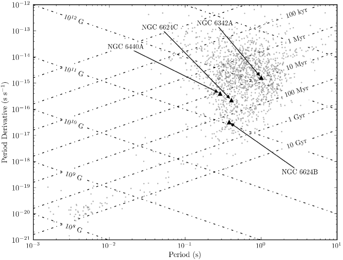
Figure 1: The $P$-$\dot{P}$ diagram showing the four NRPs in GCs as black triangles. The gray points are all Galactic pulsars from the ATNF Pulsar Database (Manchester et al., 2005). GC MSPs have been excluded because their $\dot{P}$s are usually contaminated by acceleration in the cluster potential. Lines of constant characteristic age and surface magnetic field are also plotted.

There are currently 144 pulsars known in 28 Galactic globular clusters (GCs). The vast majority of these are millisecond pulsars (MSPs), characterized by short spin periods and small period-derivatives. Such a population arises quite naturally in GCs, which are old stellar systems that are thought to contain a reservoir of primordial neutron stars (NSs) (Hut et al., 1992). In the dense environments in the cores of most GCs, these NSs undergo frequent exchange interactions, and may then be “recycled” into MSPs by accreting matter from a binary companion (Alpar et al., 1982). In addition to these MSPs, however, there is a small but enigmatic population of long-period pulsars that seem similar to the “normal” pulsars usually found in the Galactic disk (see Figure 1) (Biggs et al., 1994; Lyne et al., 1996; Chandler, 2003; Lynch et al., 2012). We will refer to these as non-recycled pulsars (NRPs) throughout this paper to distinguish them from the normal Galactic disk pulsars. The standard scenario for forming normal disk pulsars involves the core collapse of a massive star, giving rise to a young pulsar with a high magnetic field, which quickly spins down to $P\sim 0.3\;\textrm{s}$ (Faucher-Giguère & Kaspi, 2006). The inferred lifetimes of normal pulsars are typically $10$ to $100\;\textrm{Myr}$ (Ridley & Lorimer, 2010), and as such, they are usually associated with the recent death of massive stars, which themselves have lifetimes $\lesssim 100\;\textrm{Myr}$. This is where the mystery of NRPs in GCs arises—GCs are composed of old, $\lesssim 1\;\mathrm{M_{\sun}}$ stars, and all stars massive enough to form NSs (along with any pulsars that were formed) should have died some $\sim 10\;\textrm{Gyr}$ ago. The fact that several NRPs are observed in GCs requires an alternative to the standard core collapse model.

Several authors (Lyne et al., 1996; Ivanova et al., 2008) have invoked the collapse of a massive O-Ne-Mg white dwarf (WD) via electron capture (so called electron capture supernovae, or ECS (Nomoto, 1984, 1987)). Recent theoretical work supports the notion that ECS are essential for understanding the full population of neutron stars in GCs (Ivanova et al., 2008). Unfortunately, ECS have never been directly observed and their energetics remain uncertain, although there is good reason to believe that they are about an order of magnitude less energetic than core collapse supernovae (CCS) (Kitaura et al., 2006; Dessart et al., 2006). This probably leads to small natal kicks when combined with a faster and more symmetric explosion than in CCS (Podsiadlowski et al., 2004). NRPs may be an important observational constraint on the properties of ECS.

Motivated by the large number of recent and sensitive pulsar searches of GCs, Boyles et al. (2011, hereafter Paper i@) used statistical techniques to explore the underlying population of NRPs in GCs. The results are based solely on observations and some simplifying assumptions about the luminosity function and lifetime of NRPs, and as such provide a constraint on the birthrate of NRPs in GCs, regardless of how they are formed. One of the key results from this study was the compilation of probability distributions for the birthrates of NRPs in the majority of GCs.

Paper i@ gave detailed consideration only to those pulsars that gained a sufficiently small natal kick as to be retained by their host clusters. Given the high upper limits on the birthrate of GC NRPs and the relatively shallow potentials of most GCs, there is an intriguing possibility that a large population of NRPs may have escaped from their progenitor clusters at birth and entered the field of the Galaxy, where they could contribute to the observed population of normal disk pulsars. Building on the results of Paper i@, we have carried out Monte Carlo simulations to explore the properties of this purported population, and the feasibility of detecting it as a separate group. In §2 we provide a brief overview of the techniques and results from Paper i@. In §3 we describe our simulations and present the results in §4. We discuss the implications of these results in §5 and summarize in §6.

2 Overview of Paper i@

The goal of Paper i@ was to characterize the underlying population of NRPs in a cluster using observational constraints. Obviously, this approach is only valid for clusters that have been searched for pulsars. Paper i@ compiled results from searches of 97 clusters (out of 156 listed in Harris (2010)) carried out by numerous groups (see Paper i@ for a complete list and references). For each search, the detection probability was defined as

$$\theta(L_{\mathrm{min}},f(L))=\frac{\int_{L_{\mathrm{min}}}^{\infty}{f(L)\>dL}}{\int_{0}^{\infty}{f(L)\>dL}},$$ (1)

where $L_{\mathrm{min}}$ is the limiting luminosity of the search, and $f(L)$ is the luminosity distribution of NRPs. In words, $\theta$ is simply the fraction of pulsars that lie above $L_{\mathrm{min}}$. Five log-normal distributions with different parameters were used for $f(L)$; one given by Faucher-Giguère & Kaspi (2006) and four by Ridley & Lorimer (2010). This gave rise to a range of values for $\theta$.

Bayes’ theorem was then used to obtain a probability density function (PDF) for the total number of potentially observable NRPs ($N$), given the number of actual detections ($n$), and $\theta$. Potentially observable means all NRPs that currently reside in clusters and whose radio beams cross our line of sight (i.e., all those that could be observed with infinite sensitivity). We shall discuss corrections to this number in §3. This PDF is

$$\mathcal{P}(N,\theta|n)\propto\mathcal{L}(n,N|\theta)\mathcal{P}(N,\theta),$$ (2)

where $\mathcal{L}(n,N|\theta)$ is the likelihood of detecting $n$ pulsars from a population of $N$ given $\theta$, and $\mathcal{P}(N,\theta)$ is the joint prior PDF for $N$ and $\theta$. Since pulsar searches have only two possible outcomes (success or failure), Paper i@ chose the binomial distribution for the likelihood:

$$\mathcal{L}(n,N|\theta)=\frac{N!}{n!(N-n)!}\theta^{n}(1-\theta)^{N-n}.$$ (3)

To characterize the joint prior, $\mathcal{P}(N,\theta)$, Paper i@ first assumed that $N$ and $\theta$ were independent. The prior for $N$ was taken to be a uniform distribution on $[n,\infty)$, so that the only restriction is $N\geq n$. The prior for $\theta$ was also taken to be uniformly distributed on $[\theta_{\mathrm{min}},\theta_{\mathrm{max}}]$, where $\theta_{\mathrm{min}}$ and $\theta_{\mathrm{max}}$ correspond to the lowest and highest values of $\theta$ for different choices of $f(L)$. Having obtained $\mathcal{P}(N,\theta|n)$, Paper i@ then marginalized over $\theta$ to obtain a final PDF for $N$ (denoted as $\mathcal{P}(N|n)$) for each of the 97 clusters in the sample.

3 Simulating NRPs that Escape from Clusters

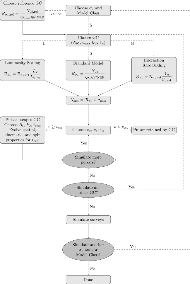
Figure 2: A schematic diagram describing our simulation strategy. The abbreviations for model classes are: S = standard models (no scaling); L = luminosity scaling; G = core interaction rate scaling.

As mentioned in §2, it is necessary to correct $\mathcal{P}(N|n)$ to account for the fraction of NRPs whose radio beams do not cross our line of sight, and for those who are no longer bound to their progenitor GCs. This second correction is necessary because GCs have fairly shallow potentials, with escape velocities $v_{\mathrm{esc}}\sim 30\;\textrm{km}\,\mathrm{s^{-1}}$. Some NRPs will inevitably escape the cluster due to the natal kicks they receive during formation and enter the field of the Galaxy. This is precisely the population that we are interested in here. We have used Monte Carlo simulations to model the evolution of NRPs that escaped from GCs and to determine if this population could be distinguished observationally from other pulsars in the Galaxy. We proceed in four steps: i) we determine the number of NRPs that will enter the Galaxy; ii) we model the spatial and kinematical evolution of this population; iii) we model the rotational and electromagnetic evolution; and iv) we “detect” this evolved population by simulating a number of large-area pulsar surveys. As described in the following sections, we actually explore several different types of models for the population, and for each model we also explore several natal kick distributions. To ensure robust statistical results, each combination of model class and kick distribution is simulated ten times, and the final results are taken to be the mean of these runs. Figure 2 is a schematic overview of our simulations. We discuss each step below.

3.1 Determining the Number of Escaped NRPs

We choose to characterize $\mathcal{P}(N|n)$ by the upper bound of the 95% confidence interval, which we denote as $N_{95}$ (note that the birth rates discussed in Paper i@ used the median of this distribution). This is corrected for beaming and escaping pulsars, and divided by the mean lifetime of NRPs to obtain a birth rate for each cluster that we consider,

$$\mathcal{R}_{\sigma_{v}}=\frac{N_{95}}{\eta_{\mathrm{beam}}\eta_{\sigma_{v}}\tau_{\mathrm{NRP}}},$$ (4)

where $\mathcal{R}_{\sigma_{v}}$ is the birth rate, $\eta_{\mathrm{beam}}=0.1$ is the beaming fraction (Tauris & Manchester, 1998), $\eta_{\sigma_{v}}$ is the correction for escaping pulsars, and $\tau_{\mathrm{NRP}}$ is the average pulsar lifetime. We derive an average lifetime of $43\;\textrm{Myr}$ by taking the total number of radio-loud pulsars ($1.2\times 10^{6}$) and dividing it by the Galactic pulsar birthrate ($2.8\;\mathrm{century}^{-1}$) (Faucher-Giguère & Kaspi, 2006). The subscript $\sigma_{v}$ refers to the mean birth velocity dispersion. The actual value of $\sigma_{v}$ for NRPs is unknown, since they are probably not formed via typical CCSNe , so we vary this parameter in our simulations. As we shall see, there is good reason to believe $\sigma_{v}\sim 10\;\textrm{km}\,\mathrm{s^{-1}}$. We assume that birth velocities can be described by a Maxwell-Boltzmann distribution so that the fraction of NRPs with $v\leq v_{\mathrm{esc}}$ is

$$\eta_{\sigma_{v}} = \frac{\int_{0}^{v_{\mathrm{esc}}}{f_{\mathrm{MB}}(v)\>dv}}{\int_{0}^{\infty}{f_{\mathrm{MB}}(v)\>dv}}$$

$$= \mathrm{erf}\left(\frac{v_{\mathrm{esc}}}{\sqrt{2\sigma_{v}}}\right)-\sqrt{\frac{2}{\pi}}\frac{v_{\mathrm{esc}}}{\sigma_{v}}\>\exp{\left(\frac{-v_{\mathrm{esc}}^{2}}{2\sigma_{v}^{2}}\right)},$$ (5)

where $f_{\mathrm{MB}}(v)$ is the Maxwell-Boltzmann distribution and $\mathrm{erf}$ signifies the error function

$$\mathrm{erf}(x)=\frac{2}{\sqrt{\pi}}\int_{0}^{x}e^{-t^{2}}\>dt$$ (6)

Escape velocities for each cluster were taken from Gnedin et al. (2002). For clusters without a reported value, we assumed $v_{\mathrm{esc}}=30\;\textrm{km}\,\mathrm{s^{-1}}$, which is roughly the median value from Gnedin et al. (2002).

Having obtained $\mathcal{R}_{\sigma_{v}}$, all that remains is to choose a time scale, $\tau_{\mathrm{max}}$, over which we will consider the evolution of this population. The number of pulsars to simulate per cluster then becomes $N_{\mathrm{sim}}=\mathcal{R}_{\sigma_{v}}\times\tau_{\mathrm{max}}$. In our simulations, we choose $\tau_{\mathrm{max}}=200\;\textrm{Myr}$. As we explain in §3.3, many pulsars will cease radio emission on timescales shorter than this. We choose a large value for $\tau_{\mathrm{max}}$ to ensure that we treat long-lived NRPs properly.

We refer to the above approach as our “standard model” (hereafter Sa). $N_{\mathrm{sim}}$ is obtained directly from the results of Paper i@, which is to say, without using any information about the clusters except for their escape velocities. However, the value of $N_{95}$, and hence $N_{\mathrm{sim}}$, depends heavily on $L_{\mathrm{min}}$, in the sense that $N_{95}$ will be larger (and not very constraining) for shallowly searched GCs. Therefore, we included three refinements to Sa in our study.

The first we call the “modified standard model” (Sb). For this, we simply exclude 16 clusters with $L_{\mathrm{1.4\;GHz,min}}\geq 7.5\;\textrm{mJy}\,\textrm{kpc}^{2}$, which reduces the number of shallowly searched clusters with very high values of $N_{95}$. While this sensitivity cut-off is somewhat arbitrary, it strikes a good balance between keeping enough clusters for the simulations to have meaningful results, while preventing unwieldy computations due to extremely large numbers of simulated escaping NRPs.

In the next two models, we choose a reference cluster, and scale all other values of $N_{\mathrm{sim}}$ by some chosen parameter. We use M22 as a reference cluster because it has the lowest value of $L_{\mathrm{min}}$ and consequently the most tightly constrained $N_{\mathrm{sim}}$ (relevant parameters of M22 can be found in Table 1). In the first approach, we scale by the V-band luminosity of each cluster, $L_{\mathrm{V}}$, so that

$$N^{\mathrm{L}}_{\mathrm{sim}}=N_{\mathrm{sim,M22}}\frac{L_{\mathrm{V}}}{L_{\mathrm{V,M22}}}.$$ (7)

This is the “luminosity scaling model” (L). Our reasoning is that at the very least, the number of NRPs produced in a cluster should scale with the number of progenitors in the cluster. However, to determine the number of progenitors would require first identifying those progenitors, and then making some assumptions about how their number scales with other properties of the cluster. We sought a more general approach, hence our decision to use the luminosity of the cluster—brighter clusters should be more massive (to within a factor of the cluster’s mass-to-light ratio), and more massive clusters should contain more NRP progenitors. Furthermore, the V-band luminosity is fairly easily determined as long as the distance to the cluster and reddening effects are well constrained, and is also readily available for nearly all Milky Way GCs.

Finally, we also scale by the so-called core interaction rate, $\Gamma_{\mathrm{c}}\propto\rho_{\mathrm{c}}^{1.5}r_{\mathrm{c}}^{2}$, where $\rho_{\mathrm{c}}$ is the central density of the cluster and $r_{\mathrm{c}}$ is the core radius; thus we have

$$N^{\mathrm{G}}_{\mathrm{sim}}=N_{\mathrm{sim,M22}}\frac{\Gamma_{\mathrm{c}}}{\Gamma_{\mathrm{c,M22}}}.$$ (8)

We call these the “interaction rate scaling models” (G). $\Gamma_{\mathrm{c}}$ has been shown to correlate well with the number of low-mass X-ray binaries and MSPs in a cluster (Pooley et al., 2003; Abdo et al., 2010), further supporting the notion that both populations are related to binary exchange interactions. A leading explanation for NRPs in GCs are ECS, particularly via accretion or merger induced collapse. These scenarios also require mass-transfer or merger in a binary system. Hence, it is interesting to explore models in which NRPs also have some dependence on $\Gamma_{\mathrm{c}}$.

For each of these models, relevant parameters ($N95$, $L_{\mathrm{V}}$, and $\Gamma_{\mathrm{c}}$) were only available for a subset of all 156 Milky Way GCs. It will be necessary to adjust our final results to account for unmodeled clusters, but we save this step for §4. Table 2 summarizes each class of models.

3.2 Spatial and Kinematical Evolution

In this step, we model the evolution of the escaping NRPs as they travel through the Galaxy. We begin by defining a Galactocentric coordinate system with

$$x = D\cos{b}\sin{\ell},$$ (9)

$$y = D_{\sun}-D\cos{b}\cos{\ell},\mathrm{~{}and}$$ (10)

$$z = D\sin{b}$$ (11)

where $D$ is the distance, $D_{\sun}=8.5\;\textrm{kpc}$ is the Sun’s distance from the Galactic center, $b$ is Galactic latitude, and $\ell$ is Galactic longitude. Note that this differs from the typical Cartesian Galactic coordinates, where it is usually the $x$-axis that connects the Sun and Galactic center. This was done for compatibility with previously developed software tools.

We assign each NRP initial coordinates that are equal to the coordinates of the host GC. Initial 3-D velocity components ($v_{x,\mathrm{i}}$, $v_{y,\mathrm{i}}$, $v_{z,\mathrm{i}}$) are chosen at random from a normal distribution with a zero mean and standard deviation of $\sigma_{v}$ (this is equivalent to a Maxwell-Boltzmann distribution for the full space velocity). If the total space velocity with respect to the GC, $v_{\mathrm{i}}=(v_{x,\mathrm{i}}^{2}+v_{y,\mathrm{i}}^{2}+v_{z,\mathrm{i}}^{2})^{1/2}\geq v_{\mathrm{esc}}$, then we consider the pulsar to have escaped from its host cluster and entered the field of the Galaxy. Although we keep track of the number of pulsars retained by their host clusters, we do not consider them further. All subsequent analysis on the number of emiting and detectable NRPs deals only with those that escape. We treat each GC as being fixed at its current position in the Galaxy. In reality, the clusters are on their own orbits, and the pulsars will inherit the systemic velocity of their progenitor clusters. Each pulsars enters the field of the Galaxy with $v_{\mathrm{field}}=(v_{\mathrm{i}}^{2}-v_{\mathrm{esc}}^{2})^{1/2}$.

Having chosen initial spatial and velocity components, we integrate the motion of each pulsar through the Galactic potential. Following Carlberg & Innanen (1987) and Kuijken & Gilmore (1989) (see also Wex et al., 2000), we use a 3-component Galactic potential of the form

$$\phi^{i}(R,Z)=-GM^{i}\left[\left(a^{i}+\sum\limits_{j=1}^{3}\left[\beta_{j}^{i}\sqrt{Z^{2}+h_{j}^{i}}\,\right]\right)^{2}+b^{i}+R^{2}\right]^{-1/2},$$ (12)

where the superscript $i=\mathrm{D,B,N}$ indicates the contribution from the disk-halo, bulge, or nucleus, respectively. The full potential is the sum of these three components. The values of $M^{i}$, $a^{i}$, $b^{i}$, $\beta^{i}_{j}$, and $h^{i}_{j}$ can be found in Table 3. The integration time, $t_{\mathrm{evol}}$, is chosen at random from a uniform distribution on the interval $[0,200\;\textrm{Myr}]$. In other words, we assume that an NRP may be born at any point in the past $200\;\textrm{Myr}$, and evolve it forward to the present. This also assumes that the birthrate of NRPs is constant over this interval. The final spatial and kinematical properties are then recorded for later analysis.

3.3 Rotational Evolution and Energetics

Birth spin periods and surface magnetic fields ($B_{\mathrm{s}}$) are chosen at random for each escaping NRP. Following Faucher-Giguère & Kaspi (2006), we use a normal distribution for $P_{0}$ with a mean of $0.3\;\textrm{s}$ and standard deviation of $0.15\;\textrm{s}$. Negative periods are rejected and redrawn. We also use a log-normal distribution for $B_{\mathrm{s}}$, with a mean in the base-10 logarithm of $12.65$ and standard deviation $0.55$.

We evolve the pulsar’s rotation under the assumption of pure magnetic dipole braking and a constant magnetic field, so that the observed period and period derivative are

$$P = \left(\frac{P_{0}^{2}+16\pi B_{\mathrm{s}}^{2}R^{6}t_{\mathrm{evol}}}{3c^{3}I}\right)^{1/2}\mathrm{~{}and}$$ (13)

$$\dot{P} = \frac{P^{2}-P_{0}^{2}}{2Pt_{\mathrm{evol}}},$$ (14)

where $R=10\;\textrm{km}$ and $I=10^{45}\;\textrm{gm}\,\mathrm{cm^{2}}$ are the assumed radius and moment of inertia for the pulsar, respectively, and $t_{\mathrm{evol}}$ is defined as above. Hence, we arrive at the final $P$ and $\dot{P}$ at the end of our simulation.

We calculate the observed luminosity using a power-law model that depends on $P$ and $\dot{P}$. We prefer this model because it relates the luminosity to the rotational energy loss of the pulsar. Once again, we turn to Faucher-Giguère & Kaspi (2006) for the exact form of this power-law:

$$L=10^{L_{\mathrm{cor}}}L_{0}P^{-3/2}\left(\frac{\dot{P}}{10^{-15}\;\textrm{s}\,\mathrm{s^{-1}}}\right)^{1/2}.$$ (15)

$L_{0}=0.18\;\textrm{mJy}\,\textrm{kpc}^{2}$ is a “standard” luminosity and $L_{\mathrm{cor}}$ is a correction factor that accounts for uncertainty in the model. It is drawn at random from a normal distribution with zero mean and standard deviation $\sigma_{L_{\mathrm{cor}}}=0.8$.

Pulsars have finite lifetimes, and at some point will cease radio emission. This seems to correspond to a “death-line” in the $P$-$\dot{P}$ diagram, which is well described theoretically (Bhattacharya et al., 1992) and empirically as

$$\frac{B_{\mathrm{s}}}{P^{2}}=1.7\times 10^{11}\;\textrm{G}\,\mathrm{s^{-2}}.$$ (16)

Any pulsars with $B_{\mathrm{s}}P^{-2}$ less than this value will no longer be visible. We track the evolution of these pulsars, but do not include them for consideration in the next step.

3.4 Simulated Surveys

The final step is to “search” for potentially visible NRPs by simulating various large-area surveys. A pulsar can be detected only if its signal-to-noise ratio (S/N) lies above the minimum S/N threshold of a given survey. Following Lorimer & Kramer (2004),

$$\textrm{S/N}=S_{\nu}\frac{G\sqrt{N_{\mathrm{pol}}\Delta\nu t_{\mathrm{int}}}}{\beta(T_{\mathrm{sys}}+T_{\mathrm{sky}})}\sqrt{\frac{P}{W}-1}$$ (17)

where $S_{\nu}$ is the flux density of the pulsar, $G$ is the telescope gain, $N_{\mathrm{pol}}$ is the number of summed polarizations, $\Delta\nu$ is the bandwidth, $t_{\mathrm{int}}$ is the integration time, $\beta$ is a factor that accounts for quantization losses, $T_{\mathrm{sys}}$ and $T_{\mathrm{sky}}$ are the system and sky temperatures, respectively, and $W$ is the observed pulse width. Most of these factors are intrinsic to the specific survey in question, but $T_{\mathrm{sky}}$ and $W$ depend on the position and properties of the pulsar. Sky temperatures at the position of each pulsar are taken from the $408\;\textrm{MHz}$ survey of Haslam et al. (1982) and scaled to the appropriate frequency assuming a power-law with a spectral index of $-2.6$. The pulse width is described as the quadrature sum of

$$W^{2}=W_{\mathrm{int}}^{2}+t_{\mathrm{samp}}^{2}+t_{\mathrm{DM}}^{2}+\tau_{\mathrm{s}}^{2},$$ (18)

where $W_{\mathrm{int}}$ is the intrinsic pulse width, $t_{\mathrm{samp}}$ is the instrumental sampling time, $t_{\mathrm{DM}}$ is the dispersive smearing within a given frequency channel, and $\tau_{\mathrm{s}}$ is the scattering time. We model the intrinsic width as

$$\log{W_{\mathrm{int}}}=\log{\left[0.06\left(\frac{P}{\textrm{ms}}\right)^{0.9}\right]}+\varsigma,$$ (19)

where $\varsigma$ is a random variable drawn from a normal distribution with a standard deviation of $0.3$ (Lorimer et al., 2006). The sampling time for each survey is listed in Table 4. The dispersion measure (DM) is calculated using the known distance to the pulsar and the NE2001 model of Galactic free electron density (Cordes & Lazio, 2002). The dispersive smearing is then simply

$$t_{\mathrm{DM}}\simeq 8.3\times 10^{3}\;\textrm{s}\left(\frac{\textrm{DM}}{\mathrm{pc\;cm^{-3}}}\right)\left(\frac{\Delta\nu_{\mathrm{chan}}}{\textrm{MHz}}\right)\left(\frac{\nu}{\textrm{MHz}}\right)^{-3},$$ (20)

where $\Delta\nu_{\mathrm{chan}}$ is the channel width and $\nu$ is the center frequency (Lorimer & Kramer, 2004). Various empirical relations between $\tau_{\mathrm{s}}$ and DM appear in the literature. We use the relationship given by Cordes (2002):

$$\log{\left(\frac{\tau_{\mathrm{s}}}{\mathrm{\mu s}}\right)}=$$ (21)

$$-3.59+0.129\log{\left(\frac{\textrm{DM}}{\mathrm{pc\;cm^{-3}}}\right)}+1.02\left[\log{\left(\frac{\textrm{DM}}{\mathrm{pc\;cm^{-3}}}\right)}\right]^{2}-4.4\log{\left(\frac{\nu}{\textrm{GHz}}\right)}.$$

One factor that we do not model here is the affect of radio frequency interference (RFI), which can be particularly problematic for blind searches of long-period pulsars. Obviously, some surveys will be more affected by RFI because of proximity to man-made sources and/or poor instrumental resistance to strong RFI. Nonetheless, careful data analysis can help to mitigate these effects.

After determining the relevant parameters for each NRP, we use the survey tool from the psrpop software package (Lorimer et al., 2006) to simulate the surveys. Pulsar luminosities are scaled to the appropriate frequency assuming a power-law spectral index of $-1.6$.

We simulate five surveys: the Parkes Multibeam Survey (PMSURV) (Lorimer et al., 2006); the P-ALFA survey (Cordes et al., 2006), the GBT North Celestial Cap Survey (GBNCC); a visible-sky GBT survey similar to the GBNCC survey (GBTALL); and a hypothetical all-sky survey using a future Square Kilometer Array (SKA) (Smits et al., 2009). The characteristics of each survey can be found in Table 4. Each survey is simulated 100 times, for each run of the simulation, allowing us to characterize the median number of detected pulsars. Because the spatial, kinematical, and rotational evolution of the NRPs is simulated ten times for each combination of model class and $\sigma_{v}$ (see above), we have ten values for the median number of detected pulsars from each combination. The final reported number of detected NRPs ($N_{\mathrm{det}}$) is the mean of these ten values plus the standard error, and represents an upper limit.

4 Results

The results of our simulations can be found in Table 5. The values reported here have been multiplied by a scale factor ($156/N_{\mathrm{GC}}$) that accounts for clusters not included in that model class. This is equivalent to assuming that un-modeled clusters follow the average results for that model class. The total number of all NRPs that escape from their progenitor clusters ($N_{\mathrm{esc}}$) and that are retained by their host clusters ($N_{\mathrm{ret}}$) are listed in the first two columns. These include pulsars whose radio beams do not cross our line of sight as well as those that have crossed the death line; these will be dealt with in §4.2. Hence, these numbers represent 95% confidence interval upper limits on the total number of NRPs formed in the last $200\;\textrm{Myr}$.

It is immediately obvious that, for a given model class, $N_{\mathrm{esc}}$ increases with increasing $\sigma_{v}$. This is not at all surprising, since a larger kick velocity dispersion will lead to more high velocity pulsars that can escape the cluster potential. In contrast, $N_{\mathrm{ret}}$ remains nearly constant with $\sigma_{v}$. This is because we have essentially normalized all values by the “observable” (i.e., based on observations) value of $N_{95}$, which characterizes the number of retained NRPs. We point out that $\mathcal{R}_{\sigma_{v}}$ also increases with $\sigma_{v}$, so that there are more pulsars in total simulated for higher velocity dispersions. Model class Sa gives rise to the largest total number of NRPs by far. This is entirely due to the very high values of $N_{95}$ for most GCs. Even when we exclude the most unconstraining clusters from consideration in model class Sb, the total number of NRPs is still very large. Model class G produces fewer pulsars than Sb, while model class L produces the fewest of all. As we shall see in §5.1, this has important consequences for the viability of ECS as an explanation for NRPs. For now, we turn our attention to exploring the characteristics of the escaped population in more detail.

4.1 Spatial and Kinematical Properties

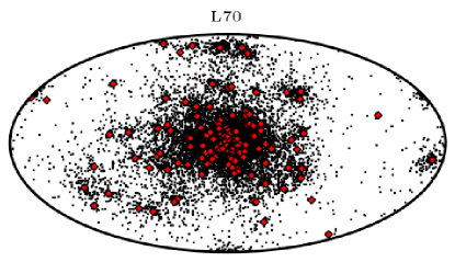
Figure 3: The position of all escaped pulsars in Galactic coordinates (as viewed from Earth) for model L70. Other models have a similar spatial distribution of pulsars but with varying numbers. The Galactic center is at the center of the plot. Globular clusters are represented by red diamonds, while pulsars are shown as black dots.

Figure 3 shows a sample sky distribution of all escaping NRPs for model L70 in Galactic coordinates (other models have very similar forms with different numbers of pulsars). The pulsars tend to group around their progenitor clusters. In models with higher $\sigma_{v}$ the pulsars travel further from their host clusters, as expected, but there are also more pulsars in total.

We also model calculate the proper motion of each pulsar. The proper motions are a combination of the kick velocity of the pulsar (evolved as the pulsar travles through the Galaxy) and the systemic velocity of the GC itself (both projected onto the plane of the sky). Pulsars from a common progenitor cluster will thus have similar systemic velocity components. The velocities of many GCs arepdf observed to be $\sim 100\;\textrm{km}\,\mathrm{s^{-1}}$, larger than the kick velocities received by the NRPs at birth.

4.2 Number of Detectable NRPs in Surveys

The results of our simulated surveys can be found in Table 5. It is at this stage that we account for pulsars that have crossed the death line. The third column gives the number of all radio emitting pulsars ($N_{\mathrm{emit}}$). The number of detected pulsars for various surveys is given in the following columns. These numbers have already been multiplied by a constant $\eta_{\mathrm{beam}}=0.1$ to account for pulsars whose radio beams do not cross our line of sight. It is immediately obvious that significant numbers of GC NRPs are detected only when $N_{\mathrm{emit}}$ is large (corresponding to large $\sigma_{v}$). The most successful survey is, not surprisingly, our hypothetical all-sky SKA survey. Such a survey would presumably be designed to detect nearly all potentially observable disk pulsars in the Galaxy, but only $\sim 8\%$ of emitting GC NRPs are detected. The next most promising survey is the hypothetical GBTALL, but this detects only $\sim 0.03\%$ of emitting NRPs. The success of the PMSURV and P-ALFA are less than but comparable to the GBTALL. The GBNCC detects very few, if any, NRPs. We can attribute this to the design of the survey, whose goal it is to find nearby and bright MSPs; the $1374\;\textrm{MHz}$ limiting flux density is an order of magnitude higher than PMSURV, P-ALFA, or the SKA survey. However, the GBTALL has an identical set-up and does much better. We attribute this to the large survey area and better coverage at low declinations, where most GCs are found. The PMSURV and P-ALFA both utilize high observing frequencies and long integration times to search for highly dispersed, and thus generally more distant pulsars. At first glance it may seem strange that so few NRPs are detected, given that we already know of four that reside in GCs. These pulsars were detected in targeted surveys with very long integration times. Furthermore, for low $\sigma_{v}$, we predict $N_{\mathrm{esc}}<N_{\mathrm{ret}}$; in models where $N_{\mathrm{esc}}\approx N_{\mathrm{ret}}$, the number of detected NRPs is closer to what is actually observed in clusters.

We can conclude that, to have any hope of detecting large numbers of escaped NRPs, surveys must be very sensitive and cover as much sky as possible. Even then, success will depend strongly on the size of the underlying population, which depends on the kick velocity of NRPs.

5 Discussion

5.1 Which Models are Realistic?

One of the primary findings of Paper i@ was that very high values of $\sigma_{v}$ greatly overproduce NRPs in GCs according to any reasonable metric. For example, they find a birth rate of $422$ and $0.25\;\mathrm{psr\,century^{-1}}$ for $\sigma_{v}=130$ and $10\;\textrm{km}\,\mathrm{s^{-1}}$, respectively (keep in mind that these are for the median number of NRPs, whereas we use the higher 95% confidence upper limit). For comparison, the birth rate of normal disk pulsars is $2.8\;\mathrm{psr\,century^{-1}}$ (Faucher-Giguère & Kaspi, 2006). More relevant for the case of NRPs is how these results compare with the population of WDs that are the likely progenitors to NRPs via ECS. Paper i@ estimated the total number of WDs that could potentially form NSs via ECS to be $\sim 2.1\times 10^{5}$ across the entire GC population. If we assume that all of these WDs eventually become NSs and that the birthrate of NRPs is constant, then the timescale for exhausting this population is simply $2.4\times 10^{5}/\mathcal{R}_{\sigma_{v}}$. These timescales, $\tau_{\mathrm{exhaust}}$, are given for each of our models in Table 6. Even for the smallest $\mathcal{R}_{\sigma_{v}}$ in our standard models, $\tau_{\mathrm{exhaust}}\lesssim 100\;\textrm{Myr}$. This is only $\sim 1\%$ the age of a typical GC ($\sim 10\;\textrm{Gyr}$). Although these birth rates are only upper limits, such a large discrepancy seems difficult to explain. Recall, however, that our standard models are heavily affected by the limiting luminosity of cluster searches, so we believe that these results simply indicate that the standard models are not very well constrained. Model class G, where we scale the number of NRPs formed in M22 by the core interaction rate of a cluster, produces fewer NRPs than our standard models. Nonetheless, inspection of Table 6 indicates that the implied birthrates are still probably too high.

However, the situation improves for model class L, where we scale by the luminosity of a cluster. High velocity dispersion cases still seem to overproduce the number of NRPs considerably, but for $\sigma_{v}<30\;\textrm{km}\,\mathrm{s^{-1}}$ the implied birth rates are low enough that the resevoir of WDs may last for $>15\%$ of the age of the typical cluster. When one considers that the birth rates reported here are only 95% confidence upper limits, it seems that ECS are a viable explanation for NRPs after all. Given that the true efficiency in going from WDs to NRPs is probably $<100\%$, we favor a typical ECS kick velocity of $\lesssim 10\;\textrm{km}\,\mathrm{s^{-1}}$. Other authors have inferred small $\sigma_{v}$ for ECS as well. Pfahl et al. (2002) studied the eccentricities of high-mass X-ray binaries that are believed to form via ECS and concluded that $\sigma_{v}\lesssim 50\;\textrm{km}\,\mathrm{s^{-1}}$. More recently, Martin et al. (2009) used a similar line of reasoning to argue for $\sigma_{v}\sim 15\;\textrm{km}\,\mathrm{s^{-1}}$ (though the authors note that this may be in conflict with the observed misalignment between the rotational and orbital spin axes in these systems). PSR J0737$-$3039B is also believed to have formed via ECS (Podsiadlowski et al., 2005) and Wong et al. (2010) find a 95% confidence interval of $5$–$120\;\textrm{km}\,\mathrm{s^{-1}}$ for the kick of this neutron star. Our results are in general agreement with the notion that ECS must be less energetic and lead to smaller neutron star kicks than CCS, but may be more constraining than other estimates.

With a firm estimate of the efficiency for converting WDs to NRPs and the duration of this process, a more exact estimate could be made. There are two important caveats to keep in mind, however. The first is that model classes L and G are based on the upper limit of the number of NRPs in only one cluster, M22. We chose this cluster because it has been searched to a lower limiting luminosity than any other. If M22 is an atypical cluster in terms of its NRP content, then this would bias our results. However, other clusters (e.g. M28, 47 Tucanae, Terzan 5) have been deeply searched and also have small implied NRP birth rates. Model classes L and G also assume that only one characteristic of a GC influences the number of NRPs that are formed. Paper i@ found evidence suggesting that metallicity may play a significant role in the formation of NRPs, and we cannot rule out other factors.

The best way to differentiate between these results and those presented in Paper i@ would be to search a large number of GCs more deeply. This would yield much tighter constraints for the method used in Paper i@, and would reduce the number of simplifying assumptions we need to make here.

5.2 Can the Population of Escaped NRPs Be Identified?

The next question to ask is, what are the prospects for identifying the population of escaped NRPs as separate from normal disk pulsars? In the following discussion, we will limit ourselves to the results for model class L. With large numbers of pulsars it may be able to identify NRPs based on their spatial distribution around GCs or their kinematic similarities, since NRPs born from the same GC should have the same systemic contributions to their velocities. Unfortunately, we favor models with low $\sigma_{v}$, and as §4.2 makes clear, in this case even the best surveys can detect $\lesssim 100$ NRPs. Proper motions would probably only be available on a sub-set of these pulsars. However, when the SKA comes online, it will be able to measure proper motions interferometricaly on nearly all pulsars it detects, so this may be a future avenue for obtaining proper motions. Nonetheless, it is worth keeping our results in mind as high sensitivity surveys are carried out.

Large area surveys are not the only means by which GC NRPs could be detected. Since many escaped NRPs are found to remain fairly close to their progenitor clusters, especially for our favored low $\sigma_{v}$ models, targeted surveys of the regions around GCs could be more fruitful, as it would allow for deeper integrations and better sensitivity. We have calculated the minimum distance between an escaped NRP and a GC for all emitting pulsars in our simulation. There is some dependence on $\sigma_{v}$, but in general $\sim 3$–$7\%$, $\sim 13$–$16\%$, and $\sim 20$–$25\%$ of NRPs lie within $1^{\circ}$, $3^{\circ}$, and $5^{\circ}$ of a GC, respectively. However, a large $\sigma_{v}$ would still give rise to a larger pool of potentially observable pulsars. A survey covering a $\sim 3^{\circ}$ radius around all GCs would then, in principle, capture roughly $15\%$ of the population of NRPs. However, with 156 Milky Way GCs, this would amounts to a total survey area of over 4400 square degrees, with each portion requiring substantial integration times. Such a survey would be very difficult. The situation is improved if such a survey were limited to only $1^{\circ}$ around each cluster (reducing the survey area to about 500 square degrees) or by targeting only the most promising GCs, such as those already known to contain an NRP, but this would also decrease the likely number of NRPs that could be detected.

6 Conclusions

Paper i@ explored the enigmatic population of NRPs found in GCs by setting limits on the size of the population using the results of various GC surveys. We have built upon these results to explore the properties of NRPs that escape from clusters and enter the field of the Galaxy. We agree with Paper i@ that current GC surveys are not sensitive enough to constrain the population on their own. However, if we assume that the number of NRPs in a GC scale with some properties of the cluster, specifically luminosity (as a proxy for cluster mass), then the size of the population is more realistic. It seems that in these cases, ECS may be sufficient to account for GC NRPs. We favor models that rely on luminosity scaling and invoke a low natal kick velocity ($\sim 10\;\textrm{km}\,\mathrm{s^{-1}}$), but there is still too much uncertainty in how NRPs are formed to place more definite limits. Unfortunately, large numbers of escaped NRPs would be difficult to detect with any current large-area pulsar surveys, so the chances of identifying them as a separate population are slim. The best prospects lie with future surveys with the SKA. If sufficiently large numbers of GC NRPs can be detected in the field of the Galaxy, it may be possible to distinguish them from normal disk pulsars through their spatial distribution and proper motions. The best approach for learning more about NRPs, though, remains identifying those that are bound to their progenitor GCs. This will require more sensitive searches of many clusters.

We are extremely grateful to Norbert Wex for providing us with an independent method for checking the results of our simulations. We thank an anonymous referee for reviewing this manuscript. We would also like to thank the National Science Foundation for supporting this work through grant AST-0907967. The National Radio Astronomy Observatory is a facility of the National Science Foundation operated under cooperative agreement by Associated Universities, Inc.

Table 1: Properties of M22 Used for Scaling

$N_{95}$	$v_{\mathrm{esc}}$	$L_{\mathrm{V}}$	$\log{\rho_{\mathrm{c}}}$	$r_{\mathrm{c}}$
	($\textrm{km}\,\mathrm{s^{-1}}$)	($L_{\mathrm{\sun,V}}$)	($\mathrm{L_{\sun}}\,\mathrm{pc^{-3}})$	(pc)
4	44.7	$2.15\times 10^{5}$	3.63	1.2

Note. — Structural parameters have been taken from Harris (2010), and we have used $D=3.2\;\textrm{kpc}$ for calculating $r_{c}$ in physical units. The escape velocity is from Gnedin et al. (2002).

Table 2: Summary of Models Used to Simulate the Population of NRPs

Model Class	$N_{\mathrm{GC}}$	Scaling
Sa	97	None
Sb	81	None
L	156	Luminosity
G	143	$\Gamma_{\mathrm{c}}$

Note. — Ten runs were performed for each value of $\sigma_{v}$ for each model class.

Table 3: Parameters Used in the Model of Galactic Potential

Component	$M$	$a$	$b$	$\beta_{1}$	$h_{1}$	$\beta_{2}$	$h_{2}$	$\beta_{3}$	$h_{3}$
	($10^{9}\;\mathrm{M_{\sun}}$)	(kpc)	(kpc)		(kpc)		(kpc)		(kpc)
Disk-Halo	145	2.4	5.5	0.4	0.325	0.5	0.090	0.1	0.125
Bulge	9.3	0	0.25	1	0	0	0	0	0
Nucleus	10	0	1.5	1	0	0	0	0	0

Note. — See §3.2 for parameter definitions.

Table 4: Large-area Survey Parameters

Survey	$f_{\mathrm{sky}}$	$G$	$T_{\mathrm{sys}}$	$\nu_{\mathrm{obs}}$	$\Delta\nu$	$t_{\mathrm{samp}}$	$t_{\mathrm{int}}$	$\beta$	$S_{\mathrm{1374\;MHz,min}}$
	(%)	($\textrm{K}\;\textrm{Jy}^{-1}$)	(K)	(MHz)	(MHz)	($\mathrm{\mu s}$)	(s)		($\mathrm{\mu Jy}$)
PMSURV	4.6	0.6	25	1374	288	250	2100	1.2	160
P-ALFA	10.9	8.5	25	1374	300	64	268	1.1	100
GBNCC	19.2	2.0	46	350	100	81.92	120	1.1	2000
GBTALL	86.0	2.0	46	350	100	81.92	120	1.1	2000
SKA	100	140	25	1374	512	50	2100	1.0	0.45

Note. — All surveys use two summed polarizations.

Table 5: Simulation Results

Model ID	$N_{\mathrm{esc}}$	$N_{\mathrm{ret}}$	$N_{\mathrm{emit}}$	$N_{\mathrm{det}}$
				PMSURV	PALAFA	GBNCC	GBTALL	SKA
Sa5	$1.3\times 10^{6}$	$9.5\times 10^{5}$	$1.5\times 10^{5}$	$3$	$0$	$0$	$83$	$1.1\times 10^{4}$
Sa10	$1.0\times 10^{7}$	$9.5\times 10^{5}$	$1.2\times 10^{6}$	$40$	$6$	$0$	$2.6\times 10^{2}$	$9.2\times 10^{4}$
Sa20	$8.0\times 10^{7}$	$9.7\times 10^{5}$	$9.1\times 10^{6}$	$3.9\times 10^{2}$	$51$	$0$	$3.5\times 10^{3}$	$6.9\times 10^{5}$
Sa30	$2.7\times 10^{8}$	$1.0\times 10^{6}$	$3.1\times 10^{7}$	$3.0\times 10^{2}$	$7.0\times 10^{2}$	$0$	$7.9\times 10^{3}$	$2.4\times 10^{6}$
Sa50	$1.2\times 10^{9}$	$9.2\times 10^{5}$	$1.4\times 10^{8}$	$5.4\times 10^{3}$	$5.9\times 10^{2}$	$0$	$5.4\times 10^{4}$	$1.1\times 10^{7}$
Sa70	$3.4\times 10^{9}$	$9.7\times 10^{5}$	$4.2\times 10^{8}$	$1.0\times 10^{4}$	$2.4\times 10^{3}$	$1$	$1.1\times 10^{5}$	$3.0\times 10^{7}$
Sa100	$9.9\times 10^{9}$	$9.3\times 10^{5}$	$1.1\times 10^{9}$	$6.1\times 10^{4}$	$5.4\times 10^{3}$	$35$	$3.7\times 10^{5}$	$8.3\times 10^{7}$
Sb5	$3.4\times 10^{4}$	$4.7\times 10^{5}$	$3.5\times 10^{3}$	$0$	$0$	$0$	$2$	$3.8\times 10^{2}$
Sb10	$3.8\times 10^{5}$	$4.8\times 10^{5}$	$3.6\times 10^{4}$	$6$	$6$	$0$	$23$	$4.3\times 10^{3}$
Sb20	$3.3\times 10^{6}$	$4.9\times 10^{5}$	$3.3\times 10^{5}$	$63$	$62$	$0$	$2.1\times 10^{2}$	$3.8\times 10^{4}$
Sb30	$1.1\times 10^{7}$	$5.1\times 10^{5}$	$1.1\times 10^{6}$	$2.5\times 10^{2}$	$1.9\times 10^{2}$	$0$	$5.0\times 10^{2}$	$1.3\times 10^{5}$
Sb50	$5.2\times 10^{7}$	$5.2\times 10^{5}$	$4.9\times 10^{6}$	$9.0\times 10^{2}$	$7.2\times 10^{2}$	$0$	$2.4\times 10^{3}$	$5.8\times 10^{5}$
Sb70	$1.4\times 10^{8}$	$5.6\times 10^{5}$	$1.3\times 10^{7}$	$2.6\times 10^{3}$	$2.8\times 10^{3}$	$2$	$7.0\times 10^{3}$	$1.6\times 10^{6}$
Sb100	$4.1\times 10^{8}$	$5.1\times 10^{5}$	$4.1\times 10^{7}$	$7.6\times 10^{3}$	$6.5\times 10^{3}$	$40$	$2.8\times 10^{4}$	$4.4\times 10^{6}$
L5	$2.0\times 10^{2}$	$1.5\times 10^{4}$	$42$	$0$	$0$	$0$	$0$	$2$
L10	$8.8\times 10^{2}$	$1.4\times 10^{4}$	$1.7\times 10^{2}$	$0$	$0$	$0$	$0$	$10$
L20	$5.0\times 10^{3}$	$1.3\times 10^{4}$	$9.7\times 10^{2}$	$0$	$0.17$	$0$	$0$	$58$
L30	$1.6\times 10^{4}$	$1.5\times 10^{4}$	$3.2\times 10^{3}$	$1$	$0$	$0$	$1$	$1.9\times 10^{2}$
L50	$6.9\times 10^{4}$	$2.0\times 10^{4}$	$1.4\times 10^{4}$	$5$	$1$	$0$	$6$	$9.4\times 10^{2}$
L70	$1.9\times 10^{5}$	$2.7\times 10^{4}$	$3.8\times 10^{4}$	$14$	$3$	$0$	$16$	$2.7\times 10^{3}$
L100	$5.9\times 10^{5}$	$3.4\times 10^{4}$	$1.2\times 10^{5}$	$38$	$9$	$0.57$	$47$	$7.8\times 10^{3}$
G5	$53$	$7.3\times 10^{4}$	$7$	$0$	$0$	$0$	$0$	$1$
G10	$1.1\times 10^{3}$	$7.2\times 10^{4}$	$2.0\times 10^{2}$	$0.11$	$0$	$0$	$0$	$15$
G20	$1.7\times 10^{4}$	$7.0\times 10^{4}$	$3.3\times 10^{3}$	$3$	$0.52$	$0$	$1$	$2.5\times 10^{2}$
G30	$6.0\times 10^{4}$	$9.7\times 10^{4}$	$1.1\times 10^{4}$	$9$	$1$	$0$	$3$	$8.5\times 10^{2}$
G50	$3.2\times 10^{5}$	$1.9\times 10^{5}$	$6.0\times 10^{4}$	$49$	$4$	$0$	$19$	$4.6\times 10^{3}$
G70	$1.0\times 10^{6}$	$2.6\times 10^{5}$	$1.9\times 10^{5}$	$1.6\times 10^{2}$	$8$	$0$	$58$	$1.4\times 10^{4}$
G100	$3.3\times 10^{6}$	$3.2\times 10^{5}$	$6.0\times 10^{5}$	$4.6\times 10^{2}$	$24$	$1$	$2.3\times 10^{2}$	$4.3\times 10^{4}$

Note. — The relative success of some surveys (such as the PMSURV, PALFA, and GBTALL) depends slightly on model class. This is because some model classes exclude certain clusters. Pulsars from these clusters will be concentrated in a certain region of the sky, but surveys do not have identical sky coverage.

Table 6: Birth Rates of GC NRPs

Model ID	$\mathcal{R}$	$\tau_{\mathrm{exhaust}}$
	($\mathrm{psr\,century^{-1}}$)	(Myr)
Sa5	$1.1$	$19$
Sa10	$5.5$	$3.8$
Sa20	$40$	$0.52$
Sa30	$140$	$0.15$
Sa50	$600$	$0.035$
Sa70	$1700$	$0.012$
Sa100	$5000$	$0.0042$
Sb5	$0.25$	$83$
Sb10	$0.43$	$49$
Sb20	$1.9$	$11$
Sb30	$5.8$	$3.6$
Sb50	$26$	$0.8$
Sb70	$70$	$0.3$
Sb100	$210$	$0.1$
L5	$0.0076$	$2800$
L10	$0.0074$	$2800$
L20	$0.009$	$2300$
L30	$0.016$	$1400$
L50	$0.044$	$470$
L70	$0.11$	$190$
L100	$0.31$	$67$
G5	$0.037$	$570$
G10	$0.037$	$570$
G20	$0.044$	$480$
G30	$0.079$	$270$
G50	$0.26$	$82$
G70	$0.63$	$33$
G100	$1.8$	$12$

References

- Abdo et al. (2010) Abdo, A. A., Ackermann, M., Ajello, M., et al. 2010, A&A, 524, A75
- Alpar et al. (1982) Alpar, M. A., Cheng, A. F., Ruderman, M. A., & Shaham, J. 1982, Nature, 300, 728
- Bhattacharya et al. (1992) Bhattacharya, D., Wijers, R. A. M. J., Hartman, J. W., & Verbunt, F. 1992, A&A, 254, 198
- Biggs et al. (1994) Biggs, J. D., Bailes, M., Lyne, A. G., Goss, W. M., & Fruchter, A. S. 1994, MNRAS, 267, 125
- Boyles et al. (2011) Boyles, J., Lorimer, D. R., Turk, P. J., et al. 2011, ApJ, 742, 51
- Carlberg & Innanen (1987) Carlberg, R. G., & Innanen, K. A. 1987, AJ, 94, 666
- Chandler (2003) Chandler, A. M. 2003, PhD thesis, California Institute of Technology
- Cordes (2002) Cordes, J. M. 2002, in Astronomical Society of the Pacific Conference Series, Vol. 278, Single-Dish Radio Astronomy: Techniques and Applications, ed. S. Stanimirovic, D. Altschuler, P. Goldsmith, & C. Salter, 227–250
- Cordes & Lazio (2002) Cordes, J. M., & Lazio, T. J. W. 2002, ArXiv Astrophysics e-prints, arXiv:astro-ph/0207156
- Cordes et al. (2006) Cordes, J. M., Freire, P. C. C., Lorimer, D. R., et al. 2006, ApJ, 637, 446
- Dessart et al. (2006) Dessart, L., Burrows, A., Ott, C. D., et al. 2006, ApJ, 644, 1063
- Faucher-Giguère & Kaspi (2006) Faucher-Giguère, C., & Kaspi, V. M. 2006, ApJ, 643, 332
- Gnedin et al. (2002) Gnedin, O. Y., Zhao, H., Pringle, J. E., et al. 2002, ApJ, 568, L23
- Harris (2010) Harris, W. E. 2010, ArXiv e-prints, 1012.3224
- Haslam et al. (1982) Haslam, C. G. T., Salter, C. J., Stoffel, H., & Wilson, W. E. 1982, A&AS, 47, 1
- Hut et al. (1992) Hut, P., McMillan, S., Goodman, J., et al. 1992, PASP, 104, 981
- Ivanova et al. (2008) Ivanova, N., Heinke, C. O., Rasio, F. A., Belczynski, K., & Fregeau, J. M. 2008, MNRAS, 386, 553
- Kitaura et al. (2006) Kitaura, F. S., Janka, H., & Hillebrandt, W. 2006, A&A, 450, 345
- Kuijken & Gilmore (1989) Kuijken, K., & Gilmore, G. 1989, MNRAS, 239, 571
- Lorimer & Kramer (2004) Lorimer, D. R., & Kramer, M. 2004, Handbook of Pulsar Astronomy, ed. Lorimer, D. R. & Kramer, M.
- Lorimer et al. (2006) Lorimer, D. R., Faulkner, A. J., Lyne, A. G., et al. 2006, MNRAS, 372, 777
- Lynch et al. (2012) Lynch, R. S., Freire, P. C. C., Ransom, S. M., & Jacoby, B. A. 2012, ApJ, 745, 109
- Lyne et al. (1996) Lyne, A. G., Manchester, R. N., & D’Amico, N. 1996, ApJ, 460, L41
- Manchester et al. (2005) Manchester, R. N., Hobbs, G. B., Teoh, A., & Hobbs, M. 2005, AJ, 129, 1993
- Martin et al. (2009) Martin, R. G., Tout, C. A., & Pringle, J. E. 2009, MNRAS, 397, 1563
- Nomoto (1984) Nomoto, K. 1984, ApJ, 277, 791
- Nomoto (1987) —. 1987, ApJ, 322, 206
- Pfahl et al. (2002) Pfahl, E., Rappaport, S., Podsiadlowski, P., & Spruit, H. 2002, ApJ, 574, 364
- Podsiadlowski et al. (2005) Podsiadlowski, P., Dewi, J. D. M., Lesaffre, P., et al. 2005, MNRAS, 361, 1243
- Podsiadlowski et al. (2004) Podsiadlowski, P., Langer, N., Poelarends, A. J. T., et al. 2004, ApJ, 612, 1044
- Pooley et al. (2003) Pooley, D., Lewin, W. H. G., Anderson, S. F., et al. 2003, ApJ, 591, L131
- Ridley & Lorimer (2010) Ridley, J. P., & Lorimer, D. R. 2010, MNRAS, 404, 1081
- Smits et al. (2009) Smits, R., Kramer, M., Stappers, B., et al. 2009, A&A, 493, 1161
- Tauris & Manchester (1998) Tauris, T. M., & Manchester, R. N. 1998, MNRAS, 298, 625
- Wex et al. (2000) Wex, N., Kalogera, V., & Kramer, M. 2000, ApJ, 528, 401
- Wong et al. (2010) Wong, T., Willems, B., & Kalogera, V. 2010, ApJ, 721, 1689