GREGOR Fabry-Pérot Interferometer – status report and prospects

Abstract

The GREGOR Fabry-Pérot Interferometer (GFPI) is one of three first-light instruments of the German 1.5-meter GREGOR solar telescope at the Observatorio del Teide, Tenerife, Spain. The GFPI allows fast narrow-band imaging and post-factum image restoration. The retrieved physical parameters will be a fundamental building block for understanding the dynamic Sun and its magnetic field at spatial scales down to 50 km on the solar surface. The GFPI is a tunable dual-etalon system in a collimated mounting. It is designed for spectropolarimetric observations over the wavelength range from 530–860 nm with a theoretical spectral resolution of ${\cal R}\approx 250,000$. The GFPI is equipped with a full-Stokes polarimeter. Large-format, high-cadence CCD detectors with powerful computer hard- and software enable the scanning of spectral lines in time spans equivalent to the evolution time of solar features. The field-of-view of $50\mbox{${}^{\prime\prime}$}\times 38\mbox{${}^{\prime\prime}$}$ covers a significant fraction of the typical area of active regions. We present the main characteristics of the GFPI including advanced and automated calibration and observing procedures. We discuss improvements in the optical design of the instrument and show first observational results. Finally, we lay out first concrete ideas for the integration of a second FPI, the Blue Imaging Solar Spectrometer, which will explore the blue spectral region below 530 nm.

1 Introduction

Solar physics has made tremendous progress during recent years thanks to numerical simulations and high-resolution, spectropolarimetric observations with modern solar telescopes such as the Swedish Solar Telescope[1], the Solar Optical Telescope on board the Japanese HINODE satellite,[2] and the stratospheric Sunrise telescope.[3] Taking the nature of sunspots as an example, many important new observational results have been found, e.g., details about the brightness of penumbral filaments, the Evershed flow, the dark-cored penumbral filaments, the net circular polarization, and the moving magnetic features in the sunspot moat. Telescopes with apertures of about 1.5 m such as the GREGOR solar telescope[4, 5, 6, 7] or the New Solar Telescope[8, 9] will help to discriminate among competing sunspot models and to explain the energy balance of sunspots. New results on the emergence, evolution, and disappearance of magnetic flux at smallest scales can also be expected. However, these 1.5-meter telescopes are just the precursors of the next-generation solar telescopes, i.e., the Advanced Technology Solar Telescope[10] and the European Solar Telescope,[11] which will finally be able to resolve the fundamental scales of the solar photosphere, namely, the photon mean free path and the pressure scale height.

Fabry-Pérot interferometers (FPIs) have certainly gained importance in solar physics during the last decades, because they deliver high spatial and spectral resolution, and a growing number of such instruments is in operation at various telescopes. Although most of the instruments have been initially designed only for spectroscopy, most of them have now been upgraded to provide full-Stokes polarimetry.[12, 13, 14] The Universitäts-Sternwarte Göttingen developed an imaging spectrometer for the German Vacuum Tower Telescope (VTT) in the early 1990s. This instrument used a universal birefringent filter (UBF) as an order-sorting filter for a narrow-band FPI mounted in the collimated light beam.[15] The spectrometer was later equipped with a Stokes-$V$ polarimeter and the UBF was replaced by a second etalon in 2000.[16]

A fundamental renewal of the Göttingen FPI during the first half of 2005 was the starting point of the development of a new FPI for the 1.5-meter GREGOR solar telescope.[17] New narrow-band etalons and new large-format, high-cadence CCD detectors were integrated into the instrument, accompanied by powerful computer hard- and software. From 2006 to 2007, the optical design for the GREGOR Fabry-Pérot Interferometer (GFPI) was developed, the necessary optical elements were purchased, and the opto-mechanical mounts were manufactured.[18] An upgrade to full-Stokes spectropolarimetry followed in 2008.[19, 20, 21] In 2009, the Leibniz-Institut für Astrophysik Potsdam took over the scientific responsibility for the GFPI, and the instrument was finally installed at the GREGOR solar telescope.[22] During the commissioning phase in 2011, three computer-controlled translation stages (two filter sliders and one mirror stage) were integrated and the software was prepared for TCP/IP communication with external devices according to the Device Communication Protocol (DCP).[23] This permits automated observing and calibration procedures and facilitates easy operations during observing runs.

2 GREGOR solar telescope

The 1.5-meter GREGOR telescope is the largest European solar telescope and is designed for high-precision measurements of dynamic photospheric and chromospheric structures and their magnetic field. Some key scientific topics of the GREGOR telescope are: (1) the interaction between convection and magnetic fields in the photosphere, (2) the dynamics of sunspots and pores and their temporal evolution, (3) the solar magnetism and its role in solar variability, and (4) the enigmatic heating mechanism of the chromosphere. The inclusion of a spectrograph for stellar activity studies and the search for solar twins expand the scientific usage of the GREGOR telescope to the nighttime domain.[24]

The GREGOR telescope replaced the 45-cm Gregory-Coudé Telescope, which had been operated on Tenerife since 1985. The construction of the new telescope was carried out by a consortium of several German institutes, namely, the Kiepenheuer-Institut für Sonnenphysik in Freiburg, the Leibniz-Institut für Astrophysik Potsdam (AIP), and the Institut für Astrophysik Göttingen. In 2009, the Max-Planck-Institut für Sonnensystemforschung in Katlenburg-Lindau took over the latter contingent. The consortium maintains international partnerships with the Instituto de Astrofísica de Canarias in Spain and the Astronomical Institute of the Academy of Sciences of the Czech Republic in Ondřejov.

The GREGOR telescope is an alt-azimuthally mounted telescope with an open structure and an actively cooled light-weighted Zerodur primary mirror. The completely retractable dome allows wind flushing through the telescope to facilitate cooling of telescope structure and optics.[25] The water-cooled field stop at the primary focus provides a field-of-view (FOV) with a diameter of 150^′′. The light is reflected via two elliptical mirrors, and several flat mirrors along the evacuated coudé train into the optical laboratory. Passing the adaptive optics (AO) system,[26] the light is finally distributed to the scientific instruments. The removable GREGOR Polarimetric Unit (GPU)[27] is located near the secondary focus and ensures high-precision polarimetric observations in the visible and near infrared. In the future, the image rotation introduced by the alt-azimuth mount will be compensated by a removable image derotator just behind the exit window of the coudé path. A high-order AO system with 196 actuators was recently installed. The closed-loop bandwidth of the system at 0 dB is 130 Hz. The AO system uses a Shack-Hartmann wavefront sensor with 156 sub-apertures. A multi-conjugate AO system will be integrated in the near future.[26]

Three first-light instruments have been commissioned in 2011/12: the GRating Infrared Spectrograph (GRIS),[28] the Broad-Band Imager (BBI),[7] and the GFPI. A folding mirror deflects the beam either to BBI or to GRIS/GFPI. The latter two instruments can be used simultaneously, similar to the multi-instrument setups at the VTT.[29] A dichroic beamsplitter directs wavelengths above 650 nm to the spectrograph, whereas all shorter wavelengths are reflected towards to the GFPI. This beamsplitter can be exchanged with a different beamsplitter with a cutoff above 800 nm. GFPI and BBI are located in an optical laboratory on the 5^th floor of the telescope building. GRIS is situated one floor below and receives the light by a second folding mirror, which is placed just behind the slit unit and the slit-jaw imaging system in the optical laboratory.

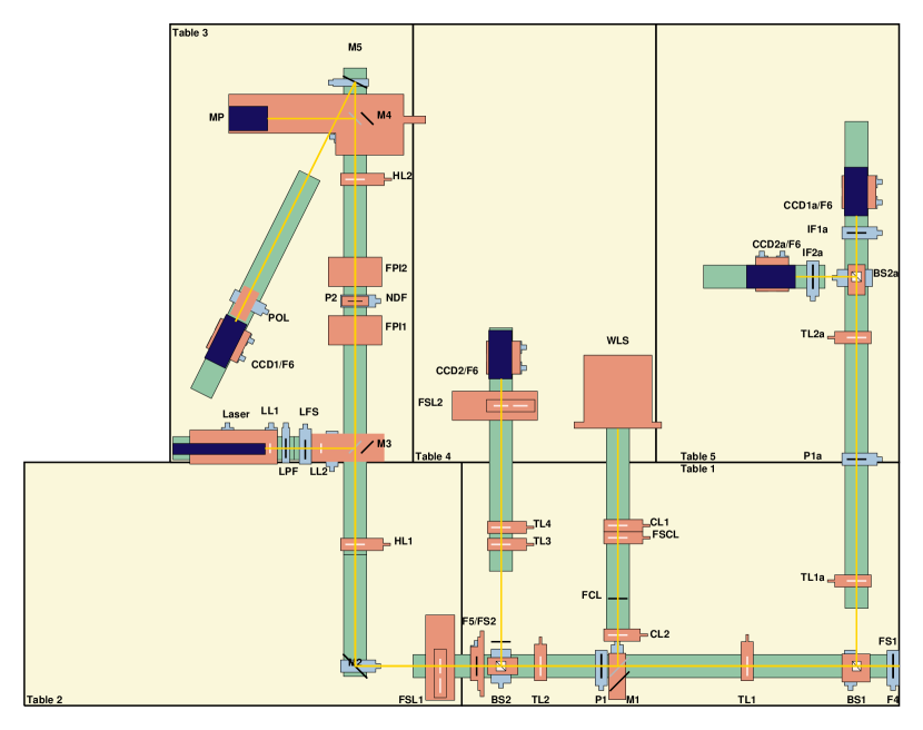
Figure 1: GFPI and blue imaging channel. CCD1 & CCD2: Imager QE detectors; CCD1a & CCD2a: pco.4000 detectors; FPI1 & FPI2: narrow-band etalons; NDF: neutral density filter; TL1 ($f=600$ mm, $d=63$ mm), TL2 ($f=250$ mm, $d=40$ mm), TL1a ($f=500$ mm, $d=63$ mm), TL2a ($f=500$ mm, $d=80$ mm), TL3 ($f=400$ mm, $d=63$ mm), TL4 ($f=600$ mm, $d=63$ mm), HL1 ($f=1000$ mm, $d=80$ mm), & HL2 ($f=1500$ mm, $d=100$ mm): achromatic lenses; CL1 ($f=300$ mm, $d=63$ mm) & CL2 ($f=150$ mm, $d=40$ mm): plano-convex lenses; M1, M3, & M4: removable folding mirrors; M2 & M5: fixed folding mirrors (60 mm $\times$ 85 mm); F4, F5, F6, & FCL: foci; P1, P1a, & P2: pupil images; BS1, BS2 & BS2a: beamsplitters (40 mm $\times$ 40 mm); FS1, FS2 & FSCL: field stops; WLS: white-light source (slide projector); FSL1 & FSL2: filter sliders; IF1a & IF2a: interference filters; POL: full-Stokes polarimeter; LL1 & LL2: laser lenses; LPF: laser polarization filter; LFS: laser field stop; and MP: photomultiplier.

3 GREGOR Fabry-Perot Interferometer

3.1 Optical design

The GFPI is mounted on five optical tables and is protected by an aluminum housing to prevent the pollution of the optics by dust and to reduce stray-light. The optical layout of the instrument is shown in Fig. 1. Behind the science focus F4, four achromatic lenses TL1, TL2, HL1, & HL2 create two more foci F5 & F6 and two pupil images P1 & P2 in the narrow-band channel NBC. The etalons FPI1 & FPI2 are placed in the vicinity of the secondary pupil in the collimated light beam. A neutral density filter NDF between the two etalons with a transmission of 63% reduces the inter-etalon reflexes. The beam in the NBC is folded twice by M2 & M5 at a distance of 500 mm and 400 mm from F5 and HL2, respectively, to minimize the instrument envelope. Two field stops FS1 & FS2 reduce stray-light, where the secondary field stop especially avoids an overlap of the two images created by the removable dual-beam full-Stokes polarimeter. A beamsplitter cube BS2 near F5 directs 5% of the light to the broad-band channel BBC. There, the two achromatic lenses TL3 & TL4 are chosen such that the image scale of the detectors CCD1 & CCD2 is exactly the same. A dichroic beamsplitter cube BS1 just behind the science focus F4 sends the blue part of the spectrum (below 530 nm) to the imaging channel. One-to-one imaging with the lenses TL1a & TL2a provides the option of recording broad-band images in parallel to GFPI and GRIS observations with two pco.4000 cameras CCD1a & CCD2a behind beamsplitter BS2a. This imaging channel will be replaced by the Blue Imaging Solar Spectrometer (BLISS) in the future.

Three computer-controlled precision translation stages facilitate automated observing sequences. The two stages FSL1 & FSL2 are used to switch between two sets of interference filters. The filters restrict the bandpass for BBC and NBC to a full-width at half-maximum (FWHM) of 10 nm and 0.3–0.8 nm, respectively. The pre-filters of each channel can be tilted to optimize the wavelength of the transmission maximum. A third stage inserts a deflection mirror M1 into the light path to take calibration data with a continuum light source for spectral calibration purposes. A laser/photo-multiplier channel for finesse adjustment of the etalons completes the optical setup.

3.2 Cameras, etalons, and control software

The GFPI data acquisition system consists of two Imager QE CCD cameras with Sony ICX285AL detectors, which have a full-well capacity of 18,000 e^- and a read-out noise of 4.5 e^-. The detectors have a spectral response from 320–900 nm with a maximum quantum efficiency of $\sim$60% at 550 nm. The chips have $1376\times 1040$ pixels with a size of 6.45 $\mu$m $\times$ 6.45 $\mu$m. The total chip size is 8.8 mm $\times$ 6.7 mm. The image scale at both cameras is 0.0361^′′ pixel^-1, which leads to a FOV of $49.7\mbox{${}^{\prime\prime}$}\times 37.6\mbox{${}^{\prime\prime}$}$ in the spectroscopic mode. The maximal blueshift due to the collimated mounting of the etalons is about 4.32 pm at 630 nm. The cameras are triggered by a programmable timing unit sending out analog TTL signals. The analog-digital conversion is carried out with 12-bit resolution. The data recorded by the cameras are passed via digital coaxial cables to the GFPI control computer and are stored on a RAID 0 system.

Two pco.4000 cameras in stock at the observatory can be used for imaging in the blue channel of the FPI. The pco.4000 camera has a full-well capacity of 60,000 e^- and a read-out noise of 11 e^-. The detector has a spectral response from 320–900 nm with a quantum efficiency of $\sim$32% ($\sim$45%) at 380 (530) nm. The pixel size is 9 $\mu$m $\times$ 9 $\mu$m, i.e., $4008\times 2672$ pixels yield a total chip size of 36 mm $\times$ 24 mm. The image scale at both cameras is 0.0315^′′ pixel^-1. To avoid vignetting of the beam by BS1 and BS2a only $2800\times 2200$ pixels can be used resulting in a FOV of $88.2\mbox{${}^{\prime\prime}$}\times 69.3\mbox{${}^{\prime\prime}$}$. Three interference filters for Ca ii H $\lambda 396.8$ nm, Fraunhofer G-band $\lambda 430.7$ nm, and blue continuum $\lambda 450.6$ nm with a $\mathrm{FWHM}=1$ nm and a transmission better than 60% are available for observations.

The two GFPI etalons manufactured by IC Optical Systems (ICOS) have a diameter of $\oslash=70$ mm, a measured finesse ${\cal F}\sim 46$, spacings $d=1.1$ and 1.4 mm, and a high-reflectivity coating ($R\sim 95$%) in the wavelength range from 530–860 nm. The resulting narrow transmission of the instrument is on the order of $\mathrm{FWHM}=1.9$–5.6 pm and leads to a theoretical spectral resolution of ${\cal R}=250,000$. All etalons are operated by three-channel CS100 controllers manufactured by ICOS. The cavity spacings are digitally controlled by the GFPI control computer via RS-232 communication. A thermally insulated box protects the pupil and the etalons from stray-light and air flows inside the instrument.

The communication between internal (cameras, etalons, and filter and mirror sliders) and peripheral devices (telescope, AO system, AO filter wheel, GPU, GRIS, etc.) is controlled by the software package DaVis from LaVision in Göttingen, which has been adapted to the needs of the spectrometer.[17, 23] The modification of the software for TCP/IP communication with external devices using DCP allows an easy implementation of automated observing procedures. All observing modes such as etalon adjustment, line finding, flat-fielding, recording of dark, pinhole, and target images, continuum scans, and recording of scientific data are now automated.

3.3 Polarimetry at GREGOR

The science verification time in 2012 is mostly devoted to spectroscopy at GREGOR. Polarimetric observations will follow in 2013. Nevertheless, a polarization model for the GREGOR telescope has already been developed,[21] which is time-dependent because of the alt-azimuthal mount of the telescope. The GPU[27] was developed by and built at AIP and can be inserted at the secondary focus of the telescope to determine the instrumental polarization, which is important for the calibration of polarimetric measurements. Since 2008, The GFPI is equipped with a full-Stokes polarimeter[19] that can be inserted in front of the detector in the NBC. The polarimeter consists of two ferro-electric liquid crystal retarders (FLCRs) and a modified Savart-plate. The first liquid crystal acts as a half-wave plate and the second one as a quarter-wave plate at a wavelength of 630 nm. The modified Savart-plate consists of two polarizing beamsplitters and an additional half-wave plate, which exchanges the ordinary and the extraordinary beam. With this configuration, the separation of the two beams is optimized and the orientation of the astigmatism in both beams is the same so that it can be corrected by a cylindrical lens. The present set of FLCRs yields a good efficiency in the spectral range from 580–660 nm. The integration of an automated calibration procedure for the GFPI will be an important milestone before starting polarimetric observations.

4 GFPI science verification

For a first characterization of the GFPI performance, we took several data sets in a technical campaign from 15 May to 1 June 2012. The AO system was not available because of technical problems with the control computer. Thus, our efforts have been restricted to an optimization of the system and to observations of test data for an estimate of intensity levels, image quality, spectral resolution, stray-light, and other performance indicators of the GFPI and its extended blue imaging channel. Several problems related to the RS-232 communication with the FPI controllers were resolved so that a stable finesse is now achieved for several days. In addition, the timing between cameras and etalons has been optimized to ensure that images are only taken when the etalon spacing has settled to its nominal value.

4.1 Imaging spectrometric data

Table 1: Summary of the GFPI observations.

Channel	$\lambda_{0}$ [nm]	$\Delta t$ [ms]	$I$ [counts]	PHA (F4)	PH (F3)	PH (F2)	TG	QS	SP	PF
NBC ($1\times 1$ binning)	543.3	40	02400	x	x	–	x	x	x	x
BBC ($1\times 1$ binning)	543.3	40	–	x	x	–	x	x	x	–
NBC ($2\times 2$ binning)	543.3	30	03500	–	–	–	x	x	–	x
NBC ($2\times 2$ binning)	557.6	40	02100	–	x	–	x	x	–	x
NBC ($2\times 2$ binning)	617.3	10	03200	–	x	–	x	x	–	x
Ca ii H	396.8	15	09230	x	x	x	x	x	x	–
G-band	430.7	06	10350	x	x	x	x	x	x	–
Blue continuum	450.6	03	11300	x	x	x	x	x	x	–

Note. — Central wavelength $\lambda_{0}$, exposure time $\Delta t$, and mean intensity $I$ for all observations (PHA: pinhole array, PH: pinhole, TG: target, QS: quiet Sun, SP: sunspot, and PF: pre-filter).

Table 2: NBC pre-filter characteristics.

Filter	$\lambda_{0}$ [nm]	FWHM [nm]	$T$ [%]	Binning	$\Delta T$ [ms]	$I$ [counts]	Frame rate [Hz]
ANDV11436	543.4	0.4	38	$1\times 1$	60   (100)	1200   (2000)	07   (5)
	543.4	0.4	38	$2\times 2$	30   (0)00	3500   (0)000	11   (0)
1100 BARR9	543.4	0.6	70	$1\times 1$	40   0(60)	1700   (2700)	07   (6)
ANDV5288	557.6	0.3	40	$2\times 2$	40   (0)00	2100   (0)000	11   (0)
DV5289 AM-32389	569.1	0.3	45	$1\times 1$	60   (100)	1200   (2000)	06   (5)
ANDV9330	617.3	0.7	80	$1\times 1$	20   0(60)	1200   (3400)	09   (6)
	617.3	0.7	80	$2\times 2$	10   (0)00	3200   (0)000	16   (0)

Note. — Continuum intensities $I$ at wavelengths $\lambda_{0}$ for filters with peak transmissions $T$ and exposure times $\Delta T$.

Three complete data sets with $2\times 2$ binning ($\sim$0.0722^′′ pixel^-1) were taken on 31 May and 1 June, which included images of the target TG and pinhole PH mounted in the AO filter wheel at F3 (telescope focal plane). The observations covered the spectral lines at 543.4 nm, 557.6 nm, and 617.3 nm. The Fe i $\lambda 543.4$ nm line had already been scanned on 27 May at full spatial resolution (0.0361^′′ pixel^-1) including images of a pinhole array in F4 (science focus at the entrance of the GFPI). Simultaneous BBC images were recorded (Tab. 1). Line scans with the GFPI were usually carried out using a step width of eight digital-analog (DA) steps, whereas the pre-filter scans were performed with one DA step. One DA step corresponds to 0.26–0.41 pm in the spectral range from 530–860 nm.

Broad-band data were taken in the blue imaging channel on 26 and 27 May 2012 just before the GFPI measurements. The observing scheme was the same for all available pre-filters, i.e., 396.8 nm, 430.7 nm, and 450.6 nm. In addition to a few observations of the quiet Sun and a sunspot, images of the target and pinhole in F3, the pinhole-array in F4, and the pinhole mounted in the GPU at F2 are also included. All data in the blue channel were taken with a combination of two spare lenses with $f=500$ mm and 1250 mm because a second lens with $f=500$ mm was not available, yet. Thus, the image scale of 0.0124^′′ pixel^-1 oversamples the diffraction limit at these wavelengths by a factor of about three. The proper image scale of 0.0315^′′ pixel^-1 will be obtained by one-to-one imaging.

4.2 Intensity estimates for the narrow-band channel

The wavelength $\lambda_{0}$, FWHM, and transmission $T$ of different NBC filters are summarized in Tab. 2 together with the selected binning, the counts at continuum wavelengths, and frame rates at a given exposure time $\Delta T$. The results reveal that at full spatial resolution very long exposure times of up to 100 ms are necessary to achieve at least 2000 counts in the continuum of most of the measured spectral lines for most of the filters with $T\sim 40$% and a $\mathrm{FWHM}\sim 0.3$–0.4 nm. As a consequence, one can reach only very low frame rates. A $2\times 2$-pixel binning speeds up the observations and reduces the exposure times. The situation changes when choosing filters with higher transmission. The 617.3 nm filter with $T\sim 80$% and a $\mathrm{FWHM}\sim 0.74$ nm yields reasonable frame rates and exposure times even without binning.

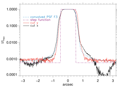
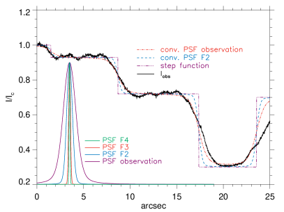
Figure 2: Derivation of the PSF estimate at 430 nm for the pinhole in F3 (left) and for the complete optical train from a sunspot observation (right), where the PSF estimates of the four different focal planes are displayed in the lower left corner.

4.3 Estimates of the spatial point spread function

Knowledge of the instrumental point spread function (PSF) provides an estimate of both the spatial resolution and the spatial stray-light level expected for an instrument or telescope.[30, 31] Using a reference such as a pinhole or a blocking edge in the focal plane, the PSF of all optics downstream can be derived. The combined PSF of the telescope, the post-focus instruments, and the time-variable seeing can also be derived from the observations of a sunspot with its steep spatial intensity gradients.

The PSF of the optical train at the GREGOR telescope relevant for the GFPI and its complementary imaging channels was calculated based on reduced images of pinholes located in the focal planes F4, F3, F2, and on sunspot images (see Tab. 1). All available calibration images, e.g., target or pinhole images, were averaged for each wavelength step or image burst. However, only a single image was selected for solar observations because the seeing varies during the image sequences. The pinhole images were normalized to the maximum intensity $I_{\rm max}$ inside the FOV near the center of the pinhole, whereas the sunspot data were normalized to unity in a quiet Sun region outside the spot. All data were taken without real-time correction of the AO system and consequently correspond to the static performance of the optical system.

4.4 Derivation of the point spread function estimates

We took cuts along the $x$- and $y$-axes of the CCD across the center of the pinhole in each pinhole observation to obtain an estimate of the PSF. We defined a step function that is assumed to represent the physical extent of the true pinhole. The borders of the step function were set to intersect the observed intensity along the cuts at about the 50% level (left panel of Fig. 2). We constructed a convolution kernel from a combination of a Gaussian (variance $\sigma$) and a Lorentzian function (parameter $a$) and convolved the step function with the kernel. A modification of the parameters ($\sigma,a$) within a specific range yielded finally the kernel that best matched the convolved step function and the observed intensity along the horizontal and vertical cuts. The cuts in $x$ and $y$ differed far away from the pinhole because of the read-out direction of the CCD camera. Thus, we always tried to find a good match to both the $x$- and $y$-cuts close to the pinhole. However, we concentrated only on matching the cut perpendicular to the CCD read-out direction away from the pinhole. The same method was applied to all pinhole observations (F4, F3, and F2) to derive a PSF estimate for each focal plane and wavelength. The sunspot observations were modeled by a similar step function at the two transitions from quiet Sun to penumbra and penumbra to umbra (right panel of Fig. 2).

The resulting PSF estimates of the four focal planes for the imaging data at 430.7 nm are displayed in the lower left corner of the right-hand panel of Fig. 2. The width of the PSF estimates is similar for F4 and F3, where only static optical components and negligible seeing effects contribute to the PSF and a diffraction-limited performance can be reached, but increases significantly when passing to the focal plane F2 that experiences telescope seeing and seeing fluctuations along the coudé train. The PSF derived from the sunspot observations includes all seeing effects and roughly doubles its width relative to the PSF at F2.

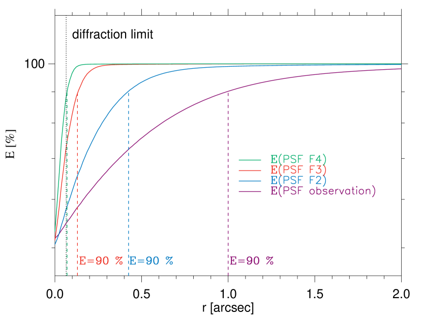
Channel	Imaging $\lambda 430.7$ nm				BBC $\lambda 543.4$ nm
Sampling	0.0124′′ pixel-1				0.034′′ pixel-1
	(0.0126′′ pixel-1)				(0.036′′ pixel-1)
Diff. limit	0.072′′				0.091′′
Focal plane	F4	F3	F2	Solar obs.	F4	F3	Solar obs.
$r$ ($E=90\%$)	0.07′′	0.13′′	0.43′′	1.00′′	0.11′′	0.17′′	2.4′′
$E$ ($r_{\mathrm{DL}}$)	90%	73%	58%	55%	85%	74%	52%

Channel	NBC $\lambda 543.4$ nm			NBC $\lambda 557.6$ nm	NBC $\lambda 617.3$ nm
Sampling	0.034′′ pixel-1			0.069′′ pixel-1	0.067′′ pixel-1
	(0.036′′ pixel-1)			(0.072′′ pixel-1)	(0.072′′ pixel-1)
Diff. limit	0.091′′			0.094′′	0.103′′
Focal plane	F4	F3	Solar obs.	F3	F3
$r(E=90\%)$	0.12′′	0.20′′	2.65′′	0.19′′	0.19′′
$E(r_{\mathrm{DL}})$	85%	71%	51%	75%	76%

Figure 3: Energy enclosed within the radius $r$ for the PSF estimates at 430.7 nm of the four different focal planes (left). The dashed vertical lines denote the radius where 90% of the energy is enclosed. The dotted vertical line denotes the diffraction limit at 430.7 nm. Similar observations were carried out at different wavelength (right). Theoretical values are given in parentheses.

By applying the approach described above to all available data, PSF estimates for all four focal planes were obtained in case of the imaging data at 430.7 nm, and for some of the focal planes in case of the GFPI BBC and NBC data (see table in Fig. 3). The optical performance and the expected stray-light level can best be quantified from the total energy enclosed in a given radius, i.e., a radial integration of the PSF whose volume yields the amount of light spread up to a given radius. Figure 3 shows the enclosed energy $E$ for the PSF estimates at 430.7 nm. From the curves, we derived two values, namely, the energy enclosed at the radius $E(r_{\mathrm{DL}})$ of the diffraction limit and the radius $r(E=90\%)$ at which 90% of the energy is enclosed. The former value provides an estimate of the generic stray-light to be expected by subtracting it from 100%. The latter value can be used as generic estimate of the spatial resolution. The table in Fig. 3 lists the two values for all analyzed wavelengths and channels, i.e., the blue imaging channel, and the GFPI BBC and NBC at specific wavelengths.

A comparison between the value of the diffraction limit and the radius where 90% of the energy is enclosed shows that the optics behind F4 performs close to diffraction limit. The optics downstream of F3 performs slightly worse with a total enclosed energy of about 70–75% of the diffraction-limited case. This implies a generic spatial stray-light level – if one defines stray-light as all light scattered to outside a distance of one times the diffraction limit – of about 25% created by the optics downstream of F3. The corresponding value at F4 is about 10–15%. The values of both the stray-light level and the radius that encloses 90% of the total energy experience a profound jump when passing to F2 and beyond. All these data were taken at mediocre seeing conditions and without AO correction. The latter will be necessary for a final characterization of the optical performance of the complete optical train including the telescope.

4.5 Spectral resolution, spectral stray-light, and blue-shift

The spectral resolution and the spectral stray-light inside the NBC was estimated by a convolution of Fourier Transform Spectrograph (FTS) atlas spectra with a Gaussian of width $\sigma$ and a subsequent addition of a constant wavelength-independent stray-light offset $\beta$.[32, 33] This component of stray-light corresponds to light scattered onto the CCD detector without being spectrally resolved. Therefore, it changes the line depth of observed spectral lines. The convolved FTS spectra in each wavelength range were compared with two sets of spatially averaged observational profiles that either covered the full pre-filter transmission curve or only the line inside the same range that is usually recorded in science observations (543.4 nm, 557.6 nm, 617.3 nm). The left panel of Fig. 4 shows the average observed spectrum at Fe i $\lambda 617.33$ nm, the original FTS spectrum, and the FTS spectrum after the convolution with the best-fit Gaussian kernel and the addition of the stray-light offset. The method has some ambiguity between $\sigma$ and $\beta$, which can be modified in opposite directions over some range near the best-fit values without significantly degrading the reproduction of the observed spectra. Therefore, the values listed in Tab. 3 have an error of about $\pm 0.5$ pm in $\sigma$ and $\pm 5$% in $\beta$. The stray-light level $\beta$ inside the GFPI is found to be below 10% and the spectral resolution is ${\cal R}\sim 100,000$, quite below the theoretically expected value of ${\cal R}\sim 250,000$. The dispersion values derived from the observed spectra are listed in Tab. 3 and correspond to eight DA steps. They match the theoretically expected values given in parentheses.

Table 3: Spectral characteristics of the GFPI data.

$\lambda$	Dispersion (8 DA)	Dispersion (1 DA)	$\sigma$	$\beta$	$\lambda/\sigma$	$\lambda/\Delta\lambda$	Max. blue-shift
[nm]	[pm]	[pm]	[pm]	[%]	–	–	[pm]
543.4	2.0800(2.09)	(0.261)	2.62	6.6	207189	088166	3.9100(3.72)
557.6	2.1500(2.15)	(0.268)	2.07	6.5	269453	114661	3.9600(3.82)
617.3	2.3600(2.36)	(0.296)	2.81	7.8	219695	093487	4.4900(4.23)
00630.25[12]	2.3100(2.41)		1.65	14	381818	162476	000000(4.32)

Note. — Theoretical values are indicated in parentheses.

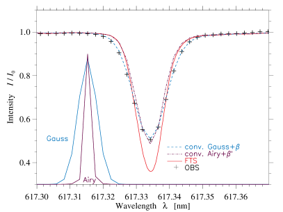
Figure 4: Close-up of the Fe i $\lambda 617.3$ nm spectral line at reduced spectral sampling (left): observed spectrum (black pluses), FTS atlas spectrum (red solid line), FTS convolved with the theoretical Airy function (orange dash-dotted line), and FTS convolved with the best-fit Gaussian kernel (blue dashed line). An appropriate stray-light offset ($\beta^{\prime},\beta$) was added after the convolution. The Airy function and the Gaussian kernel in the left corner are displayed in arbitrary units. Scan of the pre-filter curve around the $\lambda 543.4$ nm line at maximal spectral sampling (right).

For comparison, the FTS spectrum was convolved with the theoretical Airy function that describes the transmission through the double-etalon system using the measured finesse of 46. In this case, the line depth after the convolution could be adjusted by a stray-light offset $\beta^{\prime}$ of about 20%, but the observed line width in the wings of the line is not matched (Fig. 4). The performance of the GFPI in terms of the spectral resolution depends on the exact alignment of the plate parallelism of the etalons. For any detailed modeling of the spectral transmission it seems recommended to use a comparison of observed and atlas spectra instead of relying on the theoretically expected spectral PSF.

The measured finesse was obtained with a laser light source that produces a beam of about 15 mm diameter passing through the etalons. Therefore, the parallelism of the etalon plates was only optimized in the central part. In case of the observed spectra, the actual pupil diameter of P2 in the GFPI is about 60 mm and samples nearly the full surface of the etalons, in contrary to the VTT setup, where the pupil in the vicinity of the etalons still had a diameter of only about 40 mm. In the latter case, a spectral resolution still of ${\cal R}\sim 160,000$ was obtained applying the same method (see Tab. 3).

A degradation of the finesse between the central and peripheral regions of about 1.3 was found for a single etalon for radii of 15 mm and 50 mm.[34] The spectral resolution in the central area of the etalons of the GFPI at GREGOR would therefore be ${\cal R}\sim 170,000$, which is clearly above the thermal line width ($\lambda/\sigma_{th}\approx 134,000$). Note, however, that in this estimate similar effects of the second etalon are not yet considered. Thus, the effective spectral resolution of the central area might be even close to the value expected from theory. A widening of the laser beam, and consequently the adjustment of the finesse over a broader area fraction, might significantly improve the results.

The maximal blueshift induced in the spectra because of placing the FPIs inside a collimated beam was determined from a set of flat-field data. The numbers are close to the theoretically expected values (last column of Tab. 3).

Table 4: Selected spectral lines in the range 380–500 nm.

Ion	Wavelength $\lambda$	Excitation potential $\chi$	Landé-factor $g$	Equivalent width	Comment
Fe i	384.998 nm	01.01 eV	0.00	0060.8 pm	blends
CN-band	388.300 nm
He	388.865 nm	19.73 eV			only prominences
H$\zeta$	388.905 nm	10.20 eV		0234.6 pm	only prominences
Fe i	392.922 nm	03.25 eV	2.50	0003.7 pm	weak line
Ca ii K	393.368 nm	00.00 eV		2025.3 pm
Ca ii H	396.849 nm	00.00 eV		1546.7 pm
H$\epsilon$	397.008 nm	10.20 eV			line wing Ca ii H
Fe i	404.583 nm	01.48 eV		0117.5 pm	blends
Fe i	406.539 nm	03.43 eV	0.00	0006.4 pm
Mn i	407.028 nm	02.19 eV	3.33	0006.6 pm	high priority
Sr ii	407.772 nm	00.00 eV		0042.8 pm	resonance line
Fe i	408.088 nm	03.29 eV	3.00	0006.1 pm	high priority
H$\delta$	410.175 nm	10.20 eV		0313.3 pm
Fe ii	430.318 nm	02.70 eV	1.47	0010.3pm	in G-band
G-band	430.500 nm
H$\gamma$	434.048 nm	10.20 eV		0285.5 pm
Fe i	440.476 nm	01.56 eV		0089.8 pm	low priority
Ba ii	455.404 nm	00.00 eV		0015.9 pm	resonance line
Mg i	457.110 nm	00.00 eV		0009.2 pm	resonance line
Fe i	461.321 nm	03.29 eV	0.00	0006.6 pm	near $g_{\mathrm{eff}}=2.5$ line
Cr i	461.367 nm	00.96eV	2.50	0006.2 pm	near $g_{\mathrm{eff}}=0$ line
Ti i	464.519 nm	01.73 eV	2.50	0001.6 pm	enhanced in spots
Fe i	470.495 nm	03.69 eV	2.50	0005.8 pm	high priority
H$\beta$	486.134 nm	10.20 eV		0368.0 pm
Fe i	470.178 nm	03.93 eV	1.50	0004.4 pm	near $g_{\mathrm{eff}}=0$ line
Ni i	491.203 nm	03.77 eV	0.00	0004.7 pm

The scans of the pre-filter transmission curve at maximal spectral sampling showed another spectral feature in the GFPI data whose origin remains unclear up to now. A beat with stable period and varying amplitude is superimposed on the spectral lines (right panel of Fig. 4 for 543.4 nm). This beat is observed in all spectra, independent of wavelength and pre-filter, and has been present since the integration of the second narrow-band etalon in 2007. Owing to the aforementioned modifications, the beat is now absolutely stable with time in position and amplitude for each filter. Forward or backward scanning of the spectrum yields identical results. Thus, a removal of the beat is straightforward using the white-light source as a reference.

5 BLue Imaging Solar Spectrometer

The spatial resolution of a telescope scales inversely proportional with the observed wavelength. Therefore, observations at short wavelengths (below 530 nm) offer the opportunity to obtain data with higher spatial resolution. This advantage is partly diminished by the seeing degradations and the smaller number of photons at shorter wavelengths. There are relatively few ground-based instruments for spectral observations in the blue spectral region.[35, 36, 37, 38] All of these observations were carried out with slit-spectrographs that permit only limited improvements by post-factum restoration techniques.[30] A Fabry-Pérot-based imaging spectrometer provides data suitable for sophisticated post-factum image restoration techniques to yield high spatial and spectral resolution data. This is the motivation for BLISS, which will supplant the blue imaging channel of the GFPI in the near future.

5.1 Interesting spectral lines in the blue part of the visible spectrum

In the wavelength range covered by BLISS, there are several spectral lines and two molecular bands of high scientific interest (Tab. 4 and Fig. 5). All Balmer-lines except H$\alpha$ are at shorter wavelengths than 530 nm, and the H and K lines of ionized calcium are the strongest lines in the visible part of the solar spectrum probing the chromosphere. Several photospheric resonance lines such as Mg i $\lambda 457$ nm, Sr ii $\lambda 407$ nm, and Ba ii $\lambda 455$ nm are found in blue part of the visible spectrum. Here, one also finds several magnetically insensitive lines ($g_{\mathrm{eff}}=0$)[39] and on the other hand lines exhibiting a Zeeman-triplet with splitting factors of $g_{\mathrm{eff}}=2.5$ and higher.[40] A special case is the pair Fe i $\lambda 461.32$ nm ($g_{\mathrm{eff}}=0$) and Cr i $\lambda 461.37$ nm ($g_{\mathrm{eff}}=2.5$) that can be recorded at the same time. The molecular bands of CH $\lambda 430$ nm (G-band) and CN $\lambda 388$ nm are well suited to investigate very small hot features in the solar photosphere.

Figure 5: Selected spectral lines in the range 380–500 nm (see Tab. 4). The name and central wavelength of all spectral lines are given at the top of each panel. Major (minor) tick marks are separated by 0.1 nm (10 pm). Note that the spectral coverage of the panels changes from row to row, i.e., 0.1 nm, 0.2 nm, 1.0 nm, and 1.0 nm (from top to bottom).

5.2 Optical design

The geometrical design of BLISS is depicted in Fig. 6, which shows its integration into the GFPI by replacing the blue imaging channel. Most of the optical components and their labels are identical to those in Fig. 1 so that any information can be directly taken from there. The calculations for this initial optical design revealed that a pupil P2 of about 70 mm diameter will be sufficient for an acceptable maximal blue-shift over the entire wavelength range at a given image scale and FOV. Thus, the design of BLISS itself is almost identical to the design of the GFPI, apart from a re-design of the camera lenses HL2 and TL4 in the NBC and BBC to obtain an adequate image scale. The schematical optical designs of both instruments are compared in Fig. 7. The diameter of the light beam at the different foci, pupils, and on the relevant optical surfaces has been calculated by means of geometrical optics and confirmed by ZEMAX ray-tracing as for the GFPI.[18] The ZEMAX ray-tracing is presented in Fig. 8.

If one considers the actual values of the usable diameter of the main mirror and the focal length of the GREGOR telescope, the size of the pupil P2 inside the GFPI (59 mm) is smaller than the value assumed in the original calculation in 2007 (63 mm). However, a modification of the parabolic collimator and camera mirrors of the AO system will bring the pupil diameter again closer to the original value. Nevertheless, by changing the focal length of TL2, the reduction of the pupil diameter is currently compensated in the design of BLISS (see Fig. 7).

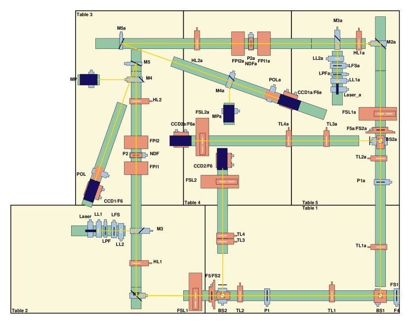
Figure 6: Geometrical design for the integration of BLISS into the GFPI system. The design is based on the study presented in Fig. 7. The optical elements of BLISS are labeled with an extra “a”. Apart from TL2a, HL2a, and TL4a, they are identical to those of the GFPI.

A new type of cameras has been envisaged for BLISS, namely, two sCMOS-cameras from PCO (pco.edge). These cameras have $2560\times 2160$ pixels with a pixel size of 6.5 $\mu$m $\times$ 6.5 $\mu$m similar to the GFPI Imager QE cameras. A change of the focal lengths of HL2 from $f=1500$ mm to $f=2250$ mm and of TL4 from $f=600$ mm to $f=900$ mm for BLISS (see Fig. 7) yields an image scale of 0.0276^′′ pixel^-1 and a FOV of $70.6\mbox{${}^{\prime\prime}$}\times 59.6\mbox{${}^{\prime\prime}$}$ on both cameras. With this configuration, the maximal blue-shift across the FOV amounts to 4.44 pm and 6.19 pm at 380 nm and 530 nm, respectively.

In addition, we checked the possibility of interchanging the sCMOS and Imager QE cameras between the GFPI and BLISS. The almost identical pixel sizes of both cameras facilitates this task. For the integration of the sCMOS cameras into the GFPI, a circular FOV with a diameter of $d=78.8\mbox{${}^{\prime\prime}$}$ and an image scale of 0.0364^′′ pixel^-1 for spectroscopy would result in a maximal blueshift of 6.91 pm at 630 nm. However, the FOV for polarimetry is limited by the full-Stokes polarimeter and would remain at its previous size of $24.9\mbox{${}^{\prime\prime}$}\times 37.6\mbox{${}^{\prime\prime}$}$. The frame rate at full resolution would increase from 7 to 40 Hz, which perfectly suits this observing mode.

The integration of the Imager QE cameras into BLISS would result in an image scale of 0.0274^′′ pixel^-1 and a FOV of $37.6\mbox{${}^{\prime\prime}$}\times 28.5\mbox{${}^{\prime\prime}$}$ with a maximum blueshift of 1.15 pm and 1.61 pm at 380 nm and 530 nm, respectively. The lower frame rates would match the longer exposure times at shorter wavelength. A super-achromatic optical setup for BLISS – as also foreseen for the GFPI – would be preferable but otherwise all lenses except TL4 of BLISS could be purchased as off-the-shelf achromats.

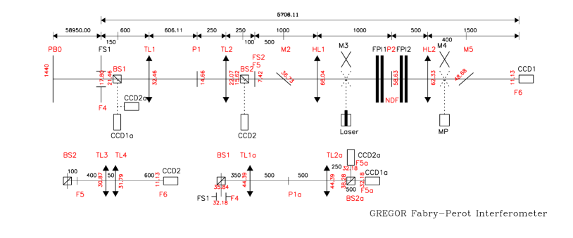
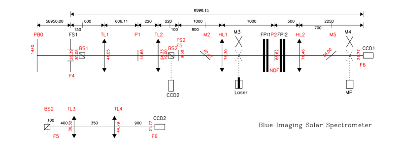
Figure 7: Schematical optical design (top) of the current GFPI NBC, BBC, and blue imaging channel. In the future, the BLISS NBC and BBC (bottom) will replace the GFPI blue imaging channel. The diameter of the beam at all optical surfaces, the focal length of the lenses, and the positions of other optical elements are given in millimeter. The achromatic lenses TL2, HL2, and TL4 of BLISS have a focal length of 220 mm, 2250 mm, and 900 mm, respectively. The mirrors M2 and M5 of the GFPI will be moved for the integration of BLISS by 200 mm and 50 mm, respectively.

The distribution of the two instruments on the five optical tables in the GREGOR observing room is shown in Fig. 6. All optical elements of BLISS have been labeled with an additional “a” to distinguish them from those of the GFPI. Behind the common dichroic beamsplitter cube BS1, each instrument has its own NBC and BBC. A displacement of the folding mirrors M2 and M5 of the GFPI to a distance of 700 mm and 350 mm from F5 and HL2, respectively, yields some free space on optical table 3 that can be used for the NBC of BLISS. The ZEMAX ray-tracing revealed changes in the optical path when considering the etalons plates in the design. Thus, the GFPI NBC has to be shortened further by reducing the distance between P2 and HL2 from 500 mm to 350 mm. This detail is not considered in Figs. 6 and 7.

The beam in the NBC of BLISS is also folded twice by M2a and M5a at a distance of 800 mm and 700 mm from F5a and HL2a, respectively. In the BBC of BLISS, TL3a and TL4a are separated by 350 mm, in contrary to the 50 mm between TL3 and TL4 in case of the GFPI. Two computer-controlled filter sliders FSL1a and FSL2a will again switch between two sets of interference filters, which restrict the bandpass for the BLISS BBC and NBC. BLISS is mainly designed for spectroscopy because of the expected low photon numbers in the blue spectral region. Nevertheless, a full-Stokes polarimeter can easily be integrated into the system. As in case of the GFPI, a laser/photo-multiplier channel for finesse adjustment of the etalons will be implemented. The white-light channel of the GFPI will be removed and be replaced by an external white-light source common to all instruments at GREGOR.

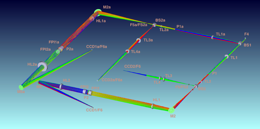
Figure 8: Total arrangement of GFPI and BLISS in a ZEMAX multi-configuration file in shaded modeling for the respective central wave length of each instrument and their maximal field dimension. The design confirms the calculations in geometrical optics presented in Figs. 6 and 7.

5.3 Camera system

Modern sCMOS cameras are capable of delivering high frame rates using large-format sensors with low readout noise, which makes them ideally suited for an application in solar physics. The pco.edge is a potential candidate for BLISS. The sensor of this camera has $2560\times 2160$ pixels with a size of 6.5 $\mu$m $\times$ 6.5 $\mu$m and a full well capacity of 30,000 e^-. The camera has a 16-bit digitization and would be operated in a global shutter mode. In this mode, the camera has a maximum frame rate of 40 Hz. The cameras are running in a “fast scan mode” (286 MHz) because of speed limitations of the camera link interface. The 16-bit signal is internally converted to 12-bit in the fast scan mode. Inside the interface it is decompressed again to 16-bit. The signal losses due to the compression are roughly a factor of ten smaller than the shot noise of the camera signal. The readout noise is in the order of 2.3 e^-. The dark current in the global shutter mode consists of a part related to the exposure time, i.e., 2–6 e^- pixel^-1 s^-1 and a part related to the sensor readout time, which is constant for a given pixel clock, i.e., 0.6 e^- pixel^-1 in the fast scan mode. Peltier cooling of the sensor ensures an operating temperature of $+5^{\circ}$ C. The camera has a quantum efficiency of $\sim$30% and $\sim$54% at 380 nm and 530 nm, respectively, similar to the Imager QE cameras currently used in the GFPI ($\sim$36% and $\sim$60%).

To handle the extremely large data bandwidth of about 300 MB s^-1 at frame rates of 40 Hz, each camera will be controlled by an individual PC, in which the data will be stored on local RAID 0 systems. The integration of the cameras in the control software is straightforward because the DaVis software will be operational on the new system with minor changes only. The cameras are currently being tested at AIP including, e.g., an analysis of image quality, power spectra, and noise characteristics.

However, the feasibility of using the pco.edge for BLISS has still to be demonstrated. A detailed photon statistic in the wavelength range 380–530 nm will help with the final decision, if these cameras will be employed in BLISS or the GFPI. For the blue wavelength range, rather long exposure times can be expected, making the use of high-speed cameras somewhat doubtful. Moreover, the exposure time of the cameras currently has an upper limit of 100 ms due to a relatively high dark current in the global shutter mode. On the other hand, high frame rates would be extremely beneficial when operating the GFPI in the vector polarimetric mode, because at present this instrument is limited to just 5–7 Hz at full resolution. The disadvantage would be just a partial usage of the chip. The almost identical pixel size facilitates interchanging the cameras between the two instruments.

Figure 9: Comparison of the GFPI (left)/BLISS (right) transmission profiles. The curves correspond to a narrow-band interference filter ($\mathrm{FWHM}=0.3$ nm, thin solid line), etalon 1 ($R=0.95/0.92$, $d=1.4/0.41$ mm, $\mathrm{FWHM}=2.1/5.2$ pm, thin dashed line), etalon 2 ($R=0.95/0.92$, $d=1.1/0.24$ mm, $\mathrm{FWHM}=2.7/8.9$ pm, thin dash-dotted line), and all transmission curves combined ($\mathrm{FWHM}=1.5/4.2$ pm, parasitic-light fraction 0.8/0.4%, thick solid line). The transmission profiles are normalized to unity at the central wavelength $\lambda_{0}=600.0/400.0$ nm.

5.4 Etalons

Airy functions are quasi-periodic, i.e., in a dual etalon system their characteristics parameters (reflectivity $R$ and plate separation $d$) have to be carefully chosen to minimize parasitic light from neighboring orders. Even if an optimal choice has been identified, narrow-band interference filters (0.3–0.8 nm) have to be used to minimize the contributions by the parasitic light. In general, an optimization of the characteristic FPI parameters has to include realistic transmission curves for the interference filters. In Fig. 9, we present the results of such a parameter study for BLISS and compare them with the case of the GFPI. The characteristic parameters of the BLISS etalons were chosen such that the parasitic light is minimized. The reflectivity of etalons for imaging in the blue spectral region has to be lower to increase the FWHM and to accommodate the smaller number of available photons. Therefore, the rejection of parasitic light further away from the central wavelength $\lambda_{0}$ becomes more important and narrower interference filters are required. The combination of etalons with $d=0.41$ and 0.24 mm ($\mathrm{FWHM}=5.2$ and 8.9 pm), will further increase the light level and result in a theoretical spectral resolution of ${\cal R}\sim 100,000$.

6 Data pipeline for imaging spectropolarimetry

Analyzing data from imaging spectropolarimetry requires intimate knowledge about seeing, telescope, Fabry-Pérot etalons, detector systems, instrumental polarization, and image restoration techniques. This knowledge about the entire image formation process has to be encapsulated in a reliable and robust data pipeline, which provides the user with well calibrated, self-describing data suitable for further analysis using, for example, spectral line inversion techniques.

The GFPI builds upon a two-decade heritage of Fabry-Pérot interferometers operated at the VTT. During this period the data reduction code bifurcated significantly necessitating rewriting the code from scratch. The best features of the individual codes were kept and in addition, the most time-consuming algorithm were tuned for performance.

6.1 Data processing and image restoration

Imaging spectropolarimetry[23, 12] offers the possibility to improve the recorded data beyond AO real-time correction. Therefore, several state-of-the-art image restoration techniques will be part of the GFPI data pipeline. At present, two of the most successful solar image restoration tools are included, namely, the Göttingen speckle imaging and deconvolution code[41, 42, 43] and Multi-Frame Blind Deconvolution[44] (MFBD) as well as its extension to multiple objects[45] (MOMFBD). As a third option the Kiepenheuer-Institute Speckle Interferometry Package[46, 47] (KISIP) will be included in the near future.

The data pipeline was developed in particular for data of the GFPI and BLISS. However, its modular approach to image processing facilitates the integration of other imaging spectropolarimeters. The I/O interface can be easily adapted. Since image restoration is an integral part of the data pipeline, also images from high-cadence, large-format CCD or CMOS cameras can be easily reduced. The information about observatories, telescopes, instruments, and detectors is kept in configuration files, which can simply be modified for site-specific needs.

The data pipeline is based on the Interactive Data Language (IDL). We adhere to a slightly modified version of the IDL coding standard[48] to provide the same “touch-and-feel” for all programs. This is enforced by using the same variable names in all programs, where descriptive variable names are the guiding principle rather than short names without meaning. The IDL source code of the GFPI data pipeline is available to all GFPI users. However, the hardware requirements go beyond that provided by typical work stations. Nevertheless, scaled-down data processing is still possible on a desk-top computer.

6.2 Data formats and data conversion

GFPI data are written in a native DaVis format, which uses on-the-fly image compression to achieve high data rates while writing data to a RAID 0 harddisk array. Narrow- and broad-band images are saved together in one file for each simultaneous exposure. Imaging spectropolarimetric sequences are accompanied by “set” files, i.e., an ASCII file with all information describing the data and observing modes. These compressed data are archived at AIP, whereas the principle investigator (PI) of the observing run receives a copy of the data in the Flexible Images Transport System[49] (FITS) format using image extensions[50]. Data from the GFPI data acquisition computer can be transferred by FTP to servers for data storage and processing, which are located at the VTT. The transfer lasts about the same time as taking the data. The raw data are then converted to FITS. Both data types are stored finally to LTO-Ultrium tapes with a storage capacity of about 800 GB.

6.3 Quick-look data, on-line repositories, and automatic logbooks

The data conversion step also includes several other tasks: (1) Image statistics are computed and included in the headers of the image extensions. These values are used in an heuristic error analysis to identify potential problems in the data acquisition process early on. Together with quantities describing the GFPI performance, they are stored in a database to monitor the long-term stability of the instrument and the quality of its data products. (2) Quick-look data products can be computed in time spans that are comparable to the data acquisition. Some functionality is already provided by the DaVis software (visualization of spectral scans, contrast enhancement, or region-of-interest manipulations). However, line-of-sight velocity maps or vector magnetograms have to be computed off-line. Limiting the image restoration to just a simple destretching of narrow- and broad-band images and taking averages at successive wavelength positions already provides spatially resolved information about the physical properties of the observed solar features. (3) Quick-look data are offered in two formats, either as web pages or as logbooks in the Portable Document Format (PDF), which both document each day’s observing run. The web pages with quick-look data will become public immediately, whereas the raw and FITS data will be embargoed for a certain time (typically one year), if the data are taken in the PI-mode.

6.4 Observing modes

Data from imaging spectropolarimetry can be analyzed in many different ways, for example, different image restoration methods are available, noise in both narrow- and broad-band images can be treated differently, or different schemes for the polarimetric correction of the data can be applied. All parameters describing a particular data processing scheme are saved in “project” files, which also serve as templates for observing runs with similar characteristics. This ensures that data products from different observing runs are comparable and enables their use in databases, where a user expects to have data products of the same quality.

Post-focus instruments at ground-based solar observatories are often operated in PI-mode, where the PI of an observing run specifies the instrument setup and observing sequences. The data are considered property of the PI and often only a small fraction of data finds its way into scientific publications. Changing this type of approach requires a concerted effort, both on the instrument-builder side and on the part of the developers of data pipelines. The GFPI control software offers a user interface for all standard data acquisition modes (dark, flat-field, target, and pinhole frames as well as spectral line scans). Interaction with the telescope, its subsystems, and other peripheral devices is handled automatically for each task. The “set” files for each mode contain all necessary information for further processing the data. The intermediate step of converting the data to FITS format allows the users to use their own data processing routines in addition to the GFPI data pipeline. A detailed account of the data processing is beyond the scope of this conference proceedings and will be deferred to a data release paper in a peer-reviewed journal.

- [1] Scharmer, G. B., Bjelksjo, K., Korhonen, T. K., Lindberg, B., and Petterson, B., “The 1-meter Swedish solar telescope,” in [Innovative telescopes and instrumentation for solar astrophysics ], Keil, S. L. and Avakyan, S. V., eds., Proc. SPIE 4853, 341–350 (2003).
- [2] Kosugi, T., Matsuzaki, K., Sakao, T., Shimizu, T., Sone, Y., Tachikawa, S., et al., “The Hinode (Solar-B) mission: an overview,” Sol. Phys. 243, 3–17 (2007).
- [3] Solanki, S. K., Barthol, P., Danilovic, S., Feller, A., Gandorfer, A., Hirzberger, J., et al., “SUNRISE: instrument, mission, data, and first results,” ApJL 723, L127–L133 (2010).
- [4] Volkmer, R., von der Lühe, O., Kneer, F., Staude, J., Balthasar, H., Berkefeld, T., et al., “New high resolution solar telescope GREGOR,” in [Modern solar facilities – advanced solar science ], Kneer, F., Puschmann, K. G. & Wittmann, A. D., ed., 39 (2007).
- [5] Volkmer, R., von der Lühe, O., Denker, C., Solanki, S., Balthasar, H., Berkefeld, T., et al., “GREGOR telescope: start of commissioning,” in [Ground-based and airborne telescopes III ], Stepp, L. M., Gilmozzi, R., and Hall, H. J., eds., Proc. SPIE 7733, 77330K (2010).
- [6] Volkmer, R., von der Lühe, O., Denker, C., Solanki, S. K., Balthasar, H., Berkefeld, T., et al., “GREGOR solar telescope: design and status,” Astronomische Nachrichten 331, 624 (2010).
- [7] Schmidt, W., von der Lühe, O., Volkmer, R., Denker, C., Solanki, S., Balthasar, H., et al., “The GREGOR solar telescope on Tenerife,” ASP Conf. Ser., in press, ArXiv e-prints, 2012arXiv1202.4289S (2012).
- [8] Denker, C., Goode, P. R., Ren, D., Saadeghvaziri, M. A., Verdoni, A. P., Wang, H., et al., “Progress on the 1.6-meter New Solar Telescope at Big Bear Solar Observatory,” in [Ground-based and airborne telescopes ], Stepp, L. M., ed., Proc. SPIE 6267, 62670A (2006).
- [9] Cao, W., Gorceix, N., Coulter, R., Coulter, A., and Goode, P. R., “First light of the 1.6 meter off-axis New Solar Telescope at Big Bear Solar Observatory,” in [Ground-based and airborne telescopes III ], Proc. SPIE 7733, 773330-773330-8 (2010).
- [10] Wagner, J., Rimmele, T. R., Keil, S., Hubbard, R., Hansen, E., Phelps, L., et al., “Advanced Technology Solar Telescope: a progress report,” in [Ground-based and airborne telescopes II ], Stepp, L. M. and Gilmozzi, R., eds., Proc. SPIE 7012, 70120I (2008).
- [11] Collados, M., Bettonvil, F., Cavaller, L., Ermolli, I., Gelly, B., Grivel-Gelly, C., et al., “European Solar Telescope: project status,” in [Ground-based and airborne telescopes III ], Stepp, L. M., R., G., and Hall, H. J., eds., Proc. SPIE 7733, 77330H (2010).
- [12] Puschmann, K. G. and Beck, C., “Application of speckle and (multi-object) multi-frame blind deconvolution techniques on imaging and imaging spectropolarimetric data,” A&A 533, A21 (2011).
- [13] Martínez Pillet, V., Del Toro Iniesta, J. C., Álvarez-Herrero, A., Domingo, V., Bonet, J. A., González Fernández, L., et al., “The Imaging Magnetograph eXperiment (IMaX) for the Sunrise balloon-borne solar observatory,” Sol. Phys. 268, 57–102 (2011).
- [14] Rimmele, T. R., Wagner, J., Keil, S., Elmore, D., Hubbard, R., Hansen, E., et al., “The Advanced Technology Solar Telescope: beginning construction of the world’s largest solar telescope,” in [Ground-based and Aiborne Telescopes III ], Stepp, L. M. and Gilmozzi, R., and Helen, H., eds., Proc. SPIE 7733, 77330G-17 (2010).
- [15] Bendlin, C., Volkmer, R., and Kneer, F., “A new instrument for high resolution, two-dimensional solar spectroscopy,” A&A 257, 817–823 (1992).
- [16] Volkmer, R., Kneer, F., and Bendlin, C., “Short-period waves in small-scale magnetic flux tubes on the Sun.,” A&A 304, L1 (1995).
- [17] Puschmann, K. G., Kneer, F., Seelemann, T., and Wittmann, A. D., “The new Göttingen Fabry-Pérot spectrometer for two-dimensional observations of the Sun,” A&A 451, 1151–1158 (2006).
- [18] Puschmann, K. G., Kneer, F., Nicklas, H., and Wittmann, A. D., “From the ”Göttingen” Fabry-Pérot interferometer to the GREGOR FPI,” in [Modern solar facilities – advanced solar science ], Kneer, F., Puschmann, K. G., and Wittmann, A. D., eds., 45 (2007).
- [19] Bello González, N. and Kneer, F., “Narrow-band full Stokes polarimetry of small structures on the Sun with speckle methods,” A&A 480, 265–275 (2008).
- [20] Balthasar, H., Bello González, N., Collados, M., Denker, C., Hofmann, A., Kneer, F., and Puschmann, K. G., “A full-Stokes polarimeter for the GREGOR Fabry-Pérot interferometer,” in [Cosmic Magnetic Fields: From Planets, to Stars and Galaxies ], Strassmeier, K. G., Kosovichev, A. G., and Beckman, J. E., eds., IAU Symp. 259, 665–666 (2009).
- [21] Balthasar, H., Bello González, N., Collados, M., Denker, C., Feller, A., Hofmann, A., et al., “Polarimetry with GREGOR,” in [Solar polarization 6 ], Kuhn, J. R., Harrington, D. M., Lin, H., Berdyugina, S. V., Trujillo-Bueno, J., Keil, S. L., and Rimmele, T., eds., ASP Conf. Ser. 437, 351 (2011).
- [22] Denker, C., Balthasar, H., Hofmann, A., Bello González, N., and Volkmer, R., “The GREGOR Fabry-Pérot interferometer: a new instrument for high-resolution solar observations,” in [Ground-based and airborne instrumentation for astronomy III ], McLean, I. S., Ramsay, S. K., and Takami, H., eds., Proc. SPIE 7735, 77356M–77356M–12 (2010).
- [23] Puschmann, K. G., Balthasar, H., Bauer, S. M., Hahn, T., Popow, E., Seelemann, T., et al., “The GREGOR Fabry-Pérot Interferometer – a new instrument for high-resolution spectropolarimetric solar observations,” ASP Conf. Ser., in press, ArXiv e-prints, 2011arXiv1111.5509P (2011).
- [24] Strassmeier, K. G., Woche, M., Granzer, T., Andersen, M. I., Schmidt, W., and Koubsky, P., “Gregor@Night,” in [Modern solar facilities – advanced solar science ], Kneer, F., Puschmann, K. G. & Wittmann, A. D., ed., 51 (2007).
- [25] Bettonvil, F. C. M., Hammerschlag, R. H., Jägers, A. P. L., and Sliepen, G., “Large fully retractable telescope enclosures still closable in strong wind,” in [Advanced Optical and Mechanical Technologies in Telescopes and Instrumentation ], Proc. SPIE 7018, 70181N-70181N-9 (2008).
- [26] Berkefeld, T., Soltau, D., Schmidt, D., and von der Lühe, O., “Adaptive optics development at the German solar telescopes,” Appl. Optics 49, G155 (2010).
- [27] Hofmann, A., Rendtel, J., and Arlt, K., “Toward polarimetry with GREGOR – testing the GREGOR Polarimetric Unit,” Centr. Eur. Astrophys. Bull. 33, 317–325 (2009).
- [28] Collados, M., Calcines, A., Díaz, J. J., Hernández, E., López, R., and Páez, E., “A high-resolution spectrograph for the solar telescope GREGOR,” in [Ground-based and airborne instrumentation for astronomy II ], McLean, I. S. and Casali, M. M., eds., Proc. SPIE 7014, 70145Z (2008).
- [29] Beck, C., Mikurda, K., Bellot Rubio, L. R., Kentischer, T., and Collados, M., “Multi-wavelength observations at the German VTT on Tenerife,” in [Modern solar facilities - advanced solar science ], Kneer, F., Puschmann, K. G., and Wittmann, A. D., eds., 55 (2007).
- [30] Beck, C., Rezaei, R., and Fabbian, D., “Stray-light contamination and spatial deconvolution of slit-spectrograph observations,” A&A 535, A129 (2011).
- [31] Löfdahl, M. G. and Scharmer, G. B., “Sources of straylight in the post-focus imaging instrumentation of the Swedish 1-m Solar Telescope,” A&A 537, A80 (2012).
- [32] Allende Prieto, C., Asplund, M., and Fabiani Bendicho, P., “Center-to-limb variation of solar line profiles as a test of NLTE line formation calculations,” A&A 423, 1109–1117 (2004).
- [33] Cabrera Solana, D., Bellot Rubio, L. R., Beck, C., and Del Toro Iniesta, J. C., “Temporal evolution of the Evershed flow in sunspots. I. Observational characterization of Evershed clouds,” A&A 475, 1067–1079 (2007).
- [34] Denker, C. and Tritschler, A., “Measuring and Maintaining the Plate Parallelism of Fabry-Pérot Etalons,” PASP 117, 1435–1444 (2005).
- [35] Lites, B. W., Rutten, R. J., and Kalkofen, W., “Dynamics of the solar chromosphere. I - Long-period network oscillations,” ApJ 414, 345–356 (1993).
- [36] Rouppe van der Voort, L. H. M., “Penumbral structure and kinematics from high-spatial-resolution observations of Ca II K,” A&A 389, 1020–1038 (2002).
- [37] Beck, C., Schmidt, W., Kentischer, T., and Elmore, D., “Polarimetric Littrow Spectrograph - instrument calibration and first measurements,” A&A 437, 1159–1167 (2005).
- [38] Beck, C., Schmidt, W., Rezaei, R., and Rammacher, W., “The signature of chromospheric heating in Ca II H spectra,” A&A 479, 213–227 (2008).
- [39] Sistla, G. and Harvey, J. W., “Fraunhofer lines without Zeeman splitting,” Sol. Phys. 12, 66–68 (1970).
- [40] Harvey, J. W., “Fraunhofer lines with large Zeeman splitting,” Sol. Phys. 28, 9–13 (1973).
- [41] de Boer, C. R., Speckle-Interferometrie und ihre Anwendungen auf die Sonnenbeobachtung, PhD thesis, Universitäts-Sternwarte Göttingen, Germany (1993).
- [42] Puschmann, K. G. and Sailer, M., “Speckle reconstruction of photometric data observed with adaptive optics,” A&A 454, 1011–1019 (2006).
- [43] Denker, C., Deng, N., Rimmele, T. R., Tritschler, A., and Verdoni, A., “Field-dependent adaptive optics correction derived with the spectral ratio technique,” Sol. Phys. 241, 411–426 (2007).
- [44] Löfdahl, M. G., “Multi-frame blind deconvolution with linear equality constraints,” in [Image reconstruction from incomplete data II ], Bones, P. J., Fiddy, M. A., and Millane, R. P., eds., Proc. SPIE 4792, 146–155 (2002).
- [45] van Noort, M., Rouppe van der Voort, L., and Löfdahl, M. G., “Solar image restoration by use of multi-frame blind de-convolution with multiple objects and phase diversity,” Sol. Phys. 228, 191–215 (2005).
- [46] Wöger, F., von der Lühe, O., and Reardon, K., “Speckle interferometry with adaptive optics corrected solar data,” A&A 488, 375–381 (2008).
- [47] Wöger, F. and von der Lühe, O., “KISIP: a software package for speckle interferometry of adaptive optics corrected solar data,” in [Advanced software and control for astronomy II ], Bridger, A. and Radziwill, N. M., eds., Proc. SPIE 7019, 70191E (2008).
- [48] Excelis Visual Information Solutions, “One proposal for an IDL coding standard,” Article ID 4120 (2006).
- [49] Hanisch, R. J., Farris, A., Greisen, E. W., Pence, W. D., Schlesinger, B. M., Teuben, P. J., et al., “Definition of the Flexible Image Transport System (FITS),” A&A 376, 359–380 (2001).
- [50] Ponz, J. D., Thompson, R. W., and Munoz, J. R., “The FITS image extension,” A&ASS 105, 53–55 (1994).