Compressed Sensing of Approximately-Sparse Signals: Phase Transitions and Optimal Reconstruction

Abstract

Compressed sensing is designed to measure sparse signals directly in a compressed form. However, most signals of interest are only “approximately sparse”, i.e. even though the signal contains only a small fraction of relevant (large) components the other components are not strictly equal to zero, but are only close to zero. In this paper we model the approximately sparse signal with a Gaussian distribution of small components, and we study its compressed sensing with dense random matrices. We use replica calculations to determine the mean-squared error of the Bayes-optimal reconstruction for such signals, as a function of the variance of the small components, the density of large components and the measurement rate. We then use the G-AMP algorithm and we quantify the region of parameters for which this algorithm achieves optimality (for large systems). Finally, we show that in the region where the G-AMP for the homogeneous measurement matrices is not optimal, a special “seeding” design of a spatially-coupled measurement matrix allows to restore optimality.

I Introduction

Compressed sensing is designed to measure sparse signals directly in a compressed form. It does so by acquiring a small number of random linear projections of the signal and subsequently reconstructing the signal. The interest in compressed sensing was boosted by works [1, 2] that showed that this reconstruction is computationally feasible in many cases. Often in the studies of compressed sensing the authors require that the reconstruction method works with guarantees for an arbitrary signal. This requirement then has to be paid by higher measurement rates than would be necessary if the probabilistic properties of the signal were at least approximately known. In many situations where compressed sensing is of practical interest there is a good knowledge about the statistical properties of the signal. In the present paper we will treat this second case.

It has been shown recently [3, 4] that for compressed sensing of sparse signals with known empirical distribution of components the theoretically optimal reconstruction can be achieved with the combined use of G-AMP algorithm [5, 6] and seeding (spatially coupled) measurement matrices. Actually, [3] argued that for noiseless measurements the knowledge of the signal distribution is not even required. It is well known that for noiseless measurements exact reconstruction is possible down to measurement rates equal to the density of non-zero components in the signal. For noisy measurements the optimal achievable mean-squared error (MSE) has been analyzed and compared to the performance of G-AMP in [7].

In its most basic form compressed sensing is designed for sparse signals, but most signals of interest are only “approximately sparse”, i.e. even though the signal contains only a small fraction of relevant (large) components the other components are not strictly equal to zero, but are only close to zero. In this paper we model the approximately sparse signal by the two-Gaussian distribution as in [8]. We study the optimal achievable MSE in the reconstruction of such signals and compare it to the performance of G-AMP algorithm using its asymptotic analysis - the state evolution [5, 6, 7]. Even-though we limit ourselves to this special class of signals and assume their knowledge, many qualitative features of our results stay true for other signals and when the distribution of signal-components is not known as well.

I-A Definitions

We study compressed sensing for approximately sparse signals. The $N$-dimensional signals that we consider have iid components, $K$ of these components are chosen from a distribution $\phi(x)$, we define the density $\rho=K/N$, and the remaining $N-K$ components are Gaussian with zero mean and small variance $\epsilon$

$$P({\textbf{x}})=\prod_{i=1}^{N}[\rho\phi(x_{i})+(1-\rho){\cal N}(0,\epsilon)]$$ (1)

Of course no real signal of interest is iid, however, for the same reasons as in [4] our analysis applies also to non-iid signals with empirical distribution of components converging to $\rho\phi(x)+(1-\rho){\cal N}(0,\epsilon)$. For concreteness our numerical examples are for Gaussian $\phi(x)$ of zero mean and unit variance. Although the numerical results depend on the form of $\phi(x)$, the overall picture is robust with respect to this choice. We further assume that the parameters of $P({\textbf{x}})$ are known or can be learned via expectation-maximization-type of approach.

We obtain $M$ measurements $y_{\mu}$ as linear projections of a $N$-components signal

$$y_{\mu}=\sum_{i=1}^{N}F_{\mu i}s_{i}\,,\quad\quad\mu=1,\dots,M\,.$$ (2)

The $M\times N$ measurement matrix is denoted $F_{\mu i}$. For simplicity we assume the measurements to be noiseless, the case of noisy measurements can be treated in the same way as in [7]. As done traditionally, in the first part of this paper, we consider the measurement matrix having iid components of zero mean and variance $1/N$. In our numerical experiments we chose the components of the matrix to be normally distributed, but the asymptotic analysis does not depend on the details of the components distribution. The seeding measurement matrices considered in the second part of this paper will be defined in detail in section IV.

The goal of compressed sensing is to reconstruct the signal s based on the knowledge of $M$ measurements y and the $M\times N$ matrix F. We define $\alpha=M/N$ to be the measurement (sampling) rate. The Bayes optimal way of estimating a signal ${\textbf{x}}^{\star}$ that minimizes the MSE $E=\sum_{i=1}^{N}(s_{i}-x_{i}^{\star})^{2}/N$ with the true signal s is given as

$$x^{\star}_{i}=\int\text{d}x_{i}\,x_{i}\,\nu_{i}(x_{i})\,,$$ (3)

where $\nu_{i}(x_{i})$ is the marginal probability distribution of the variable $i$

$$\nu_{i}(x_{i})\equiv\int_{\{x_{j}\}_{j\neq i}}P({\textbf{x}}|{\textbf{y}})\prod_{j\neq i}dx_{j}$$ (4)

under the posterior measure

$$P({\textbf{x}}|{\textbf{y}})=\frac{1}{Z({\textbf{y}})}P({\textbf{x}})\prod_{\mu=1}^{M}\delta(y_{\mu}-\sum_{i=1}^{N}F_{\mu i}x_{i})\,.$$ (5)

In this paper we will use an asymptotic replica analysis of this optimal Bayes reconstruction, which allows to compute the MSE as function of the parameters of the signal distribution, $\rho$ and $\epsilon$, and of the measurement rate $\alpha$.

Of course optimal Bayes reconstruction is not computationally tractable. In order to get an estimate of the marginals $\nu_{i}(x_{i})$, we use the G-AMP algorithm that is a belief-propagation based algorithm.

I-B Related works

The $\ell_{1}$-minimization based algorithms [1, 2] are widely used for compressed sensing of approximately sparse signals. They are very general and provide good performances in many situations. They, however, do not achieve optimal reconstruction when the statistical properties of the signal are known.

The two-Gaussian model for approximately sparse signal eq. (1) was used in compressed sensing e.g. in [8, 9].

Belief propagation based reconstruction algorithms were introduced in compressed sensing by [8]. Authors of [8] used sparse measurement matrices and treated the BP messages as probabilities over real numbers, that were represented by a histogram. The messages, however, can be represented only by their mean and variance as done by [10, 11]. Moreover, one does not need to send messages between every signal-components and every measurements [12], this leads to the approximate message passing (AMP). In the context of physics of spin glasses this transformation of the belief propagation equations corresponds to the Thouless-Anderson-Palmer equations [13]. The AMP was generalized for general signal models in [5, 6] and called G-AMP. The algorithm used in [3, 7] is equivalent to G-AMP. We also want to note that we find the name “approximate” message passing a little misleading since, as argued e.g. in [7], for dense random measurement matrices the G-AMP is asymptotically equivalent to BP, i.e. all the leading terms in $N$ are included in G-AMP.

For random matrices the evolution of iterations of G-AMP on large system sizes is described by state evolution [12]. The exactness of this description was proven in large generality in [14]. See also [15, 6, 7] for discussions and results on the state evolution.

The optimal reconstruction was studied extensively in [16]. The replica method was used to analyse the optimal reconstruction in compressed sensing in e.g. [17, 18]. In the statistical physics point of view the replica method is closely related to the state evolution [7].

As we shall see the G-AMP algorithm for homogeneous measurement matrices matches asymptotically the performance of the optimal reconstruction in a large part of the parameter space. In some region of parameters, however, it is suboptimal. For the sparse signals, it was demonstrated heuristically in [3] that optimality can be restored using seeding matrices (the concept is called spatial coupling), rigorous proof of this was worked out in [4]. The robustness to measurement noise was also discussed in [4, 7]. Note that the concept of “spatial coupling” thanks to which theoretical thresholds can be saturated was developed in error-correcting codes [19, 20, 21]. In compressed sensing the “spatial coupling” was first tested in [9] who did not observe any improvement for the two-Gaussian model for reasons that we will clarify later in this paper. Basically, the spatial coupling provides improvements only if a first order phase transition is present, but for the variance of small components that was tested in [9] there is no such transition: it appears only for slightly smaller values of the variance.

I-C Our Contribution

Using the replica method, we study the MSE in optimal Bayes inference of approximately sparse signals. In parallel, we study the asymptotic (large $N$) performance of G-AMP using state evolution. The parameters that we vary are the density of large components $\rho=K/N$, the variance of the small components $\epsilon$ and the sampling rate $\alpha=M/N$.

More precisely, we show that for a fixed signal density $\rho$, for low variance of the small components $\epsilon<\epsilon(\rho)$, the optimal Bayes reconstruction has a transition at a critical value $\alpha=\alpha_{\rm opt}$, separating a phase with a small value (comparable to $\epsilon$) of the MSE, obtained at $\alpha>\alpha_{\rm opt}$, from a phase with a large value of the MSE, obtained at $\alpha<\alpha_{\rm opt}$. This is a “first order” phase transition, in the sense that the MSE is discontinuous at $\alpha=\alpha_{\rm opt}$.

The G-AMP algorithm exhibits a double phase transition. It is asymptotically equivalent to the optimal Bayes inference at large $\alpha_{\rm BP}<\alpha<1$, where it matches the optimal reconstruction with a small value of the MSE. At low values of $\alpha<\alpha_{\rm opt}$ the G-AMP is also asymptotically equivalent to the optimal Bayes inference but in this low-sampling-rate region the optimal result leads to a large MSE. In the intermediate region $\alpha_{\rm opt}<\alpha<\alpha_{\rm BP}$ G-AMP leads to large MSE, but the optimal Bayes inference leads to low MSE. This is the region where one needs to improve on G-AMP. We show that in this intermediate region the G-AMP performance can be improved with the use of seeding (spatially coupled) measurement matrices, and with a proper choice of the parameters of these matrices one can approach the performance of the optimal Bayes inference in the large system size limit.

Finally for higher variance of the small components $\epsilon>\epsilon(\rho)$ there is no phase transition for $0<\alpha<1$. In this regime, G-AMP achieves optimal Bayes inference and the MSE that it obtains varies continuously from 0 at $\alpha=1$ to large values at low measurement rate $\alpha$.

II Bayes optimal and G-AMP reconstruction of approximately sparse signals

If the only available information about the signal is the matrix F and the vector of measurements y then the information-theoretically best possible estimate of each signal component is computed as a weighted average over all solutions of the linear system (2), where the weight of each solution is given by (1). Of course, the undetermined linear system (2) has exponentially many (in $N$) solutions and hence computing exactly the above weighted average is in general intractable.

The corresponding expectation can be, however, approximated efficiently via the generalized approximate message passing (G-AMP) algorithm [6, 5, 3, 7] that we recall in Sec. II-A. The behavior of the algorithm in the limit of large system sizes can be analyzed via state evolution [14, 3, 7], as we recall in Sec. II-B.

The asymptotic performance of the optimal reconstruction can be analyzed via the replica method as in [17, 18, 7], which is closely related to the state evolution of the G-AMP algorithm. We summarize the corresponding equations in Sec. II-C.

II-A Reminder of the G-AMP Algorithm

The G-AMP is an iterative message passing algorithm. For every measurement component we define quantities $V_{\mu}$ and $\omega_{\mu}$, for each signal component quantities $\Sigma_{i}$, $R_{i}$, $a_{i}$, $v_{i}$. In the G-AMP algorithm these quantities are updated as follows (for the derivation in the present notation see [7], for the original derivation [6, 5])

$$V^{t+1}_{\mu} = \sum_{i}F_{\mu i}^{2}\,v^{t}_{i}\,,$$ (6)

$$\omega^{t+1}_{\mu} = \sum_{i}F_{\mu i}\,a^{t}_{i}-\frac{(y_{\mu}-\omega^{t}_{\mu})}{V^{t}_{\mu}}\sum_{i}F_{\mu i}^{2}\,v^{t}_{i}\,,$$ (7)

$$(\Sigma^{t+1}_{i})^{2} = \left[\sum_{\mu}\frac{F^{2}_{\mu i}}{V^{t+1}_{\mu}}\right]^{-1}\,,$$ (8)

$$R^{t+1}_{i} = a^{t}_{i}+\frac{\sum_{\mu}F_{\mu i}\frac{(y_{\mu}-\omega^{t+1}_{\mu})}{V^{t+1}_{\mu}}}{\sum_{\mu}\frac{F_{\mu i}^{2}}{V^{t+1}_{\mu}}}\,,$$ (9)

$$a^{t+1}_{i} = f_{a}\left((\Sigma^{t+1}_{i})^{2},R^{t+1}_{i}\right),$$ (10)

$$v^{t+1}_{i} = f_{c}\left((\Sigma^{t+1}_{i})^{2},R^{t+1}_{i}\right)\,.$$ (11)

Here only the functions $f_{a}$ and $f_{b}$ depend in an explicit way on the signal model $P({\textbf{x}})$. For the signal model (1) considered in this paper we have

$$f_{a}(\Sigma^{2},R)=\frac{\sum_{a=1}^{2}w_{a}e^{-\frac{R^{2}}{2(\Sigma^{2}+\sigma_{a}^{2})}}\frac{R\sigma_{a}^{2}}{(\Sigma^{2}+\sigma_{a}^{2})^{\frac{3}{2}}}}{\sum_{a=1}^{2}w_{a}\frac{1}{\sqrt{\Sigma^{2}+\sigma_{a}^{2}}}e^{-\frac{R^{2}}{2(\Sigma^{2}+\sigma_{a}^{2})}}}\,,$$ (12)

$$f_{b}(\Sigma^{2},R)=\frac{\sum_{a=1}^{2}w_{a}e^{-\frac{R^{2}}{2(\Sigma^{2}+\sigma_{a}^{2})}}\frac{\sigma_{a}^{2}\Sigma^{2}(\Sigma^{2}+\sigma_{a}^{2})+R^{2}\sigma_{a}^{4}}{(\Sigma^{2}+\sigma_{a}^{2})^{\frac{5}{2}}}}{\sum_{a=1}^{2}w_{a}\frac{1}{\sqrt{\Sigma^{2}+\sigma_{a}^{2}}}e^{-\frac{R^{2}}{2(\Sigma^{2}+\sigma_{a}^{2})}}}\,,$$

$$f_{c}(\Sigma^{2},R)=f_{b}(\Sigma^{2},R)-f_{a}^{2}(\Sigma^{2},R)\,.$$ (13)

For the approximately sparse signal that we consider in this paper we have

$$w_{1}=\rho\,,\quad\sigma_{1}^{2}=\sigma^{2}\,,$$ (14)

$$w_{2}=1-\rho\,,\quad\sigma_{2}^{2}=\epsilon\,.$$ (15)

A suitable initialization for the quantities is $a_{i}^{t=0}=0$, $v_{i}^{t=0}=(1-\rho)\epsilon+\rho\sigma^{2}$, $\omega_{\mu}^{t=0}=y_{\mu}$.

Once the convergence of the iterative equations is reached, i.e. the quantities do not change anymore under iterations, the estimate of the $i$th signal component is $a^{t}_{i}$. The MSE achieved by the algorithm is then $E^{t}=\sum_{i=1}^{N}(a_{i}^{t}-s_{i})^{2}/N$.

II-B Evolution of the algorithm

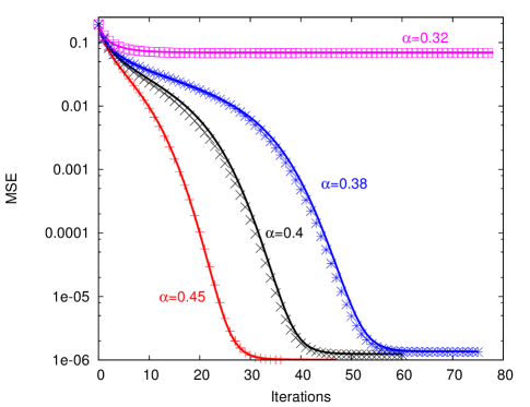
Figure 1: Time-evolution of the MSE the G-AMP algorithm achieves (points) compared to the asymptotic $N\to\infty$ evolution obtained from the state evolution eq. (16) (full lines). Data are obtained for a signal with density of large component $\rho=0.2$, variance of the small components $\epsilon=10^{-6}$. The algorithm was used for a signal of $N=3\cdot 10^{4}$ components.

In the limit of large system sizes, i.e. when parameters $\rho,\epsilon,\alpha$ are fixed whereas $N\to\infty$, the evolution of the G-AMP algorithm can be described exactly using the “state evolution” [14]. In the case where the signal model corresponds to the statistical properties of the actual signal, as it is the case in the present work, the state evolution is stated in terms of a single variable $E^{t}$, the MSE at iteration-time $t$, which evolves as (for a derivation see e.g. [14, 6, 7])

$$E^{t+1}=\sum_{a=1}^{2}w_{a}\int{\cal D}zf_{c}\left(\frac{1}{\hat{m}^{t}},z\sqrt{\sigma_{a}^{2}+\frac{1}{\hat{m}^{t}}}\right)\,,$$ (16)

$${\hat{m}}^{t}=\frac{\alpha}{E^{t}}\,,$$ (17)

where ${\cal D}z=e^{-z^{2}/2}/\sqrt{2\pi}dz$ is a Gaussian measure for the integral. The initialization corresponding to the one for the algorithm is $E^{t=0}=(1-\rho)\epsilon+\rho\sigma^{2}$.

In Fig. 1 we plot the analytical prediction for the time evolution of the MSE computed from the state evolution (16), and we compare it to the one measured in one run of the G-AMP algorithm for a system size $N=3\cdot 10^{4}$. The agreement for such system size is already excellent.

II-C Optimal reconstruction limit

We notice that for some measurement rates $\alpha$ the state evolution equation (16) has two different stable fixed points. In particular, if the iterations are initialized with $E\to 0$, for certain values of $\alpha$ one will reach a fixed point with much lower MSE than initializing with large $E$. In fact, one of the fixed points determines the MSE that would be achieved by the exact Bayes optimal inference. This can be seen using the heuristic replica method that leads to asymptotically exact evaluation of the logarithm of the partition function $Z$ in eq. (5). In general, if the partition function can be evaluated precisely then the expectations $x_{i}^{\star}$ eq. (3) and the associated MSE of the optimal inference can be computed.

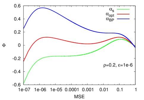
Figure 2: The potential function $\Phi(E)$ for signals of density $\rho=0.2$, with variance of the small components $\epsilon=10^{-6}$. The three lines depict the potential for three different measurement rates corresponding to the critical values: $\alpha_{\rm BP}=0.3559$, $\alpha_{\rm opt}=0.2817$, $\alpha_{s}=0.2305$. The two local maxima exists for $\alpha\in(\alpha_{s},\alpha_{\rm BP})$, at $\alpha_{\rm opt}$ the low MSE maxima becomes the global one.

The replica analysis, derived for the present problem e.g. in [7], shows that the large $N$ limit of $\log{Z}/N$ is equal to the global maximum of the following “potential” function

$$\Phi(E)= -\frac{\alpha}{2}\left(\log E+\frac{w_{1}\sigma_{1}^{2}+w_{2}\sigma_{2}^{2}}{E}\right)$$

$$+\sum_{a=1}^{2}w_{a}\int{\cal D}z\log{\left[\sum_{b=1}^{2}w_{b}\frac{e^{\frac{(\hat{m}^{2}\sigma_{a}^{2}+\hat{m})z^{2}}{2(\hat{m}+1/\sigma_{b}^{2})}}}{\sqrt{\hat{m}\sigma_{b}^{2}+1}}\right]}$$ (18)

Note that the state evolution corresponds to the steepest ascent of $\Phi(E)$. When $\Phi(E)$ has two local maxima then the fixed point of (16) depends on the initial condition.

In Fig. 2 we plot the function $\Phi(E)$ for a signal of density $\rho=0.2$, variance of small components $\epsilon=10^{-6}$ and three different values of the measurement rate $\alpha$. We define three phase transitions

• $\alpha_{\rm BP}$ is defined as the largest $\alpha$ for which the potential function $\Phi(E)$ has two local maxima.

• $\alpha_{s}$ is defined as the smallest $\alpha$ for which the potential function $\Phi(E)$ has two local maxima.

• $\alpha_{\rm opt}$ is defined as the value of $\alpha$ for which the two maxima have the same height.

III Phase diagrams for approximate sparsity

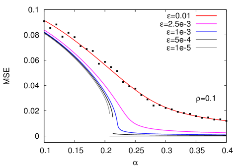
Figure 3: The MSE achieved by the G-AMP. The lines correspond to the evaluation of the MSE from the state evolution, the data points to the MSE achieved by the G-AMP algorithm for $N=3\cdot 10^{4}$. The data are for signals with density $\rho=0.1$ and several values of variance of small components $\epsilon$ as a function of the measurement rate $\alpha$. The MSE grows continuously as $\alpha$ decreases for $\epsilon>0.00075$. For smaller values of the noise a first order phase transition is present and the MSE jumps discontinuously at $\alpha_{\rm BP}(\epsilon)$.

In Fig. 3 we plot the MSE to which the state evolution converges if initialized at large value of MSE - such initialization corresponds to the iterations of G-AMP when the actual signal is not known. For $\epsilon=0.01$ we also compare explicitly to a run of G-AMP for system size of $N=3\cdot 10^{4}$. Depending on the value of density $\rho$, and variance $\epsilon$, two situations are possible: For relatively large $\epsilon$, as the measurement rate $\alpha$ decreases the final MSE grows continuously from $E=0$ at $\alpha=1$ to $E=E^{t=0}$ at $\alpha=0$. For lower values of $\epsilon$ the MSE achieved by G-AMP has a discontinuity at $\alpha_{\rm BP}$ at which the second maxima of $\Phi(E)$ appears. Note that the case of $\epsilon=0.01$ was tested in [8], the case of $\epsilon=0.0025$ in [9].

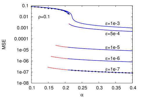
Figure 4: MSE achieved by the G-AMP (blue solid lines) compared to the MSE achieved by the Bayes-optimal inference (red dashed lines) as evaluated using the state evolution. The data points correspond to the MSE achieved by the G-AMP algorithm for $N=3\cdot 10^{4}$. The optimal MSE jumps at $\alpha_{\rm opt}$. Hence for $\epsilon<0.00075$ there is a range of measurement rates $(\alpha_{\rm opt,\alpha_{\rm BP}})$ in which the BP is asymptotically suboptimal.

In Fig. 4 we plot in full blue line the MSE to which the G-AMP converges and compare to the MSE achieved by the optimal Bayes inference, i.e. the MSE corresponding to the global maximum of $\Phi(E)$ (in dashed red line). We see that, when the discontinuous transition point $\alpha_{\rm BP}$ exists, then in the region $\alpha_{\rm opt}<\alpha<\alpha_{\rm BP}$ G-AMP is suboptimal. We remind that, in the limit$\epsilon\to 0$, exact reconstruction is possible for any $\alpha>\rho$. We see that for $\alpha<\alpha_{\rm opt}$ and for $\alpha>\alpha_{\rm BP}$ the performance of G-AMP matches asymptotically the performance of the optimal Bayes inference. The two regions are, however, quite different. For $\alpha<\alpha_{\rm opt}$ the final MSE is relatively large, whereas for $\alpha>\alpha_{\rm BP}$ the final MSE is of order $\epsilon$ and hence is this region the problem shows a very good stability towards approximate sparsity.

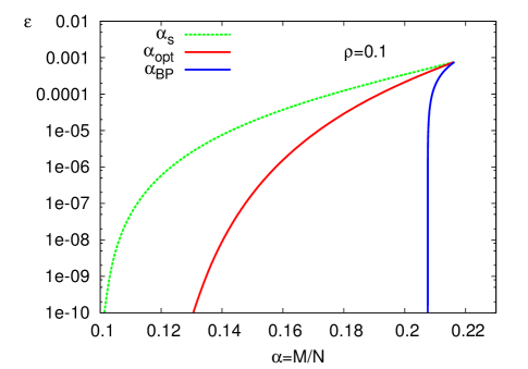
Figure 5: Phase diagram for compressed sensing of approximately sparse signals. The density of the large signal components is $\rho=0.1$, we are changing measurement rate $\alpha$ and variance of small components $\epsilon$. The critical values of measurement rates $\alpha_{\rm opt}$, $\alpha_{BP}$ and $\alpha_{s}$ are plotted. For homogeneous measurement matrices, BP does not achieve optimal reconstruction in the area between $\alpha_{\rm opt}$ (red) and $\alpha_{\rm BP}$ (blue).

In Fig. 5 we summarize the critical values of $\alpha_{\rm BP}$ and $\alpha_{\rm opt}$ for a signal of density $\rho=0.1$ as a function of the variance of the small components $\epsilon$. Note that for $\epsilon>0.00075$ (the value depends on $\rho$) there are no phase transitions, hence for this large value of $\epsilon$, the G-AMP algorithm matches asymptotically the optimal Bayes inference. Note that in the limit of exactly sparse signal $\epsilon\to 0$ the values $\alpha_{\rm opt}\to\rho$, and $\alpha_{\rm s}\to\rho$. Whereas $\alpha_{\rm BP}(\epsilon\to 0)\to 0.2076$, hence for $\alpha>0.2076$ the G-AMP algorithm is very robust with respect to appearance of approximate sparsity since the transition $\alpha_{\rm BP}$ has a very weak $\epsilon$-dependence, as seen in Fig. 5.

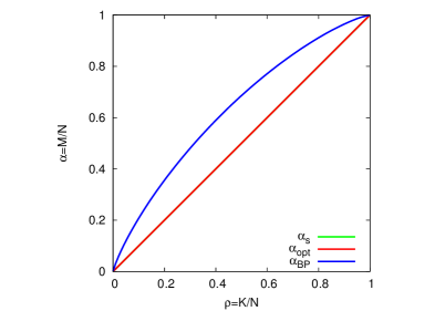
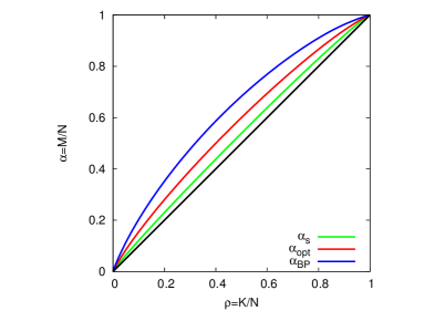
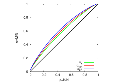
Figure 6: Phase diagram in the plane density $\rho$ measurement rate $\alpha$, with variance of small components $\epsilon=0$ (left), $\epsilon=10^{-6}$ (center) and $\epsilon=10^{-4}$ (right).

In Fig. 6 we plot the phase diagram for fixed variance $\epsilon$ in the density $\rho$ - measurement rate $\alpha$ plane. The only space for improvement is in the region $\alpha_{\rm opt}<\alpha<\alpha_{\rm BP}$. In this region, G-AMP is not optimal because the potential $\Phi(E)$ has two maxima, and the iterations are blocked in the “wrong” local maximum of the potential $\Phi(E)$ with the largest $E$. This situation is well known in physics as a first order transition, with a blocking of the dynamics in a metastable state.

IV Reconstruction of approximately sparse signals with optimality achieving matrices

A first order phase transition that is causing a failure (sub-optimality) of the G-AMP algorithm appears also in the case of truly sparse signals [3]. In that case [3] showed that with the so-called “seeding” or “spatially coupled” measurement matrices the G-AMP algorithm is able to restore asymptotically optimal performance. This was proven rigorously in [4]. Using arguments from the theory of crystal nucleation, it was argued heuristically in [3] that spatial coupling provides improvement whenever, but only if, a first order phase transition is present. Spatial coupling was first suggested for compressed sensing in [9] where the authors tested cases without a first order phase transition (see Fig. 3), hence no improvement was observed. Here we show that for measurement rates $\alpha_{\rm opt}<\alpha<\alpha_{\rm BP}$ seeding matrices allow to restore optimality also for the inference of approximately sparse signals.

IV-A Seeding sampling matrices

The block measurement matrices $F_{\mu i}$ that we use in the rest of this paper are constructed as follows: The $N$ variables are divided into $L_{c}$ equally sized groups. And the $M$ measurements are divided into $L_{r}$ groups of $M_{\rm seed}$ measurements in the first group and $M_{\rm bulk}$ in the others. We define $\alpha_{\rm seed}=L_{c}M_{\rm seed}/N$ and $\alpha_{\rm bulk}=L_{c}M_{\rm bulk}/N$. The total measurement rate is

$$\alpha=\frac{\alpha_{\rm seed}+(L_{r}-1)\alpha_{\rm bulk}}{L_{c}}$$ (19)

The matrix $F$ is then composed of $L_{r}\times L_{c}$ blocks and the matrix elements $F_{\mu i}$ are generated independently, in such a way that if $\mu$ is in group $q$ and $i$ in group $p$ then $F_{\mu i}$ is a random number with zero mean and variance $J_{q,p}/N$. Thus we obtain a $L_{r}\times L_{c}$ coupling matrix $J_{q,p}$. For the asymptotic analysis we assume that $N\to\infty$ and $\alpha_{\rm seed}$, $\alpha_{\rm bulk}$ are fixed. Note that not all block matrices are good seeding matrices, the parameters have to be set in such a way that seeding is implemented (i.e. existence of the seed and interactions such that the seed grows). The coupling measurement matrix $J_{q,p}$ that we use in this paper is illustrated in Fig. 7.

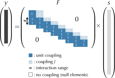
Figure 7: Sketch of the measurement matrices we used to approach optimal reconstruction with the G-AMP algorithm. We use a number of variable-blocks $L_{c}$, and $L_{r}$ measurement blocks. The matrix components are iid with zero mean and variance $1/N$ for the blocks on the diagonal and for a number $W$ of lower diagonals, the upper diagonal blocks have components with variance $J/N$.

To study the state evolution for the block matrices we define $E_{p}^{t}$ to be the mean-squared error in block $p$ at time $t$. The $E_{p}^{t+1}$ then depends on $\hat{m}_{p}^{t}$ from the same block according to eq. (16), on the other hand the quantity $\hat{m}_{p}^{t}$ depends on the MSE $E^{t}_{q}$ from all the blocks $q=1,\dots,L_{c}$ as follows

$$\hat{m}_{p}^{t}=\frac{\alpha_{\rm seed}J_{1p}}{\sum_{q=1}^{L_{c}}J_{1q}E_{q}^{t}}+\alpha_{\rm bulk}\sum_{r=2}^{L_{r}}\frac{J_{rp}}{\sum_{q=1}^{L_{c}}J_{rq}E_{q}^{t}}$$ (20)

This kind of evolution belongs to the class for which threshold saturation (asymptotic achievement of performance matching the optimal Bayes inference solver) was proven in [22] (when $L_{c}\to\infty$, $W\to\infty$ and $L_{c}/W\gg 1$). This asymptotic guarantee is reassuring, but one must check if finite $N$ corrections are gentle enough to be able to perform compressed sensing close to $\alpha_{\rm opt}$ even for practical system sizes. We hence devote the next section to numerical experiments showing that the G-AMP algorithm is indeed able to reconstruct close to optimality with seeding matrices.

IV-B Restoring optimality

In Fig. 8 we show the state evolution compared to the evolution of the G-AMP algorithm for system size $N=6\cdot 10^{4}$. The signal was of density $\rho=0.2$ and $\epsilon=10^{-6}$, the parameters of the measurement matrix are in the second line of Table I, the $L_{c}=30$ giving measurement rate $\alpha=0.303$ which is deep in the region where G-AMP for homogeneous measurement matrices gives large MSE (for $\alpha<0.356$). We see finite size fluctuations, but overall the evolution corresponds well to the asymptotic curve.

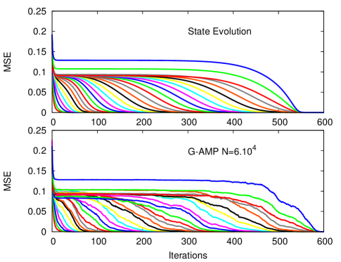
Figure 8: Evolution of the MSE in reconstruction of signal with density $\rho=0.2$, variance of small components $\epsilon=10^{-6}$ at measurement rate $\alpha=0.303$. The state evolution on the top is compared to the evolution of the algorithm for a signal size $N=6\cdot 10^{4}$ on the bottom. The measurement is performed using a seeding matrix with the following parameters: $\alpha_{\rm seed}=0.4$, $\alpha_{\rm bulk}=0.29$, $W=3$, $J=0.2$, $L_{c}=30$.

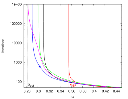
Figure 9: The convergence time of BP for large system sizes estimated by the state evolution as a function of measurement rate $\alpha$. Data are for signals with density $\rho=0.2$, variance of small components $\epsilon=10^{-6}$. The red line is obtained using an homogeneous measurement matrix, the vertical dashed line corresponds to the limit this approach can achieve $\alpha_{\rm BP}=0.3554$. All the other lines are obtained using seeding matrix with parameters specified in Table I and varying $L_{c}$, the resulting measurement rate $\alpha$ is computed from eq. (19). With these seeding matrices and using large $L_{c}$, reconstruction is possible at least down to $\alpha_{\rm bulk}=0.282$ which is very close to the measurement rate $\alpha_{\rm opt}=0.2817$. The blue point corresponds to the evolution illustrated in Fig. 8.

color	$\alpha_{\rm seed}$	$\alpha_{\rm bulk}$	$J$	$W$	$L_{r}$
violet	$0.4$	$0.282$	$0.3$	$3$	$L_{c}+2$
blue	$0.4$	$0.290$	$0.2$	$3$	$L_{c}+1$
green	$0.4$	$0.302$	$0.001$	$2$	$L_{c}+1$
black	$0.4$	$0.310$	$0.4$	$3$	$L_{c}+1$

TABLE I: Parameters of the seeding matrices used in Fig. 9

In Fig. 9 we plot the convergence time needed to achieve reconstruction with $E\approx\epsilon$ for several sets of parameters of the seeding matrices. With a proper choice of the parameters, we see that we can reach an optimal reconstruction for values of $\alpha$ extremely close to $\alpha_{\rm opt}$. Note, however, that the number of iterations needed to converge diverges as $\alpha\to\alpha_{\rm opt}$. This is very similar to what has been obtain in the case of purely sparse signals in [3, 4].

Finally, it is important to point out that this theoretical analysis is valid for $N\to\infty$ only. Since we eventually work with finite size signals, in practice, finite size effects slightly degrade this asymptotic threshold saturation. This is a well known effect in coding theory where a major question is how to optimise finite-length codes (see for instance [23]). In Fig. 10 we plot the fraction of cases in which the algorithm reached successful reconstruction for different system sizes as a function of the number of blocks $L_{c}$. We see that for a given size as the number of blocks is growing, i.e. as the size of one block decreases, the performance deteriorates. As expected the situation improves when size augments. Analyses of the data presented in Fig. 10 suggest that the size of one block that is needed for good performance grows roughly linearly with the number of blocks $L_{c}$. This suggests that the probability of failure to transmit the information to every new block is roughly inversely proportional to the block size. We let for future work a more detailed investigation of these finite size effects. The algorithm nevertheless reconstructs signals at rates close to the optimal one even for system sizes of practical interest.

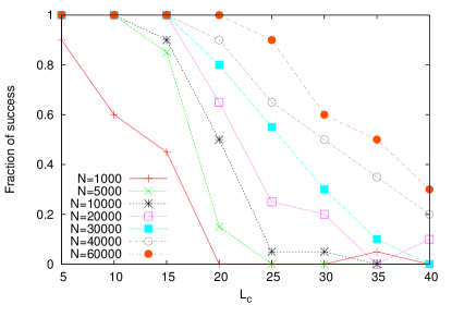
Figure 10: Fraction of instances (over $20$ attempts) that were solved by the algorithm in less than twice the number of iterations predicted by the density evolution for different system sizes, as a function of the number of blocks $L_{c}$. We used the parameters that lead to the blue curve in Fig. 9 (i.e. second line of Table I). As $N\to\infty$, reconstruction is reached in all the instances, as predicted by the state evolution. For finite $N$, however, reconstruction is not reached when $L_{c}$ is too large.

V Discussion

V-A Mismatching signal model

In this paper we treated signals generated by the two-Gaussian model and we assumed knowledge of the parameters used for the generation. Note, however, that in the same way as in [3, 24, 7] the corresponding parameters ($\rho$, $\epsilon$, etc.) can be learned using expectation maximization. For real data it is also desirable to use a signal model (1) that is matching the data in a better way.

At this point we want to state that whereas all our results do depend quantitatively on the statistical properties of the signal, the qualitative features of our results (e.g. the presence and nature of the phase transitions) are valid for other signals, distinct from the two-Gaussian case that we have studied here, and even for the case when the signal model does not match the statistical properties of the actual signal. This was illustrated e.g. for the noisy compressed sensing of truly sparse signal in [7]. In the same line, we noticed and tested that if G-AMP corresponding to $\epsilon=0$ is run for the approximately sparse signals the final MSE is always larger than the one achieved by G-AMP with the right value of $\epsilon$.

We tested the G-AMP algorithm with the signal model (1) and EM learning of parameters on some real images and we indeed observed better performance than for the G-AMP designed for truly sparse signals. However, to become competitive we also need to find better models for the signal, likely including the fact that the sparse components are highly structured for real images. We let this for future work.

V-B Presence of noise

In this paper we studied the case of noiseless measurements, but the measurement noise can be straightforwardly included into the analysis as in [7] where we studied the phase diagram in the presence of the measurement noise. The results would change quantitatively, but not qualitatively.

V-C Computational complexity

The G-AMP algorithm as studied here runs in $O(MN)$ steps. For dense random matrices this cannot be improved, since we need $MN$ steps to only read the components of the matrix. Improvements are possible for matrices that permit fast matrix operations, e.g. Fourrier or Gabor transform matrices [25]. Again, testing approximate sparsity in this case is an interesting direction for future research. Note, however, that the state evolution and replica analysis of optimality does not apply (at least not straightforwardly) to this case.

Another direction to improve the running time of G-AMP is to sample the signal with sparse matrices as e.g. in [8]. For sparse matrices G-AMP is not anymore asymptotically equivalent to the belief propagation (even though it can be a good approximation), and the full belief propagation is much harder to implement and to analyze. But despite this difficulty, it is an interesting direction to investigate.

V-D Spatial coupling

For small variance of the small components of the signal the G-AMP algorithm for homogeneous matrices does not reach optimal reconstruction for measurement rates close to the theoretical limit $\alpha_{\rm opt}$. The spatial coupling approach, resulting in the design of seeding matrices, improves significantly the performance. For diverging system sizes optimality can be restored. We show that significant improvement is also reached for sizes of practical interest. There are, however, significant finite size effect that should be studied in more detail. The optimal design of the seeding matrix for finite system sizes (as studied for instance in depth in the context of error correcting codes [23]) remains an important open question.

References

- [1] E. J. Candés and T. Tao, “Near-Optimal Signal Recovery From Random Projections: Universal Encoding Strategies?” IEEE Trans. Inform. Theory, vol. 52, p. 5406, 2006.
- [2] D. L. Donoho, “Compressed sensing,” IEEE Trans. Inform. Theory, vol. 52, p. 1289, 2006.
- [3] F. Krzakala, M. Mézard, F. Sausset, Y. Sun, and L. Zdeborová, “Statistical physics-based reconstruction in compressed sensing,” Phys. Rev. X, vol. 2, p. 021005, 2012.
- [4] D. L. Donoho, A. Javanmard, and A. Montanari, “Information-theoretically optimal compressed sensing via spatial coupling and approximate message passing,” 2011, arXiv:1112.0708v1 [cs.IT].
- [5] D. Donoho, A. Maleki, and A. Montanari, “Message passing algorithms for compressed sensing: I. motivation and construction,” in Information Theory Workshop (ITW), 2010 IEEE, 2010, pp. 1 –5.
- [6] S. Rangan, “Generalized approximate message passing for estimation with random linear mixing,” in IEEE International Symposium on Information Theory Proceedings (ISIT), 31 2011-aug. 5 2011, pp. 2168 –2172.
- [7] F. Krzakala, M. Mézard, F. Sausset, and L. Z. Yifan Sun, “Probabilistic reconstruction in compressed sensing: Algorithms, phase diagrams, and threshold achieving matrices,” 2012, arXiv:1206.3953v1 [cond-mat.stat-mech].
- [8] D. Baron, S. Sarvotham, and R. Baraniuk, “Bayesian compressive sensing via belief propagation,” IEEE Transactions on Signal Processing, vol. 58, no. 1, pp. 269 – 280, 2010.
- [9] S. Kudekar and H. Pfister, “The effect of spatial coupling on compressive sensing,” in Communication, Control, and Computing (Allerton), 2010, pp. 347–353.
- [10] D. Guo and C.-C. Wang, “Asymptotic mean-square optimality of belief propagation for sparse linear systems,” Information Theory Workshop, 2006. ITW ’06 Chengdu., pp. 194–198, 2006.
- [11] S. Rangan, “Estimation with random linear mixing, belief propagation and compressed sensing,” in Information Sciences and Systems (CISS), 2010 44th Annual Conference on, 2010, pp. 1 –6.
- [12] D. L. Donoho, A. Maleki, and A. Montanari, “Message-passing algorithms for compressed sensing,” Proc. Natl. Acad. Sci., vol. 106, no. 45, pp. 18 914–18 919, 2009.
- [13] D. J. Thouless, P. W. Anderson, and R. G. Palmer, “Solution of ‘solvable model of a spin-glass’,” Phil. Mag., vol. 35, pp. 593–601, 1977.
- [14] M. Bayati and A. Montanari, “The dynamics of message passing on dense graphs, with applications to compressed sensing,” IEEE Transactions on Information Theory, vol. 57, no. 2, pp. 764 –785, 2011.
- [15] D. Guo and C.-C. Wang, “Random sparse linear system observed via arbitrary channels: A decoupling principle,” Proc. IEEE Int. Symp. Inform. Th., Nice, France, pp. 946–950, 2007.
- [16] Y. Wu and S. Verdu, “Optimal phase transitions in compressed sensing,” 2011, arXiv:1111.6822v1 [cs.IT].
- [17] S. Rangan, A. Fletcher, and V. Goyal, “Asymptotic analysis of map estimation via the replica method and applications to compressed sensing,” arXiv:0906.3234v2, 2009.
- [18] D. Guo, D. Baron, and S. Shamai, “A single-letter characterization of optimal noisy compressed sensing,” in 47th Annual Allerton Conference on Communication, Control, and Computing, 2009. Allerton 2009., 2009, pp. 52 – 59.
- [19] A. Jimenez Felstrom and K. Zigangirov, “Time-varying periodic convolutional codes with low-density parity-check matrix,” Information Theory, IEEE Transactions on, vol. 45, no. 6, pp. 2181 –2191, 1999.
- [20] S. Kudekar, T. Richardson, and R. Urbanke, “Threshold saturation via spatial coupling: Why convolutional ldpc ensembles perform so well over the bec,” in Information Theory Proceedings (ISIT),, 2010, pp. 684–688.
- [21] ——, “Spatially coupled ensembles universally achieve capacity under belief propagation,” 2012, arXiv:1201.2999v1 [cs.IT].
- [22] A. Yedla, Y.-Y. Jian, P. S. Nguyen, and H. D. Pfister, “A simple proof of threshold saturation for coupled scalar recursions,” 2012, arXiv:1204.5703v1 [cs.IT].
- [23] A. Amraoui, A. Montanari, and R. Urbanke, “How to find good finite-length codes: from art towards science,” European Transactions on Telecommunications, vol. 18, no. 5, pp. 491–508, 2007. [Online]. Available: http://dx.doi.org/10.1002/ett.1182
- [24] J. P. Vila and P. Schniter, “Expectation-maximization bernoulli-gaussian approximate message passing,” in Proc. Asilomar Conf. on Signals, Systems, and Computers (Pacific Grove, CA), 2011.
- [25] A. Javanmard and A. Montanari, “Subsampling at information theoretically optimal rates,” 2012, arXiv:1202.2525v1 [cs.IT].