Slow motion of internal shock layers for the Jin-Xin system in one space dimension
Abstract.
This paper considers the slow motion of the shock layer exhibited by the solution to the initial-boundary value problem for a scalar hyperbolic system with relaxation. Such behavior, known as metastable dynamics, is related to the presence of a first small eigenvalue for the linearized operator around an equilibrium state; as a consequence, the time-dependent solution approaches its steady state in an asymptotically exponentially long time interval. In this contest, both rigorous and asymptotic approaches are used to analyze such slow motion for the Jin-Xin system. To describe this dynamics, we derive an ODE for the position of the internal transition layer, proving how it drifts towards the equilibrium location with a speed rate that is exponentially slow. These analytical results are also validated by numerical computations.
MARTA STRANI111 Université Paris-Diderot (Paris 7), Institut de Mathématiques de Jussieu, E-mail address: strani@dma.ens.fr, martastrani@gmail.com
Key words. Metastability, slow motion, internal layers, relaxation systems.
1. Introduction
The slow motion of internal shock layers has been recently widely studied. Such phenomenon, known as metastability, is usually related to the presence of a first small eigenvalue for the linearized operator around a given equilibrium state. From a general point of view, a metastable behavior appears when solutions exhibit a first time scale in which they are close to some non-stationary state for an exponentially long time before converging to their asymptotic limit. As a consequence, two different time scales emerge: a first transient phase where a pattern of internal shock layers is formed in a time scale, and a subsequent exponentially slow motion where the layers drift toward their asymptotic limits.
A large class of evolution PDEs, concerning many different areas, exhibits this behavior. Among others, we include viscous shock problems (see [13], [24], [25]), phase transition problems described by the Allen-Cahn equation, with the fundamental contributions [5], [9], and Cahn-Hilliard equation, studied in [1] and [23].
In this paper we mean to study the slow motion of the shock layer for the scalar hyperbolic system with relaxation
| (1.1) |
where the space variable belongs to a one-dimensional interval , . System (1.1) is a particular case of a class of more general hyperbolic relaxation systems of the form
usually utilized to model a variety of non equilibrium processes in continuum mechanics: for example, non-thermal equilibrium gas dynamics ([15], [19]), traffic dynamics ([2], [16], [18]), and multiphase flows ([3], [4], [21]). Here is a positive parameter, usually small, determining relaxation time.
In the case of system (1.1), the parameter can be seen as a viscosity coefficient; we are interested in studying the behavior of the solution to (1.1) in the limit of small , and we want to identify the role of this parameter in the appearance and/or disappearance of phenomena of metastability.
The main example we have in mind is the initial-boundary value problem for the quasilinear Jin-Xin system in the bounded interval , with Dirichlet boundary conditions, that is
| (1.2) |
for some , and flux function that satisfies
| (1.3) |
We stress that, once the boundary conditions for the function are chosen, the boundary conditions for the function are univocally determined. This model was firstly introduced in [10] as a numerical scheme approximating solutions of the hyperbolic conservation law . System (1.2) is strictly hyperbolic, with the spectrum of the Jacobian composed by two distinct real eigenvalues .
In the relaxation limit (), system (1.2) can be approximated to leading order by
| (1.4) |
that is
| (1.5) |
together with , and complemented with boundary conditions
| (1.6) |
From the standard theory of entropy solutions to first-order quasi-linear equations of hyperbolic type, it is known that (1.5) admits a class of solutions, hence possible discontinuous, with speed of propagation given by the Rankine-Hugoniot condition
where denotes the jump. Assumptions (1.3) guarantee that the jump from the value to the value is admissible if and only if , and its speed of propagation is equal to zero. In this case, equation (1.5) admits a large class of stationary solutions satisfying the boundary conditions, given by all that piecewise constant functions in the form
where is a certain point in the interval. Hence, given , we can construct a one-parameter family of steady states, parametrized by that represents the location of the jump, and given by
| (1.7) |
where denotes the characteristic function of the interval . We remark that, once is chosen, the class of stationary solutions for the original system (1.4) is given by the relation , so that
| (1.8) |
For the initial-boundary value problem (1.5)-(1.6), it is possible to prove that every entropy solution converges in finite time to an element of the family . This stabilization property has been proved for the first time in [17], using the theory of generalized characteristic, firstly introduced in [6]. In this framework, assumptions (1.3) on the flux function are crucial (see [20, Theorem 6.1]). Hence, every entropy solution to the initial-boundary value problem
converges in finite time to an element of the family .
For , the situation is very different. If we differentiate with respect to the second equation of (1.2), we obtain
| (1.9) |
Thus, stationary solutions to (1.2) solve
| (1.10) |
together with . The presence of the Laplace operator has the effect that only a single stationary state is admitted (see [12]). As an example, we consider the case of Burgers flux, i.e. , . We can explicitly write the stationary solution for the problem (1.10)-(1.6) as
| (1.11) |
where is implicitly defined by imposing the boundary conditions Moreover, is defined by .
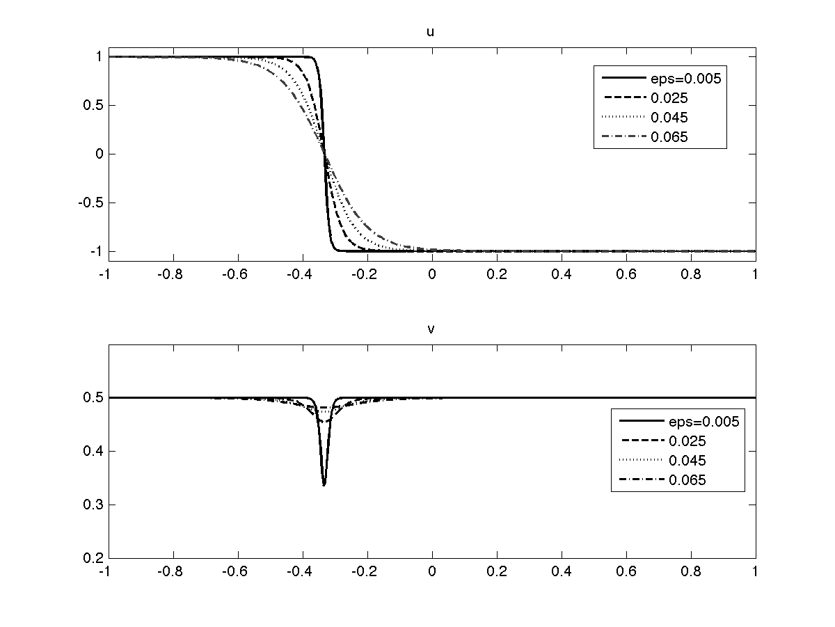
In the limit , the single steady state converges pointwise to , while, for a class of general that verify hypotheses (1.3), the stationary solution converges pointwise to , for some .
Finally, the single steady state is asymptotically stable (for more details see the spectral analysis performed in Section 3), i.e. starting from an initial datum close to the equilibrium configuration, the time dependent solution approaches the steady state for .

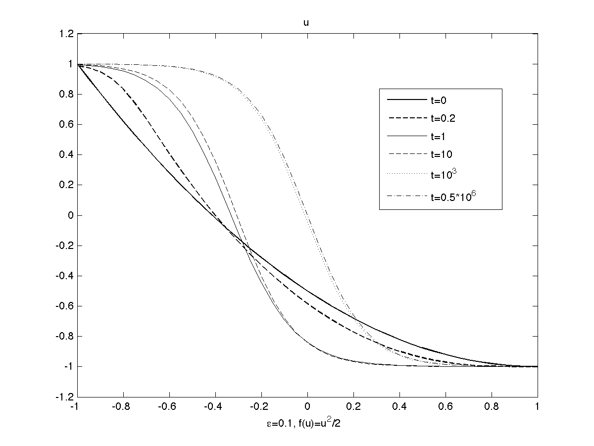
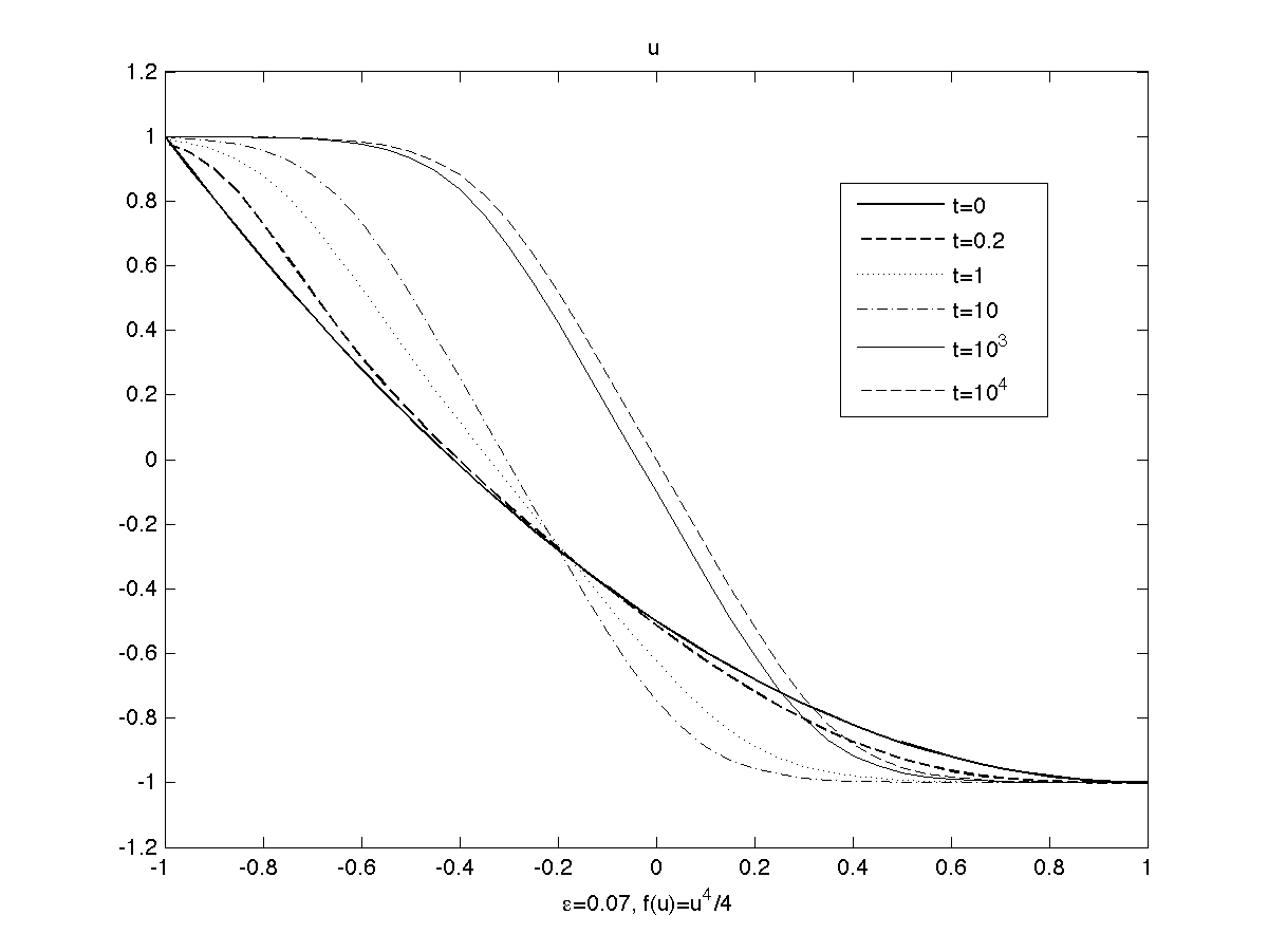
Next question is what happens to the dynamics generated by an initial datum localized far from the equilibrium solution . Numerical computations show that, starting, for example, with a decreasing initial datum (see Fig.1), because of the viscosity, a shock layer is formed in a time scale. More precisely, the solution generated by such initial datum still presents a smooth transition from to , but the shock is located far away from zero, so that the solution is approximately given by a translation of the (unique) stationary solution of the problem. Once the shock layer is formed, it moves towards the equilibrium solution, and this motion is exponentially slow. Thus we have a first transient phase where the shock layer is formed, and an exponentially long time interval where the shock layer approaches the equilibrium solution.
Concerning the function , starting with the initial datum , we can observe that the position of the shock of corresponds to the location of the minimum value of the function ; so we have a first transient phase in which the profile of stabilizes, and an exponentially slow phase where the value of the minimum of such profile drifts towards the value that represents the location of the equilibrium solution for .
The aim of this paper is to study the dynamics generated by an initial datum localized far from the equilibrium solution and to determine a detailed description of the low-viscosity behavior of the solutions.
To the best of our knowledge, the problem of the slow motion for the hyperbolic-parabolic Jin-Xin system (1.1) has been never investigated before. However, system (1.2) can be reduced by differentiation to (1.9) together with the equation , and, as stressed, the study of stationary solutions to (1.9) is the same of that of the scalar conservation law
| (1.12) |
together with the additional condition .
A pioneering article that analyzes the dynamics of (1.12) for initial data close to the equilibrium solution has been published by G. Kreiss and H.O. Kreiss [12]. Here the flux function is given by , so that equation (1.12) becomes the so-called viscous Burgers equation. To study the dynamics generated by such initial configurations, the authors consider the linearized equation close to the unique stationary state defined in (1.11) , that is
In [12] it is shown that, if , the eigenvalues of are all real and negative. Moreover
This precise distribution shows that the large time behavior of solutions is described by terms of order , so that the convergence to the asymptotically stable state is exponentially slow, when is small.
Concerning the phenomenon of metastability for equation (1.12), such problem has been examined, among others, in [24] and in [14]. Here the different approaches are based either on projection method or on WKB expansion, but the common aim is to derive an equation for the position of the shock layer , considered as a function of time, that describes its slow motion towards the equilibrium location. In both papers, the analysis is carried on at a formal level and numerically validated.
A rigorous analysis has been performed firstly in [7] (and generalized to the case of non-convex flux in [8]). There, to study the slow motion of the internal layer, a one-parameter family of functions that approximate the stationary solution is chosen as a family of traveling waves with small velocity.
The phenomenon of metastability for the equation (1.12) has been analyzed by C. Mascia and M. Strani in [20]. To study the problem of the slow motion, the authors introduce a one-parameter family of functions , approximating a stationary solution .
Hence, considering the linearized equation around , it is shown that the eigenvalues of the linearized operator verify, for all
| (1.13) |
Moreover, the position of the shock layer satisfies , where . This estimate shows that the shock layer drifts toward the equilibrium solution with a speed rate proportional to the first eigenvalue , so that this motion is exponentially slow.
Motivated by the analogies among the study of our problem and some results for the scalar conservation law (1.12), in this article we follow the approach presented in [20].
– We build-up a one parameter family of approximate steady states
such that for some , and with the additional property that as in an appropriate sense. Moreover we require the error
to be small in in a sense to be specified. – We describe the dynamics of the system in a neighborhood of the family .
Once a set of reference states is chosen, we determine spectral properties of the linearized operator around such element; moreover we show that, under appropriate hypotheses on how far is an element of the family of approximate steady states from being an exact stationary solution, a metastable behavior appears.
The main difference with respect to [20] is that here we deal with an hyperbolic system. Hence, since the linearized operator around the reference state is not necessarily self-adjoint, we have to consider the chance of having complex eigenvalues, and the spectral analysis need much more care. This paper is organized as follows.
In Section 2 we propose a construction for the family in the case of the Jin-Xin system. Then, we write the solution as
Hence we use as new coordinates the position of the shock layer , and the perturbation . The couple turns to solve an ODE-PDE coupled system of equations. We then study and approximation of such system, obtained by linearizing with respect to and by keeping the nonlinear dependence on , so that the -terms can be neglected.
In Section 3, we analyze spectral properties of the linear operator arising from the linearization around : we show that the spectrum of can be decomposed into three parts: the first eigenvalue is real, negative and , , hence small as ; all the other real eigenvalues are of order ; all the remaining eigenvalues are complex with real and imaginary part less than , . Such estimates show that all of the components relative to all of the eigenvectors except the first one have a very fast decay for small , so that a slow motion occurs as a consequence of the size of the first eigenvalue.
In Section 4, following the idea of [24], we give a precise asymptotic expression for the first eigenvalue of , showing that it is exponentially small for .
Finally, in Section 5, by using the spectral analysis performed in the previous Sections, we analyze the system for the couple ; our main result is Theorem 5.2, where we prove the following estimate for the -norm of the perturbation
| (1.14) |
for some constants and independent on , and where the terms , and are small in in a sense that will be specified in details later on. Precisely, the perturbation has a very fast decay in time, up to a reminder that is bounded by and , hence small in .
Estimate (1.14) can be used to decouple the system for the variables . This leads us to the statement of Proposition 5.4, providing a precise estimate for the variable . In particular, we will show that the shock layer position drifts towards the equilibrium location at a speed rate that becomes smaller as .
Finally, we numerically compute the position of the shock layer at various time, showing that numerical results agree with the analytical results.
2. General Framework
Let us consider the Jin-Xin system
| (2.1) |
for some flux function chosen so that assumptions (1.3) hold. System (2.1) can be rewritten as
| (2.2) |
where
We are interested in studying the behavior of the solution to (2.2) in the relaxation limit, i.e. . We assume that there exists a one-parameter family of functions
such that for some , where is the exact steady state of the system.
When , an element of this family can be seen as an approximate stationary solution to the problem, i.e. as in an appropriate sense to be specified. Moreover we require that, in the relaxation limit, , where and are defined in (1.7)-(1.8).
Let us stress that, once the one-parameter family of functions is chosen, the couple is univocally determined by the relation
Example 2.1.
In the case of Burgers flux, i.e. , a stationary solution to (2.1) satisfies
| (2.3) |
with boundary conditions , for some . An approximate solution to the first equation of (2.3) is obtained by matching two different steady states satisfying, respectively, the left and the right boundary conditions together with the request (see [20, Example 2.1]). In formula
| (2.4) |
where , and are chosen so that the boundary conditions are satisfied
| (2.5) |
Moreover, by the condition , we have
2.1. The linearized problem
As already stated before, in order to describe the dynamics generated by an initial configuration localized far from the steady state , we assume to have a one-parameter family
parametrized by , such that the couple is an approximate stationary solution to (2.1), in the sense that it satisfies the stationary equation up to an error that is small in . More precisely, following the idea firstly introduced in [20], we assume that there exist two families of smooth functions and , uniformly convergent to zero as , such that, for any , the following estimates hold
| (2.6) | ||||
Once a one-parameter family satisfying (2.6) is chosen, we look for a solution to (2.1) in the form
Thus we describe the dynamics in a neighborhood of the family using as coordinates the parameter and a distance vector , determined by the difference between the solution and an element of the approximate family. Substituting in (2.1), we obtain
Since , we get
| (2.7) |
where
Example 2.2.
Let us recall the Example 2.1, where we construct an approximate stationary solution for the Jin-Xin system with and . We want to compute in this specific case
From the explicit formula for given in (2.4), we get .
On the other hand, . By direct substitution, we obtain the identity
in the sense of distributions. We also have
In order to determine the behavior of for small , we need an asymptotic description of the values . Following the idea of [20], let us set and . Relation (2.5) becomes
Therefore, the values are both positive and then
that gives the asymptotic representation
| (2.8) |
where l.o.t. denotes lower order terms. Finally
where for some , so that we end up with
| (2.9) |
showing that this term is exponentially small for and it is null when , that corresponds to the equilibrium location of the shock when .
In this case, if we neglect the lower order terms, we can write an asymptotic formula for , that is
| (2.10) |
Also, from (2.9), it follows that the quantity is exponentially small as , uniformly in any compact subset of ; therefore, for any , there exist constants , indipendent on , such that
| (2.11) |
In particular, hypothesis (2.6) is satisfied in the special case of .
We can also numerically compute the limit of the solution for . For fixed , we observe that, as becomes smaller, the transition between and becomes more sharp, while tends to , according to the fact that, in the limit , the solution converges to (see Fig. 2).
Let us go back to the system (2.7). From now on, in order to simplify the presentation, we set and
| (2.12) |
Moreover, we introduce the following notation: if , , then , while if and , then .
Mimicking the approach of [20] let us assume that, for any , the linear operator has a sequence of eigenvalues with corresponding (right) eigenfunctions (for more details see Section 3). Denoting by the eigenfunctions of the corresponding adjoint operator and setting , we impose that the component is identically zero. Indeed, since we will prove that the first eigenvalue is small in the limit , we set an algebraic condition ensuring orthogonality between and , in order to remove the singular part of the operator . Precisely, we impose the first component of the solution to be zero., so that we solve the equation in a subspace where the operator doesn’t vanish.
Thus, denoting by the initial datum for the perturbation, we have
| (2.13) |
so that
Since is the first (left) eigenfunction, there holds , that is
Hence, from (2.13) we get
Since , we have
and we end up with a scalar differential equation for the variable , that is
| (2.14) |
where
Since we are interested in the regime , the equation (2.14) is approximately solved for small . Thus the term is expanded for , yielding
where
Now, for sake of simplicity, let us call . Thus we end up with the nonlinear equation for , which reads
| (2.15) |
where
| (2.16) |
and is defined as in (2.2). Equation (2.15) has to be coupled with the equation for the perturbation . To this end, (2.7) is rewritten in the form
| (2.17) |
Using (2.15), we end up with the following equation
| (2.18) |
where
Hence we obtain the following coupled system for the shock layer location and the perturbation
| (2.19) |
Example 2.3.
Let us consider the Jin-Xin system, for which one obtains
For what concerns the linear operator, setting , and recalling the definition of given in (2.12), we get the following expression for the adjoint operator
complemented with Dirichlet boundary conditions. To obtain an asymptotic expression for the function , we need to approximately compute the functions and . As usual, we refer to the case .
For , the function is close to the eigenfunction of the operator relative to the eigenvalue , with
For example, in we have
that is and , where is an integration constant. By imposing the conditions on the boundary and on the jump, and by doing the same computations in the interval , we obtain
so that for . Furthermore, with the approximation and , we have
so that and converge to and respectively as in the sense of distributions. Thus, since , we deduce an asymptotic expression for the function
With the choice of proposed in Example 2.1, such expression becomes
| (2.20) |
3. Spectral analysis
In this section we analyze the spectrum of the linearized operator in order to determine a precise description of the location of the eigenvalues.
We recall that has been defined in (2.12), so that the eigenvalue problem reads
complemented with Dirichlet boundary conditions. Hence, by differentiating the second equation with respect to , we obtain
| (3.1) |
Then we are interested in studying the eigenvalue problem for the linear differential diffusion-transport operator
| (3.2) |
In [20] it is proven that, under appropriate hypotheses on the behavior of the function in the limit , the eigenvalues of have the following distribution
More precisely, the following Propositions are proven in [20] (for more details, see [20, Proposition 4.1 and Proposition 4.3]).
Proposition 3.1.
Let be a family of functions satisfying the assumption:
A0. There exists a constant , independent on , such that
If there exist , and a constant for which , where is the step function jumping from to , then there exist constants such that .
Proposition 3.2.
Let be a family of functions satisfying the assumptions:
A1. , is twice differentiable at any and
A2. For any there exists such that, for any satisfying , there holds
A3. The left (reps. the right) first order derivatives of at exist and
Then there exists a constant such that, for all , for all sufficiently small.
Remark 3.3.
When , then . With the choice of proposed in Example 2.1, we can easily check that hypotheses A0-1-2-3 are verified.
From (3.1), we observe that is an eigenvalue of if and only if is an eigenvalue for the operator defined in (3.2). Hence, if is an eigenvalue of , then there exists an eigenvalue such that
so that
| (3.3) |
Hence, if , then . Moreover, since are negative for all
| (3.4) |
Due to Propositions 3.1 and 3.2, we know that and as . Thus, from (3.3) and (3.4), there exists a constant such that
Moreover, if for some there exist other eigenvalues such that , then they are of order , so that
On the other hand, if , then . More precisely
Proposition 3.2 assures that there exists such that for all , so that and are terms of order . For example, if and we take into account , the corresponding eigenvalues for verifies
Moreover, for , since , we have
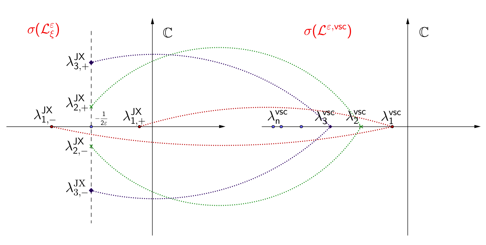
Figure 3 shows the connection between the two spectra when , so that only the first two eigenvalues of belong to .
Hence, the following proposition holds
Proposition 3.4.
Let be a family of functions satisfying assumptions A0-1-2-3 for some and for some . Then the spectrum of the linearized operator can be decomposed as follow i. and . ii. and . iii. There exists such that
iv. for all and
Remark 3.5.
Remark 3.6.
In [12], Kreiss G. and Kreiss H. performed the spectral analysis for the operator
arising from the linearization around the exact steady state of
proving that all the eigenvalues are real and negative. By using this result and our spectral analysis, if we linearize the system (2.1) around the exact stationary solution , we can prove that the real part of all the eigenvalues of the linearized operator is negative, so that the steady state is asymptotically stable with exponential rate.
4. Asymptotic estimates for the first eigenvalue
In this section we want to study the behavior in of the principal eigenvalue of the operator associated to the linearization of (2.1) around an approximate stationary solution. Since usually the metastable behavior is the result of the presence of a first small eigenvalue, our aim is to determine an asymptotic expression for . We have already emphasized the fact that is an eigenvalue of the nonlinear Jin-Xin system if and only if is an eigenvalue for the operator defined in (3.2) where and where is an approximate stationary solution for the scalar conservation law
| (4.1) |
In particular
| (4.2) |
In [20], in the special case , is given by (2.4). In that paper it is proven that, for
so that
| (4.3) |
This formula shows that the principal eigenvalue of the Jin-Xin system with is exponentially small in .
In order to determine an asymptotic expression of the first eigenvalue of the operator (LABEL:opasy) for a general class of flux function , we refer to the paper of Reyna L.G. and Ward M.J., [24]; here the authors use the method of matched asymptotic expansions (MMAE) to determine an approximate stationary solution to (4.1).
Mimicking their approach and performing the same calculations as in [24], with the appropriate changes due to the fact that the study of our equation is made in the interval instead of , we obtain that the leading order MMAE solution for is given by a function , where and the shock profile satisfies
The positive constant and describe the tail behavior of and are defined by
In particular, when , , according to (1.11). Notice that the MMAE solution satisfies exactly the equation, while the boundary conditions are satisfy within exponentially small terms. Instead, the construction presented in this paper in Example 2.1 gives a function that verifies exactly the boundary conditions and solves approximately the stationary equation.
The eigenvalue problem associated to the linearization around is given by
| (4.4) |
In [24] it is proven that the first eigenvalue of (4.4) has the following asymptotic representation (for details see [24, Formula (2.14)])
Finally, from (4.2), we get
| (4.5) |
This formula shows that is exponentially small as . We remark that, when , and , so that (4.5) is the same as (4.3).
5. The behavior of the shock layer position
Let us consider the system (2.19) for the couple and let us neglect the terms
| (5.1) |
This system is obtained by linearizing with respect to and by keeping the nonlinear dependence on , in order to describe the slow motion of the shock layer position far from the equilibrium location .
We complement the so called quasi-linearized system (5.1) with initial data
The aim of this section is to analyze the behavior of the solution to (5.1) in the limit of small . Subsequently, we will prove a result that characterizes the behavior of the shock layer location, proving that it moves towards the unique stationary solution with exponentially small rate.
Before stating our result, let us recall the assumptions.
H1. Let the family be such that there exist two families of smooth functions and such that
We also assume that is asymptotically a solution, i.e. we require that
uniformly with respect to .
Example 2.2 show that hypothesis H1 is verified in the case of the quadratic flux .
H2. There exists a constant such that
By comparing the asymptotic expression for given in (4.3) with the one for and obtained in Example 2.3, we can easily check that hypothesis H2 is verified for the Jin-Xin system when . H3. For what concern the eigenvalues of the linear operator , we have proven that there exist two positive constants independent on such that
H4. Concerning the solution to the linear problem , we require that there exists such that for all , there exist constants and such that
| (5.2) |
Remark 5.1.
The assumption that for all means that the estimate (5.2) holds uniformly in . Since belongs to a bounded interval of the real line, if we suppose that is a continuous function, then there exists a maximum in . For example, in the case of the Jin-Xin system with , the constant behaves like , and the estimate (5.2) is independent of .
5.1. Estimate on the perturbation
Our first aim is to obtain an estimate the perturbation . We recall that
| (5.3) |
where
In particular, is a bounded operator, such that
| (5.4) |
Indeed, if we ask the family to be never transversal to the first eigenfunction of the corresponding linearized operator, we can assume
for some independent on . This gives us a (weak) restriction on the choice of the family .
Concerning the term , we have
| (5.5) |
for some positive constants and independent on and .
For the special case of , both and are bounded by terms that are exponentially small in , while, for a general class of flux functions that verify (1.3), the hypotheses we required assure that all the terms in the equations for the perturbation are small in .
Theorem 5.2.
Let hypotheses H1-4 be satisfied. Then, for sufficiently small, the solution Y to (5.3) satisfies the estimate
for some positive constants , and
Proof.
Since the operator is a linear operator that depends on time, to obtain rigorous estimates on the solution , we need to use the theory of stable families of generators, that is a generalization of the theory of semigroups for evolution systems of the form . We will use some results of [22], which have been summarized in the Appendix A. More precisely, we want to show that is the infinitesimal generator of a semigroup .
To this aim, concerning the eigenvalues of the linear operator , we know that is negative and behaves like for all , so that is such that , and this estimate is independent on . Hence, by using Definition 6.1 and Remark 6.2 (see Appendix A), we know that, for , is the infinitesimal generator of a semigroup , . Furthermore, since (5.2) holds, we get
so that the family is stable with stability constants and . Furthermore, since
Theorem 6.3 (see Appendix A) states that the family is stable with and .
In order to apply Theorem 6.8 (see Appendix A), we need to check that the domain of does not depend on time, and this is true since depends on time through the function , that does not appear in the higher order terms of the operator. More precisely, the principal part of the operator does not depend on . Hence, we can define as the evolution system of , so that
| (5.6) |
Moreover, there holds
Finally, from the representation formula (5.6) with , it follows
| (5.7) |
so that, by using (5.5), we end up with
| (5.8) |
∎
Remark 5.3.
In the special case of Burgers flux, is going to zero exponentially as , since behaves like and from the explicit formula of and in Example 2.2. In the general case, assumptions H1-2 assure that as .
5.2. Slow motion of the shock layer
An immediate consequence of the estimate (5.8) is that, for for some , the function satisfies
More precisely, we can prove the following Proposition.
Proposition 5.4.
Let hypotheses H1-4 be satisfied. Assume also
| (5.9) |
Then, for and sufficiently small, the solution converges to as .
Proof.
Due to the estimate (5.8), for and sufficiently small and for any initial datum , the location of the shock layer satisfies
| (5.10) |
where
More precisely, in the regime of small , the shock location has similar decays properties to those of the solution to the following reduced problem
| (5.11) |
By means of a standard method of separation of variable, we get
Since , by integrating we obtain the following estimate for the shock layer location
| (5.12) |
where represent the equilibrium location for the shock layer position and as . Therefore converges to as , and the convergence is exponential for any under consideration.
∎
Formula (5.12) shows the slow motion of the shock layer for small . Precisely, the evolution of the collocation of the shock towards the equilibrium position is much slower as becomes smaller.
For example, when , and (see formula (2.20)). We also emphasize that hypotheses (5.9) are verified in the case of the Jin-Xin system with .
The following table shows a numerical computation for the location of the shock layer for different values of the parameter and . The initial datum for the function is . We can see that the convergence to is slower as becomes smaller.
The numerical location of the shock layer for different values of the parameter
| TIME | , | , | , | , | , |
|---|---|---|---|---|---|
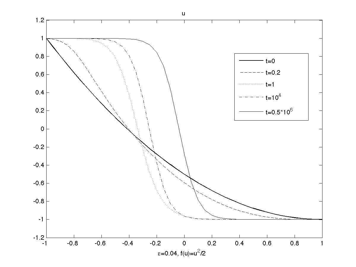
Figure 4 shows the dynamics of the shock layer (i.e the dynamics of the solution to (2.1)), obtained numerically. When , the shock layer location converges to zero very fast: as we can also see from the table, when , the value of is already very close to zero. On the other hand, when becomes smaller the shock layer location moves slower and it approaches the equilibrium location only for very large . Finally, Figure 5 shows the profile of the shock layer for the flux function , that still verifies hypotheses (1.3).

f

6. Appendix A
In this section, we briefly review some results on the theory of evolution systems by A. Pazy [22, Chapter 5]. For more details and for the proofs of the Theorems, see [22, Theorem 2.3, Theorem 3.1, Theorem 4.2].
Let be a Banach space. For every , let be a linear operator in and let be an valued function. Let us consider the initial value problem
| (6.1) |
In the special case where is independent of , the solution to (6.1) can be represented via the formula of variations of constants
where is the semigroup generated by . In [22] it is shown that a similar representation formula is true also when depends on time.
Definition 6.1.
Let a Banach space. A family of infinitesimal generators of semigroups on is called stable if there are constants and (called the stability constants) such that
and
for and for every finite sequence , .
Remark 6.2.
If for , is the infinitesimal generator of a semigroup , satisfying , then the family is clearly stable with constants and .
The previous remark means that, if for every fixed the operator generates a semigroup , and we can find an estimate for that is independent of , then the whole family is stable in the sense of Definition 6.1.
Theorem 6.3.
Let be a stable family of infinitesimal generators with stability constants and . Let , be a bounded linear operators on . If for all , then is a stable family of infinitesimal generators with stability constants and .
In order to prove the existence of the so called evolution system for the initial value problem (6.1), let us introduce two Banach spaces and , with norms , respectively. Moreover, let us assume that is a dense subspace of and that there exists a constant such that for all .
Definition 6.4.
Let be the infinitesimal generator of a semigroup , , on . is called -admissible if it is an invariant subspace of , and the restriction of to is a semigroup on . Moreover, the infinitesimal generator of the semigroup on , denoted here with , is called the part of in .
Next, let us fix , and let be the infinitesimal generator of a semigroup on . The following assumptions are made (H1) is a stable family with stability constants and . (H2) Y is -admissible for and the family is a stable family in with stability constants , . (H3) For , , is a bounded operator from into and in continuous in the norm.
Remark 6.5.
The assumption that the family satisfies (H2) is not always easy to check. A sufficient condition for (H2) which can be effectively checked in many applications states that (H2) holds if there is a family of isomorphisms of onto such that and are uniformly bounded and is of bounded variation in the norm (for more details, see [22, Chapter 5]).
Remark 6.6.
Condition (H3) can be replaced by the weaker condition (H3)’ For , and .
Theorem 6.7.
Let , be the infinitesimal generator of a semigroup , on . If the family satisfies the conditions (H1)-(H3), then there exists a unique evolution system , , in satisfying
| (6.2) |
Moreover, if , the solution to (6.1) can be written as
| (6.3) |
for all .
One special case in which the conditions of Theorem 6.7 can be easily checked is the case where the domain of the operator is independent on . In this case we can take as the Banach space which we denote by , and the following Theorem holds
Theorem 6.8.
Let be a stable family of infinitesimal generators of semigroups on . If is independent on and for , is continuously differentiable in , then there exists a unique evolution system , , satisfying (6.2). Morevoer, if , then, for every , the initial value problem (6.1) has a unique solution given by (6.3).
Acknowledgments
I wish to thank C. Mascia for having introduced me to the problem and for guidance throughout writing the paper.
References
- [1] Alikatos N.D., Bates P.W., Fusco G. (1991). Slow motion for the Cahn-Hilliard equation in one space dimension J. Differential Equations 90, no. 1, 81–135
- [2] Aw A., Rascle M. (2000). Resurrection of ”second order models of traffic flow”, SIAM J. Appl. Math. 60, no. 3, 916–938.
- [3] Beranblatt G.I., Garcia-Azorero J., De Pablo A., Vazquez J.L. (1997). Mathematical model of the non-equilibrium water-oil displacement in porus strata Appl. Anal. 65, no. 1-2, 19–45.
- [4] Barenblatt G.I., Vinnichenko A.P. (1980). Nonequilibrium filtration of nonmixing fluids, Adv. in Mech. 3, no. 3, 35–50.
- [5] Carr J., Pego R. L. (1989). Metastable patterns in solutions of , Comm. Pure Appl. Math. 42, no. 5, 523–576.
- [6] Dafermos C.M. (2005). Hyperbolic Conservation Laws in Continuum Phisics, 2nd. edition, Grundlehren Math. Wiss. 325, Springer-Verlag, Berlin.
- [7] de Groen P. P. N., Karadzhov G. E. ( 1998). Exponentially slow traveling waves on a finite interval for Burgers’ type equation, Electron. J. Differential Equations, No. 30, 38 pp. (electronic).
- [8] de Groen P. P. N., Karadzhov G. E. (2001). Slow travelling waves on a finite interval for Burgers’-type equations, Advanced numerical methods for mathematical modelling. J. Comput. Appl. Math. 132, no. 1, 155–189.
- [9] Fusco G., Hale J. K. (1989). Slow-motion manifolds, dormant instability, and singular perturbations, J. Dynam. Differential Equations 1, no. 1, 75–94.
- [10] Jin S., Xin Z. (1995). The relaxation schemes for systems of conservation laws in arbitrary space dimension Comm. Pure Appl. Math. 48, no. 3, 235–276.
- [11] Kim Y.-J., Tzavaras A. (2001). Diffusive -waves and metastability in the Burgers equation, SIAM J. Math. Anal. 33, no. 3, 607–633 (electronic).
- [12] Kreiss, G., Kreiss, H. (1986). Convergence to steady state of solution of Burgers equation Appl. Numer. Math. 2, no. 3-5, 161–179.
- [13] Laforgue J.G.L., O’Malley Jr R.E. (1994). On the motion of viscous shocks and the supersensitivity of their steady-state limits, Methods Appl. Anal. 1, no. 4, 465–487.
- [14] Laforgue J.G.L., O’Malley Jr R.E. (1995). Shock layer movement for Burgers equation, Perturbations methods in physical mathematics (Troy, NY, 1993). SIAM J. Appl. Math. 55, no. 2, 332–347.
- [15] Levermore D.C. (1996). Moment closure hierachies for kinetic theories, J. Statist. Phys. 83, no. 5-6, 1021–1065.
- [16] Li T. (2000). Global solutions and zero relaxation limit for traffic flow model, SIAM J. Appl. Math. 61, no. 3, 1042–1061
- [17] Liu T.P. (1978). Invariants and asymptotic behavior of solutions of a conservation law, Proc. Amer. Math. Soc. 71, 227–231
- [18] Lighthill M.J., Whitham G.B. (1955). On kinematic waves. II. A theory of traffic flow on long crowded roads, Proc. Roy. Soc. London: Ser. A. 229, 317–345.
- [19] Muller I., Ruggeri T. (1998). Rational extended thermodynamics, Second edition, Springer Tracts in Natural Philosophy, 37, Springer-Verlag, New York.
- [20] Mascia C., Strani M. (2012). Metastability for scalar conservation laws in a bounded domain , submitted.
- [21] Natalini R., Tesei A. (1999). On the Barenblatt model for non-equilibrium two phase flow in porous media, Arch. Ration. Mech. Anal 150, no. 4, 349–367.
- [22] Pazy A. (1983). Semigroups of Linear Operators and Applications to Partial Differential Equations, Applied Mathematical Science 44, Springer-Verlag, New York.
- [23] Pego R.L. (1989). Front migration in the nonlinear Cahn-Hilliard equation, Proc. Roy. Soc. London Ser. A 422, no. 1863, 261–278.
- [24] Reyna L.G., Ward M.J. (1995). On the exponentially slow motion of a viscous shock, Comm. Pure Appl. Math. 48, no. 2, 79–120.
- [25] Sun X., Ward M.J. (1999). Metastability for a generalized Burgers equation with applications to propagating flame fronts, European J. Appl. Math. 10, no. 1, 27–53.