Characterization of coherent structures in three-dimensional turbulent flows using the finite-size Lyapunov exponent

Abstract

In this paper we use the finite size Lyapunov Exponent (FSLE) to characterize Lagrangian coherent structures in three-dimensional (3d) turbulent flows. Lagrangian coherent structures act as the organizers of transport in fluid flows and are crucial to understand their stirring and mixing properties. Generalized maxima (ridges) of the FSLE fields are used to locate these coherent structures.

Three-dimensional FSLE fields are calculated in two phenomenologically distinct turbulent flows: a wall-bounded flow (channel flow) and a regional oceanic flow obtained by numerical solution of the primitive equations where two-dimensional turbulence dominates.

In the channel flow, autocorrelations of the FSLE field show that the structure is substantially different from the near wall to the mid-channel region and relates well to the more widely studied Eulerian coherent structure of the turbulent channel flow. The ridges of the FSLE field have complex shapes due to the 3d character of the turbulent fluctuations.

In the oceanic flow, strong horizontal stirring is present and the flow regime is similar to that of 2d turbulence where the domain is populated by coherent eddies that interact strongly. This in turn results in the presence of high FSLE lines throughout the domain leading to strong non-local mixing. The ridges of the FSLE field are quasi-vertical surfaces, indicating that the horizontal dynamics dominates the flow. Indeed, due to rotation and stratification, vertical motions in the ocean are much less intense than horizontal ones. This suppression is absent in the channel flow, as the 3d character of the FSLE ridges shows.

1 Introduction

Turbulent flow occurs in the natural environmental and in technological applications with such frequency that it could be considered the ”natural” state of fluid flows to be found around us. Traditionally, fluid flows have been observed and studied in the Eulerian perspective where a fixed position is observed for a definite interval of time. The other perspective, the Lagrangian, follows the motion of the fluid and thus is better suited to study aspects of fluid flow such as material transport or the deformation of fluid material in a given state of motion.

The use of stretching quantifiers such as the Lyapunov exponents, which measure the relative separation between particles [1, 2, 3, 4], has broadly improved the Lagrangian study of fluid flows. On the one hand Lyapunov methods provide information on time scales for dispersion processes, with its relevance for mixing and stirring of fluids [1, 2, 3, 5, 6, 7]. On the other, they are useful to detect the so-called Lagrangian coherent structures (LCS). LCSs [8, 9] are templates for particle advection in complex flows, separating regions with different dynamical behavior and acting as barriers and avenues to transport, fronts or eddy boundaries [9, 3, 4, 10, 6, 11, 12, 13].

Relationships of LCSs with Lyapunov fields have been established for the case of finite-time Lyapunov exponents (FTLEs) [14, 15]. These relationships state that LCS can be identified with the ridges (generalized maxima) of the FTLE field. Furthermore they state that the flux through the LCS is inversely proportional to the strength of the ridge and to the integration time of the FTLE field calculation. This flux is shown to be small and the LCS extracted as the ridges of FTLE fields are considered to be almost material-like surfaces. This identification has become widely used in the field although it should be mentioned that there are other more precise definitions of LCS [11, 16, 17], that consider LCS to be exact material surfaces admitting zero flux across them. In our work, we use instead finite-size Lyapunov exponents (FSLEs), which quantify the separation rate of fluid particles between two given distance thresholds [1, 2]. They turn out to be convenient for the case of bounded flows in which characteristic spatial scales are more direct to identify than temporal ones and have been shown to be robust with respect to noisy or poorly resolved velocity fields [18]. Although a rigorous connection between the FSLE and LCSs has not been established yet, previous work [10, 6, 19, 12, 20] has shown that the ridges of the FSLE behave in a similar fashion as the ridges of the FTLE field. Following these works we assume that LCSs can be computed as ridges of FSLEs, and that they are transported by the flow as almost material surfaces/lines, with negligible flux of particles through them. Observations presented here are consistent with those assumptions.

Despite its relevance in real flows, the full three-dimensional (3d) structure of LCSs is still an open subject. In 3d flows, LCS were explored in atmospheric contexts [21, 22, 23], and in a turbulent channel flow at $Re_{\tau}=180$ in [24]. A kinematic ABC flow was studied in [25]. In the ocean, where it is widely recognized that filamental structures, eddies, and in general oceanic meso- and submeso-scale structures have a great influence on marine ecosystems [26, 27, 28, 29], the identification of LCSs and the study of their role in the transport of biogeochemical tracers has primarily been restricted to two-dimensional (2d) layers [30, 31, 32, 33]. There are two concurrent reasons for this: a) because of stratification and rotation, vertical motions in the ocean are usually very small when compared to horizontal displacements; b) synoptic measurements (e.g. from satellites) of relevant quantities are restricted to the surface. A few previous results for Lagrangian eddies in 3d were obtained in Refs. [34, 35], by applying the methodology of lobe dynamics and the turnstile mechanism. Also, Refs. [36, 37] used 3d FSLE fields to identify LCS in oceanic flows. In particular, a mesoscale eddy in the Southern Atlantic was studied in [37], and it was shown that oceanic LCSs presented a vertical curtain-like shape, i.e. they look mostly like vertical sheets, and that material transport into and out of the mesoscale eddy occurred through filamentary deformation of such structures.

In this paper, we use 3d fields of FSLE to identify LCSs in a turbulent channel flow and in an oceanic flow. Observations of the similarities and differences between the two systems, both in their computation and their physical meaning, helps to appreciate the power and scope of this Lagrangian technique in the analysis of fluid flows. In Section 2 we describe the methodology used to identify LCSs in 3d turbulent flows. Sections 3 and 4 are devoted to the turbulent channel flow and the oceanic flow, respectively, and Section 5 presents our conclusions and directions for future work.

2 Methods

2.1 Finite-Size Lyapunov Exponents.

In order to study non-asymptotic dispersion processes such as stretching at finite scales and bounded domains, the finite size Lyapunov Exponent was introduced [1, 2, 3]. It is defined as:

$$\lambda=\frac{1}{\tau}\log\frac{d_{f}}{d_{0}},$$ (1)

where $\tau$ is the time it takes for the separation between two particles, initially $d_{0}$, to reach a value $d_{f}$. In addition to the dependence on the values of $d_{0}$ and $d_{f}$, the FSLE depends also on the initial position of the particles and on the time of deployment. Locations (i.e. initial positions) leading to high values of this Lyapunov field identify regions of strong separation between particles, i.e., regions that will exhibit strong stretching during evolution, that can be identified with the LCS [3, 10, 6].

In principle, to compute FSLE in 3d, the method of [6] can be extended to include the third dimension, by computing the time it takes for particles initially separated by $d_{0}=[(\Delta x_{0})^{2}+(\Delta y_{0})^{2}+(\Delta z_{0})^{2}]^{1/2}$ to reach a final distance of $d_{f}=[(\Delta x_{f})^{2}+(\Delta y_{f})^{2}+(\Delta z_{f})^{2}]^{1/2}$. We will proceed this way for the turbulent channel, but, as indicated in [37], vertical displacements are much smaller than horizontal ones in ocean flows. Therefore, the displacement in the $z$ direction does not contribute significatively to the calculation of $d_{f}$ in the ocean, which prompt us to implement a quasi-3d computation of FSLEs: we use the full 3d velocity field for particle advection but particles are initialized in 2d horizontal ocean layers and the contribution $\Delta z_{f}$ is not considered when computing $d_{f}$ (see more details in [37]). In any case, since we allow the full 3d trajectories of particles, we take into account the vertical dynamics of the oceanic flows.

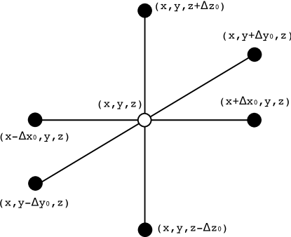
Figure 1: Computational setup for the calculation of the FSLE field in 3d. The FSLE at the location of the central particle (◦) is a measure of the time it takes for any of the neighbor particles (•) to diverge from the central particle by a distance greater than $\delta_{f}$.

Concerning the turbulent channel, where we can implement a fully 3d computation of the FSLE, we proceed as follows. A grid of initial locations $\textbf{x}_{0}=(x_{i},y_{j},z_{k})$ is set up at time $t$, fixing the spatial resolution of the FSLE field (figure 1). Particles are released from each grid point and their three-dimensional trajectories are calculated. The distances of each neighbor particle with respect to the central one (initially $d_{0}$) is monitored until one of the separations reaches a value $d_{f}$.

In both systems considered, we obtain two different types of FSLE maps by integrating the three-dimensional particle trajectories backward and forward in time: the attracting LCSs (for the backward), and the repelling LCSs (forward) [10, 6]. We obtain in this way FSLE fields with a spatial resolution given by $d_{0}$. When a particle leaves the velocity field domain or reaches a no-slip boundary, the FSLE value at its initial position and initial time is set to zero. If the interparticle separation remains smaller than $d_{f}$ past a maximum integration time $\Delta t$, then the FSLE for that location is also set to zero.

2.2 Lagrangian Coherent Structures.

The identification of LCS calculated from Lyapunov fields in 2d flows is straightforward since they practically coincide with (finite-time) stable and unstable manifolds of relevant hyperbolic structures in the flow [8, 9, 10] (but see [38, 16]). The structure of these manifolds in 3d is generally much more complex than in 2d [25, 39], and they can be locally either lines or surfaces.

Differently than 2d, where LCS can be visually identified as the maxima of the FSLE field, in 3d they are hidden within the volume data and one needs to explicitly compute and extract them, using the definition of LCSs as the ridges of the FSLE field. A ridge $L$ is a co-dimension 1 orientable, differentiable manifold (which means that for a 3d domain $D$, ridges are surfaces) satisfying the following conditions [15]:

1. The field $\lambda$ attains a local extremum at $L$.

2. The direction perpendicular to the ridge is the direction of fastest descent of $\lambda$ at $L$.

The method used to extract the ridges from the scalar field $\lambda(\mathbf{x}_{0},t)$ is from [40]. It uses an earlier [41] definition of ridge in the context of image analysis, as a generalized local maxima of scalar fields. For a scalar field $f:\mathbb{R}^{n}\rightarrow\mathbb{R}$ with gradient $\mathbf{g}=\nabla f$ and Hessian $\mathbf{H}$, a d-dimensional height ridge is given by the conditions

$$\forall{d<i\leq n,}\quad\mathbf{g}^{\mathrm{T}}\mathbf{e}_{i}=0\ \textrm{and}\ \alpha_{i}<0,$$ (2)

where $\alpha_{i},i\in\{1,2,\ldots,n\}$, are the eigenvalues of $\mathbf{H}$, ordered such that $\alpha_{1}\geq\ldots\geq\alpha_{n}$, and $\mathbf{e}_{i}$ is the eigenvector of $\mathbf{H}$ associated with $\alpha_{i}$. For $n=3$, Eq. (2) becomes

$$\mathbf{g}^{\mathrm{T}}\mathbf{e}_{3}=0\ \textrm{and}\ \alpha_{3}<0.$$ (3)

In other words, in $\mathbb{R}^{3}$ the $\mathbf{e}_{1},\mathbf{e}_{2}$ eigenvectors point locally along the ridge and the $\mathbf{e}_{3}$ eigenvector is orthogonal to it, so the ridge maximizes the scalar field in the normal direction to it and in this direction the field is more convex than in any other direction, since the eigenvector associated with the most negative eigenvalue is oriented along the direction of maximum negative curvature of the scalar field.

The extraction process progresses by calculating the points where the ridge conditions are verified and the ridge strength $|\alpha_{3}|$ is higher than a predefined threshold $s$ so that ridge points whose value of $\alpha_{3}$ is lower (in absolute value) than $s$ are discarded from the extraction process. Since the ridges are constructed by triangulations of the set of extracted ridge points, the strength threshold greatly determines the size and shape of the extracted ridge, by filtering out regions of the ridge that have low strength. The reader is referred to [40] for details about the ridge extraction method. The height ridge definition has been used to extract LCS from FTLE fields in several works (see, among others, [42]).

Since the $\lambda$ value of a point on the ridge and the ridge strength $\alpha_{3}$ are only related through the expressions (2) and (3), the relationship between the two quantities is not direct, which makes difficult to choose the appropriate strength threshold $s$. A too small value of $s$ will result in the extraction of very small LCSs that appear to have little influence on the dynamics, while a large value will result in only a partial rendering of the larger and more significant LCS, limiting the possibility of observing their real impact on the flow.

The ridges extracted from the backward FSLE map approximate the attracting LCSs, and the ridges extracted from the forward FSLE map approximate the repelling LCSs. The attracting ones are the more interesting from a physical point of view [6, 12], since particles (or any passive scalar driven by the flow) typically approach them and spread along them, so that they are good candidates to be identified with the typical filamentary structures observed in tracer advection.

3 Turbulent channel flow

Turbulent channel flow is a turbulent flow between two stationary, parallel walls separated by a distance $2\delta$. It has been studied extensively due to its geometrical simplicity and its wall-bounded nature, which makes it a suitable platform to study phenomena appearing in more complex turbulent wall-bounded flows of great technological interest.

The coordinates of the flow are: $x$ for the streamwise direction, $y$ for the cross-stream coordinate that separates the two plates, and $z$ for the spanwise direction. The flow is maintained by a downstream pressure gradient $\frac{dP_{0}}{dx}$ acting against the wall shear stress. The laminar flow solution $U_{0}$ is a cross-stream parabolic profile given by

$$U_{0}(y)=\frac{y^{2}-\delta^{2}}{2\mu}\frac{dP_{0}}{dx}\ ,$$ (4)

where $\mu$ is the dynamic viscosity. Following the Reynolds averaging method [43], the turbulent flow velocity $\mathbf{u}$ is decomposed in a mean $\mathbf{U}=(U(y),0,0)$ and a fluctuating component $\mathbf{u}^{\prime}=(u^{\prime},v^{\prime},w^{\prime})$. The mean turbulent velocity profile $U(y)$ differs from the laminar one, $U_{0}(y)$, by a lower centerline velocity $U(0)$ and increased near-wall velocity giving it a flatter shape. Due to the increase in mean velocity near the wall, the shear stress near the wall is higher for the turbulent case. The total shear stress $\tau$ appearing in the averaged Reynolds equations gets contributions from both the viscous stress and the Reynolds stress $-\overline{u^{\prime}v^{\prime}}$ associated to the velocity fluctuations:

$$\frac{\tau}{\rho}=\nu\frac{dU}{dy}-\overline{u^{\prime}v^{\prime}}$$ (5)

$\nu={\mu}/{\rho}$ is the kinematic viscosity. The symmetries of the domain and the Reynolds equations imply that $\tau$ depends only on the cross-stream coordinate $y$, and the dependence is linear, so that it can be written as

$$\frac{\tau(y)}{\rho}=u_{\tau}^{2}\left(1-\frac{y}{\delta}\right)$$ (6)

The shear velocity $u_{\tau}$ gives the velocity scale of the turbulent velocity fluctuations. The formula [43]:

$$\rho u_{\tau}^{2}=\mu\left.\frac{dU(y)}{dy}\right|_{y=0}$$ (7)

allows to compute $u_{\tau}$ from measurements of the mean velocity profile from the simulations. A length scale can be formed by combining $u_{\tau}$ with $\nu$: the wall scale $\delta^{+}={\nu}/{u_{\tau}}$. The wall distance can now be expressed as $y^{+}=y/\delta^{+}$, and the same normalization could be done for the rest of coordinates. The viscous Reynolds number $Re_{\tau}={\delta}/{\delta^{+}}$ is simply the ratio between the two relevant length scales.

The existence of coherent structures in turbulent wall-bounded flows has been known for several decades from investigations on intermittency in the interface between turbulent and potential flow regions, on the large eddy motions in the outer regions of the boundary layer, and on coherent features in the near-wall region ([44] and references therein). Since then, through experimental and numerical investigations, a picture of the organization of these coherent structures in the turbulent boundary layer has emerged, which has become rather complete from the Eulerian point of view [44, 45]. Our approach is a contribution to the Lagrangian exploration of these coherent structures, as in [24] and [46].

The longitudinal velocity field in the inner region of the channel (the viscous sublayer adjacent to the wall and the intermediate buffer region) is organized into alternating streamwise streaks of high and low speed fluid. Turbulence production occurs mainly in the buffer region in association with intermittent and violent outward ejections of low-speed fluid and inrushes of high-speed fluid towards the wall. The outer region is characterized by the existence of three-dimensional $\delta$-scale bulges that form on the turbulent/potential flows interface. Irrotational valleys appear at the edges of the bulges, entraining high-speed fluid into the turbulent inner region. A central element in the structure of the turbulent boundary layer is the hairpin vortex, mainly because it is a structure with the capability of transporting mass and momentum across the mean velocity gradient and because it provides a paradigm with which to explain several observations of wall turbulence [44, 47].

3.1 Data

The data used to extract the LCS come from a direct numerical simulation (DNS) of turbulent channel flow at a viscous Reynolds number $Re_{\tau}=180$. The setup of the simulation follows that of [48] and is summarized in table 1. The simulations were conducted using the CFD solver Channelflow.org [49]. The Channelflow.org code solves the incompressible Navier-Stokes equations in a rectangular box with dimensions $L_{x}\times 2\delta\times L_{z}$, with periodic boundary conditions in the $x$ (so that fluid leaving the computational domain in the direction of the mean flow at $x=L_{x}$ reenters it at $x=0$) and in the spanwise $z$ direction. No-slip conditions are imposed on $y=\pm\delta$. The unsteady velocity field $\bf{u}$ is represented as a combination of Fourier modes in the $x$ and $z$ directions and of Chebyshev polynomials in the wall-normal direction. The pressure gradient necessary to balance the friction at the walls was chosen as to maintain a constant bulk velocity of $\frac{2}{3}U_{0}$. Time stepping is a 3rd-order Semi-implicit Backward Differentiation. Note that in our computations $\delta^{+}=1/Re_{\tau}=0.0058$ so that in wall units $0<y^{+}<344$.

The flow was integrated from an initial base-flow with parabolic profile and a small disturbance that evolved into a fully developed turbulent flow. The total integration time was $\Delta t=600$ time units that in dimensionless form $t^{+}=t\left(u_{\tau}^{2}/\nu\right)$ gives $\Delta t^{+}=83.54$. After an initial transient of about $200$ time units the simulations reached a statistically stationary state from which statistics was accumulated.

The mean quantities and first order statistics of our simulations where compared to those of [48] and the agreement is quite good. The profile of the mean velocity in wall units is shown in figure 2. The profile for the Reynolds stress $-\overline{u^{\prime}v^{\prime}}$ shows that the maximum (in absolute value) is located at approximately $y^{+}=30$, in the outer limit of the buffer layer (see figure 3).

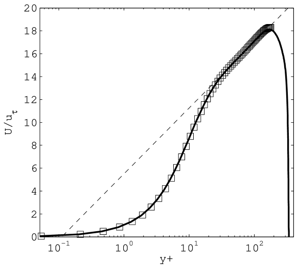
Figure 2: Mean velocity profile $U(y)/u_{\tau}$ . Solid line: our simulations; squares: [48]; dashed line: logarithmic profile $U(y)/u_{\tau}=2.5\log(y^{+})+5.5$.

Figure 3: Reynolds stress $\overline{u^{\prime}v^{\prime}}$ profile at $Re_{\tau}=180$. Solid line: our simulations; squares: [48] (given up to the channel centerline).

Table 1: Simulation parameters. Quantities with ⁺ refer to wall units. $L_{x}$, $2\delta$ and $L_{z}$ are the domain sizes in the $x$, $y$ and $z$ directions. $\Delta x^{+}$, $\Delta y^{+}$ and $\Delta z^{+}$ are the respective spatial resolutions (given at the first point above the wall for the $y$ case), and $n_{x}$, $n_{y}$ and $n_{z}$ the corresponding number of grid points. $Re=U\delta/\nu$ is the Reynolds number based on the channel center mean speed, whereas $Re_{\tau}=u_{\tau}\delta/\nu$ is the viscous Reynolds number. The nominal value is an input to the computer code, and the actual value comes by using Eq. (7) for the computed mean profile $U(y)$.

• $Re$ channel center	$4000$	$Re_{\tau}$ nominal	$180$	$Re_{\tau}$ actual	$172$
  $L_{x}$	$4\pi$	$\delta$	$1$	$L_{z}$	$\frac{4}{3}\pi$
  $L_{x}^{+}$	$2166.61$	$\delta^{+}$	$0.0058$	$L_{z}^{+}$	$722.20$
  $n_{x}$	128	$n_{y}$	129	$n_{z}$	128
  $\Delta x^{+}$	$17.06$	$\Delta y^{+}$	$0.005$	$\Delta z^{+}$	$5.6867$

3.2 Results

The LCS were extracted from the turbulent velocity field data described in the previous section. A calculation of FSLE field in the entire turbulent channel was conducted in order to understand the statistical properties of the FSLE field in this class of turbulent flows. A subsequent calculation in a subdomain of the channel was used to extract the LCS in that subdomain for a sequence of time instants. The setup of both calculations is shown in table 2.

Table 2: FSLE calculation parameters. $dt$ is the integration time step and $\Delta t$ the maximum integration time.

• Calculation	$d_{0}$	$d_{f}/d_{0}$	$\Delta t$	$dt$
  Complete channel	$0.024$	$20$	$20$	$0.05$
  LCS subdomain	$0.003$	$67$	$10$	$0.05$

3.2.1 The 3d FSLE field.

The 3d backward FSLE field for the entire channel was calculated at a single time instant in the statistically steady state. The initial and final distances $d_{0}$ and $d_{f}$ were chosen as a balance between encompassing the widest possible range of scales of motion (measured by the ratio $d_{f}/d_{0}$), and adequate resolution and computational cost. The initial distance is of the order of $4\delta^{+}$ and the final distance of the order of $0.5\delta$ – a typical scale of coherent structures found in the turbulent channel flow – so that the ratio of scales, $d_{f}/d_{0}$, is approximately $Re_{\tau}/8$.

Figure 4: Instantaneous FSLE field at $t=420$ shown on a streamwise/wall-normal plane in the turbulent channel. Walls are at the top and bottom of the figure. Mean velocity is in the streamwise direction from left to right.

Figure 5: FSLE profile averaged over $(x,z)$, as a function of the cross-stream normalized coordinate $y^{+}$. Only half of the channel is shown since the profile is quasi-symmetric about the channel centerline.

Figure 4 shows an instantaneous configuration of the FSLE values in a streamwise/wall-normal plane. The maxima of the FSLE appear to be located close to the walls with ocasional sloping structures extending to the midchannel region. The channel center is devoid of high FSLE values but coherent patches of low FSLE values can still be observed. These structures are not distributed uniformly along the length of the channel but appear to be organized in packets. This organization bears resemblance to the widely accepted picture of organized structures in wall turbulence where the outer region is dominated by packets of sloping hairpin vortices and the inner region by near wall vortices (the hairpin vortices legs) and shear layers [47, 44].

A cross-stream FSLE profile is obtained by averaging the 3d field over the periodic directions $x$ and $z$. It is shown in figure 5. The profile is symmetric about the channel centerline and shows a maximum at approximately $y^{+}=4$, inside the viscous sublayer (this location corresponds to the first grid point off the wall).

Because of the periodic boundary conditions in the $x$ and $z$ directions the average profiles along these directions are rather unstructured, and we resort to two-point correlation functions to quantify the statistical structure properties. For each plane parallel to the walls, i.e. for each value of $y^{+}$, we compute the fluctuations of the FSLE values around the average in that plane: $\Lambda(x^{+},y^{+},z^{+})\equiv\lambda(x^{+},y^{+},z^{+})-\left<\lambda(x^{+},y^{+},z^{+})\right>_{x^{+},z^{+}}$. From this quantity we define the streamwise $R_{xx}(y^{+};\bar{x}^{+})$ correlation function as:

$$R_{xx}(y^{+};\bar{x}^{+})=\frac{\left<\Lambda(x^{+},y^{+},z^{+})\Lambda(x^{+}+\bar{x}^{+},y^{+},z^{+})\right>_{x^{+},z^{+}}}{\left<\Lambda(x^{+},y^{+},z^{+})^{2}\right>_{x^{+},z^{+}}}\ ,$$ (8)

and the spanwise $R_{zz}(y^{+};\bar{z}^{+})$ correlation function

$$R_{zz}(y^{+};\bar{z}^{+})=\frac{\left<\Lambda(x^{+},y^{+},z^{+})\Lambda(x^{+},y^{+},z^{+}+\bar{z}^{+})\right>_{x^{+},z^{+}}}{\left<\Lambda(x^{+},y^{+},z^{+})^{2}\right>_{x^{+},z^{+}}}\ .$$ (9)

In the above equations the averages are over the periodic directions $x^{+}$ and $z^{+}$. The correlations are shown in Figs. 6 and 7 at different distances from the walls: one smaller, one larger, and one approximately coincident with the location of the maximum Reynolds stress. These functions reveal sizes and organization of the different structures in the Lagrangian FSLE field, to be contrasted with Eulerian correlation functions in the same system [50].

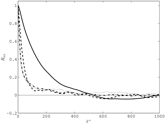
Figure 6: Streamwise correlation function $R_{xx}(y^{+};\bar{x}^{+})$ as a function of the streamwise separation $\bar{x}^{+}$, at four distances from the lower wall: Continuous line: $y^{+}=4$; dashed line $y^{+}=12.2$; dash-dot line $y^{+}=28.4$; dotted line: $y^{+}=122.1$.

Figure 7: Spanwise correlation function $R_{zz}(y^{+};\bar{z}^{+})$ as a function of the spanwise separation $\bar{z}^{+}$, at four distances from the lower wall: Continuous line: $y^{+}=4$; dashed line $y^{+}=12.2$; dash-dot line $y^{+}=28.4$; dotted line: $y^{+}=122.1$.

Close to the wall ($y^{+}=4$ and $y^{+}=12.2$), viscous effects dominate. The correlations show that the FSLE field is organized in streamwise structures of length scale approximately $l^{+}\sim 500$ wall units. In the transverse direction $z^{+}$ the oscillations seen in $R_{zz}$ for $y^{+}=4$ indicate an approximately periodic arrangement of the streaks [24], with a spacing $\sim 50-100$ wall units. This pattern of organization is similar to what is seen in Eulerian descriptions [50, 44].

At planes further away from the wall ($y^{+}=28.4$ and $y^{+}=122.1$ in Figs. 6 and 7), correlation functions in both directions become shorter ranged, and periodic features are progressively lost. This corresponds to a rather disordered distribution of structures, each with a typical size related to the width of the correlation functions, i.e. of the order of 50 wall units, as also seen in figure 4.

An instantaneous near-wall FSLE field is shown in figure 8, where the high FSLE values appear in slender and elongated structures with length and width corresponding to the streamwise and spanwise correlation lengths discussed above. It is unclear whether the correlation lengths result from a single streamwise structure or from the overlaping of shorter structures (a feature of the near wall coherent structure arrangement [51]).

These are the highest FSLE values that are to be found in the channel as the plot in figure 5 shows. The mechanism for the formation of these structures could be the lifting of low speed fluid close to the wall by the action of counter rotating vortex pairs located above the viscous sublayer (see figure 9). This mechanism is widely known in the Eulerian view of coherent structures of turbulent wall bounded flows (ejections or bursting, [47]).

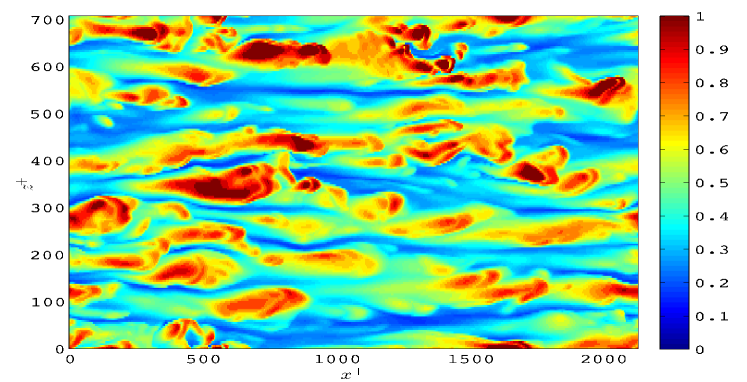
Figure 8: Instantaneous FSLE field in plane parallel to the wall at $y^{+}=4$. The time is the same as in figure 4

Figure 9: Mechanism for the rapid separation of fluid from the near wall viscous sublayer. The mean flow is into the page.

The near wall fluid is advected away from the wall by the action of these vortices. This mechanism could be responsible for very fast particle separation in particle pairs where one particle is lifted away and the other remains in the low speed zone close to the wall. We note that the particle separation would increase not only by the wall normal distance between particles but also because the ejected particle would move to a region with higher streamwise velocity. Shear layers near the wall is another possible way to produce large particle dispersion. These mechanisms would explain the fact that the maximum average FSLE is located so close to the wall and not on the buffer region where turbulence production is larger. To conclude, we note that these high FSLE regions near the wall seem to extend to the midchannel region in an inclined fashion. It is not clear whether this pattern signals the existence of a hairpin vortex with streamwise legs and inclined head or if there are two separate structures: the streamwise vortices and the hairpin arch or head [44]. Also, we note that the interpretation of the high FSLE regions near the wall do not require the existence of a counter rotation pair of vortices, as only one vortex would suffice.

To illustrate these mechanisms, a map of the FSLE field in a spanwise/wall normal plane for the LCS domain calculation is shown in figure 10, together with a set of passive particles initially located in a rectangular region close to the wall and released some instants before the time of the FSLE map. In order to focus just on the above mentioned ejection mechanism involving only the vertical motion of the particles, the trajectory integration was made in a 2d fashion by setting the longitudinal component of the particles velocity to zero.

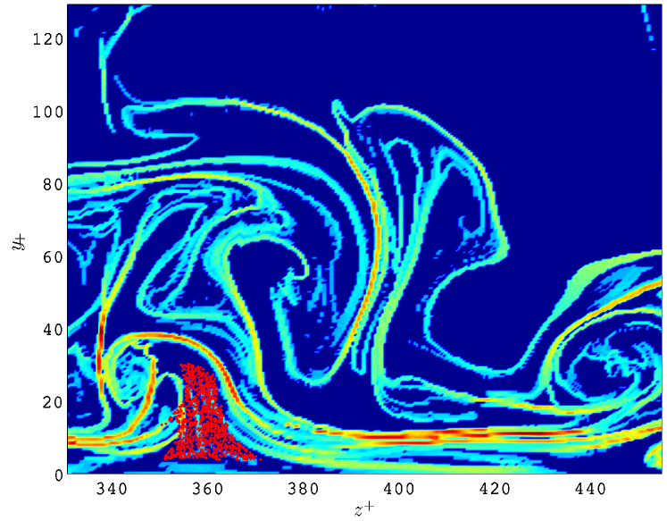
Figure 10: FSLE map in a $(z,y)$ plane located at $x=6.0$ ($x^{+}=1034$). The time of the map is $t=413.8$. together with a set of particles initially located in rectangular region $z^{+}\in[345,380]$ and $y^{+}\in[3.4,13.8]$. The particles were released at $t=409$. Particle trajectories were integrated using only the spanwise and wall normal velocity components. The mean flow is moving out of the page.

The particles seem to have been lifted from wall by a streamwise vortex located to the left of the particle plume, with center at $(z^{+},y^{+})\sim(340,30)$. We note that the structures are moving with the mean flow and that the continuous motion of the particles away from the wall is due to the passage of a streamwise structure that imparts this sustained motion to the particles for long enough time. To compare the Eulerian and Lagrangian coherent structures, figure 11 shows the turbulent velocity components in the same plane at the nearest time available in the turbulent dataset. The signature of the streamwise vortex discussed above can be seen in the Eulerian map at the same location. It is embedded in a patch of negative streamwise velocity fluctuation $u$. To the right, close to $z^{+}=380$, a vertical shear layer appears dividing the negative and positive patches of $u$. The Lagrangian signature of this vertical shear layer is not very strong and appears in figure 10 as quasi-vertical line of moderate FSLE extending from $y^{+}=25$ to $y^{+}=60$. On the lower right of the map, there is a set of high FSLE lines almost parallel to wall, signalling the existence of high particle dispersion. In the Eulerian map (figure 11), it can be seen that there is a shear layer parallel to the wall at the same location ($400<z^{+}<440$ and $y^{+}\sim 8$). The fact that this shear layer has a much stronger Lagrangian signature than the vertical shear layer could be because it has the same orientation and sign of the mean shear and therefore acts together with the latter to disperse neighboring particles across the wall normal direction. The high FSLE line seen at the middle of the map in figure 10, separating the two convoluted features can be seen to be related to the existence of two counter-rotating vortices, one with center located at $\sim(380,60)$ and the other at $\sim(420,100)$. The line of high FSLE line is seen to be located at the boundary between both vortices. In section 3.2.3, we present a 3d view of these structures and their evolution in time.

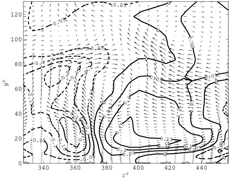
Figure 11: Instantaneous turbulent velocity components at $x=6.0$ ($x^{+}=1034$) and $t=413.75$. Velocity vectors correspond to the inplane velocity components $(w,v)$, together with contours of streamwise turbulent velocity $u$. Dashed contours are negative $u$ (into the paper) and continuous countours are positive $u$ (from the paper).

3.2.2 Propagation velocity.

In turbulent channel flow the velocity perturbations propagate in the streamwise direction aproximately with the velocity of the mean flow[52]. In the case of Lyapunov exponents, [46] measured the FTLE field in an 2D turbulent boundary layer velocity field obtained by time-resolved PIV measurements. The FTLE maxima were found to move with the mean flow velocity.

We measured the propagation velocity of the FSLE field perturbation using a space-time correlation of the form:

$$R_{uu}(y^{+};\bar{x}^{+};\bar{t}^{+})=\frac{\left<\Lambda(x^{+},y^{+},z^{+},t^{+})\Lambda(x^{+}+\bar{x}^{+},y^{+},z^{+},t^{+}+\bar{t}^{+})\right>_{x^{+},z^{+}}}{\left<\Lambda(x^{+},y^{+},z^{+},t^{+})^{2}\right>_{x^{+},z^{+}}}\ ,$$ (10)

where $\bar{x}^{+}$ and $\bar{t}^{+}$ are the delays in the streamwise direction and time. The time delay is fixed and the propagation velocity is defined as

$$V^{+}=\frac{\bar{X}^{+}}{\bar{t}^{+}}\ ,$$ (11)

where $\bar{X}^{+}$ is the streamwise lag for which $R_{uu}$ is maximum. The choice of the time delay is related to the time scale of the FSLE field. A first rule is to choose a time delay that gives reasonable peaks in the correlation. If there are several time scales present, several $\bar{t}^{+}$ will result in correlations exhibiting peaks. The calculation of (11) was made for a full length and height spanwise section of the channel. A time series of FSLE fields with time step of $dt^{+}=1.8$ and time length $\Delta t^{+}=431$ was calculated for this section to offset the effects of the limited spanwise extent of the section. The final time lag used in (11) was equal to $dt^{+}$. All larger delays produced correlations with no significant peak. A reason for this could be the fact that by setting the FSLE final distance the length scales of turbulence retained in the FSLE field is fixed, and then there will be only one time delay producing a peak in the correlation (10), specifically that corresponding to $V^{+}$.

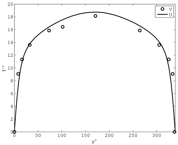
Figure 12: Propagation velocity of FSLE field ($V^{+}$) and mean flow ($U^{+}$).

The profile of the propagation velocity is shown in figure 12. The propagation velocity is very close to the mean flow velocity. The result shows that the maxima of the FSLE field, that produce high values of $R_{uu}$ and where we expect to find the ridges of the FSLE field, move with the flow. Hence, one may conclude, as expected, that the FSLE ridges also move with the flow approximately as material surfaces.

3.2.3 The 3d LCS.

The previous description summarized the statistical properties of the different structures appearing in an instantaneous FSLE field. To make further progress we now extract three-dimensional attracting LCSs in a region of the channel at a series of time instants. The extraction domain had dimensions $L_{x}^{+}\times L_{y}^{+}\times L_{z}^{+}=103\times 129\times 124$. The initial separation $d_{0}$ and distance ratio $d_{f}/d_{0}$ were increased from the previous calculation to improve the resolution and extract smoother structures, but sacrificing a complete view of 3d LCS in the turbulent channel. The extraction threshold was set to $s=50000$, a compromise value between speed and cost of extraction and continuity of the extracted surfaces. The FSLE fields were calculated for an interval of $1.5$ time units with a time step of $0.1$ units.

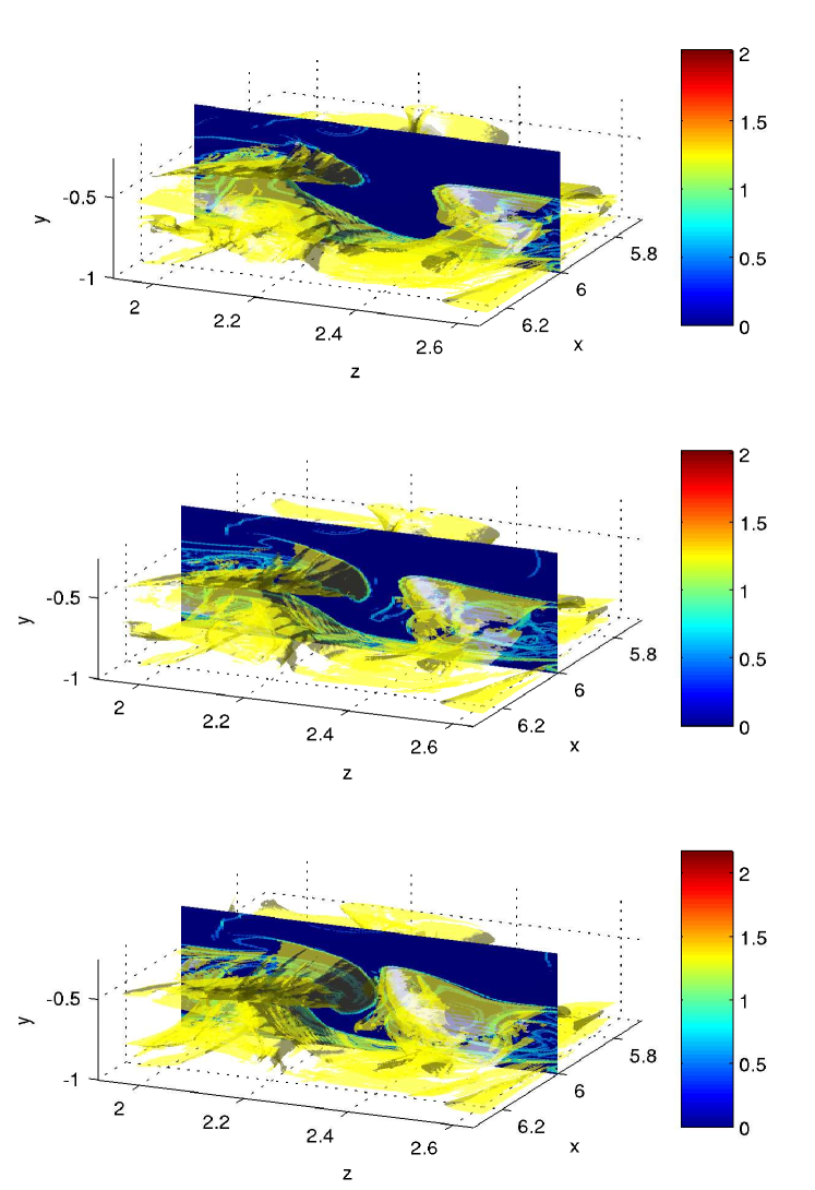
Figure 13: 3d attracting LCS in the channel flow together with a FSLE map at the fixed plane $x=6.0$ ($x^{+}=1034$). Time goes from top to bottom, at intervals of 0.1 time units. The flow direction is in the positive $x$ direction in each panel, and a wall is at the bottom. The sequence shows how one of the flow structures is advected and passes through the $x=6.0$ plane.

The 3d LCSs are rendered in figure 13, in a sequence of time instants, as they pass through the calculation domain. They have a clearly 3d shape and move with the flow. The LCS seem to create a boundary between the inner turbulent region and the outer region that is practically devoid of FSLE. The highest LCS have $\delta$-scale heights above the wall, and have a distinct mushroom shape enclosing the regions of the channel closer to the wall, where high FSLE values can be found. Near the wall, the LCS adopt the shape of sheets parallel to it, which reflects the high rates of shear that occur in that region. These sheets form the base of the mushroom-shaped excursions up to the channel center.

4 Oceanic flow

Contrarily to the turbulent flow of the previous section, large scale oceanic flows, naturally turbulent, can be considered as almost 2d due to rotation and stratification effects. This fact makes the theory of 2d turbulence a very important tool to understand the ocean processes that occur at large scales. The main characteristic of 2d turbulence is the existence of an inverse energy cascade, from the small to the large scales and a direct enstrophy cascade. These cascades manifests themselves by the creation of large coherent vortices, and by the process of filamentation by which strain regions in the boundaries of the vortices produce lines of vorticity that are continuously stretched and deformed by the flow, concentrating the vorticity gradient in the small scales. This behavior is often observed in oceanic flows thereby confirming the importance of the 2d turbulent processes.

The results presented in this section were obtained in the Benguela ocean region, situated off the west coast of southern Africa. It is characterized by a substantial mesoscale activity in the form of eddies and filaments, and also by the northward drift of Agulhas eddies. The velocity data set comes from a regional ocean model (ROMS) simulation of the Benguela Region [53]. Additional details on this work can be found in [37].

The three-dimensional FSLE fields were calculated for a $30$ day period starting September 17 of year 9, with snapshots taken every $2$ days. The fields were calculated for an area of the Benguela ocean region between latitudes 20°S and 30°S and longitudes 8°E to 16°E. The calculation domain extended vertically from $20$ up to $580$ m of depth. Both backward and forward calculations were made in order to extract the attracting and repelling LCS.

In the left panel of figure 14 a snapshot of the attracting LCSs for day 1 of the calculation period is shown. The structures appear as thin vertical curtains, most of them extending throughout the whole depth of the calculation domain. The horizontal slices of the FSLE field in figure 14 (left panel) show that the attracting LCS fall on the maximum FSLE field lines, as in the case of the turbulent channel flow (figure 13). The FSLE fields themselves exhibit a variation in intensity that decreases with depth, altough a local maximum is found at $\sim 100$ m (not shown). The ridges also seem to be weaker as the depth increases since for the same strength threshold, the extracted portions of the ridges become less extent and eventually vanish. The atracting and repelling LCS (figure 14, right panel) populate the calculation region, testifying the enhanced mixing activity that is known to occur in that particular ocean region. The quite entangled “web” in which attracting and repelling LCSs intersect mutually provides the skeleton for the barriers and pathways controlling transport [6, 11].

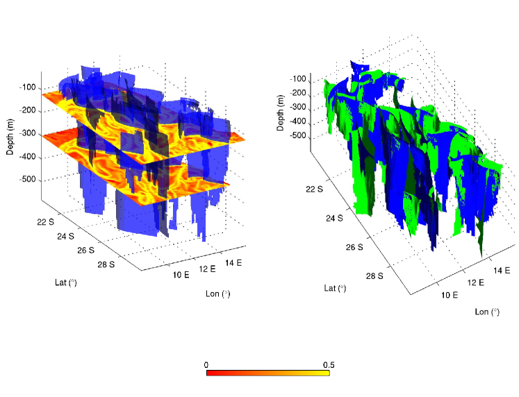
Figure 14: 3d LCS in the Benguela region for day 1 of the calculation period. Left panel (from [37]): Attracting LCS together with horizontal slices of the backward FSLE field at 120 m and 300 m depth. Right panel: Attracting (blue) and repelling (green) LCS. Colorbar refers to colormap of horizontal slices in the left panel. The units of the colorbar are $day^{-1}$.

At this point, it may help to stress the differences between the Eulerian and Lagrangian detection of coherent structures. This can be seen in figure 15 where the boundaries of a mesoscale eddy are shown using the Q-criterion and the attracting and repelling LCS. The Q-criterion [54] uses the second invariant of $\nabla\mathbf{u}$:

$$Q=\frac{1}{2}(\|\mathbf{\Omega}\|^{2}-\|\mathbf{S}\|^{2}),$$ (12)

where $\|\mathbf{\Omega}\|^{2}=\textrm{tr}(\mathbf{\Omega}\mathbf{\Omega}^{\mathrm{T}})$, $\|\mathbf{S}\|^{2}=\textrm{tr}(\mathbf{S}\mathbf{S}^{\mathrm{T}})$, and $\mathbf{\Omega}$, $\mathbf{S}$ are the antisymmetric and symmetric components of $\nabla\mathbf{u}$, to identify regions where rotation dominates strain ($Q>0$), commonly identified with coherent vortices, and strain dominated regions ($Q<0$). We refer the reader to [55] and [56] for reviews and criticism of several Eulerian criteria.

Eulerian and Lagrangian measures limit approximately the same region, but are substantially different. The Q-criterion is related to the instantaneous configuration of the second invariant of $\nabla\mathbf{u}$ and therefore conveys only local information about fluid flow processes. The Lagrangian perspective, on the other hand, provides an integration of the temporal evolution of material properties of the flow, e.g. material transport, and thus should give more meaningful information about the processes that rely on ocean material transport.

This issue can be further explored by looking at a filamentation event (described more extensively in [37]). A set of particles were released inside the eddy at day 1 at a depth of 50 m. At day 11 of the calculation period (see figure 15), they have formed a filament that is expelled from the eddy, so that particles clearly cross the Q-criterion isosurface. This shows that the Eulerian criteria is inadequate as an indicator of regions of material transport in the flow. On the contrary, it can be observed that the Lagrangian description of the eddy boundaries does bear relation with material transport into and out of the eddy, since the particle filament leaves the enclosed region that we associate with the mesoscale eddy by following one of the identified Lagrangian boundaries.

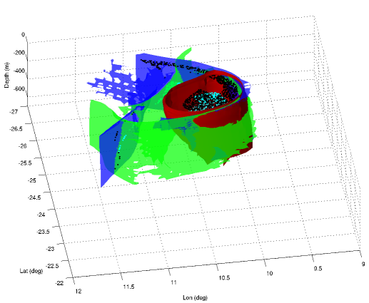
Figure 15: Attracing (blue) and repelling (green) LCS on day 11 of the calculation period together with Q-criterion isosurface at $Q=10^{-10}$ (red). The particles (black dots) were released inside the eddy at day 1 at a depth of 50 m and are leaving now the eddy as a filament along the upper part of the attracting LCS.

5 Conclusions

Lyapunov exponents are useful to identify Lagrangian coherent structures in turbulent flows. These constitute the pattern determining the pathways of particle transport in the flow and thus strongly influence the transport and mixing properties in the fluid.

In this paper we have used a particular type of Lyapunov exponents, the so-called Finite-Size Lyapunov exponents, to identify LCS in 3d flows. The finite size Lyapunov exponent was used to measure the rate of streching of initially nearby fluid particles in the flow domain and the Lagrangian coherent structures where identified as the the ridges of the FSLE field. These ridges were filtered in order to retain only the strongest attracting or repelling structures.

In a turbulent channel flow, the FSLE field is organized into longitudinal structures close to the wall that develop into sloping ones away from the wall. Correlations in the streamwise and spanwise direction show the typical dimensions of these structures. They were found to be similar to the Eulerian coherent structures that are known to exist in this same regions of the turbulent channel. Specially, elongated streamwise vortices that move low speed fluid away from the wall into the channel core. In 3d, the LCSs appear as mushroom-shaped excursions of near-wall sheet-like structures of a scale comparable to the channel width. They separate the channel into an interior region, where the FSLE attains high values, and an exterior region, showing low FSLE values. The distribution of LCS in the turbulent channel resembles the commonly accepted picture where upward excursions of near wall fluid coexist with inward rushes of mid-channel irrotational flow. Further work is necessary to elucidate the relations between LCS and fluid transport in these type of flows, not least because the visualization of 3d structures and transport in turbulence is a complex and time-consuming subject.

In a quasi-2d mesoscale oceanic flow, the LCSs appear as quasi-vertical surfaces highlighting the fact that dispersion in this case is mainly horizontal. The high mixing activity can be deduced from the proliferation of LCS in the flow domain and their mutual intersection. These LCS were seen to provide barriers and pathways to transport in the case of a mesoscale eddy, contrary to Eulerian measures that failed to provide indicative locations or directions of major transport events.

The main difference between these two 3d turbulent flows with respect to the LCSs seems to be the fact that in the case of oceanic flow, turbulence was limited to the horizontal plane wheras in the channel flow case, turbulent fluctuations in all three space directions had similar magnitude, thereby producing much more complex 3d shapes in this latter case. In the oceanic flow, vertical motions have a tendency to be supressed by the combined effects of the Earth’s rotation and the stratification of the ocean. This results in the aforementioned dominance of horizontal dispersion. The quasi-horizontal character of oceanic flows results in a phenomenology of turbulence similar to that of 2d turbulence rather than to 3d turbulence.

We note that there are fundamental differences between the Lagrangian and Eulerian coherent structures, although they can actually have a common interpretation as vortices or shear layers. Lagrangian coherent structures have a clear impact in particle trajectories whereas Eulerian coherent structures are related to space/time coherency in, e.g., velocity signals and do not necessarily affect particles. In the above comparison, only the strongest FSLE features had a clear connection to the features in the Eulerian distribution, which indicates that, inversely, only the Eulerian features that live long enough or are strong enough to affect particles in a discernible fashion will appear in the Lagrangian point of view of coherent structures.

The results shown in this paper highlight the usefulness of Lyapunov analysis and dynamical systems theory as a tool to study transport and mixing in fluid flows, through the concept of Lagrangian coherent structures.

References

References

- [1] Artale V, Boffetta G, Celani A, Cencini M and Vulpiani A 1997 Phys. Fluids 9 3162–3171
- [2] Aurell E, Boffetta G, Crisanti A, Paladin G and Vulpiani A 1997 J. Phys. A 30 1–26
- [3] Boffetta G, Lacorata G, Redaelli G and Vulpiani A 2001 Physica D 159 58–70
- [4] Lapeyre G 2002 Chaos 12(3) 688–698
- [5] Boffetta G, Celani A, Cencini A, Lacorata G and Vulpiani A 2000 Chaos 10 50–60
- [6] d’Ovidio F, Fernández V, Hernández-García E and López C 2004 Geophys. Res. Lett. 31 L17203
- [7] Poje A C, Haza A C, Özgökmen T M, Magaldi M G and Garraffo Z D 2010 Ocean Modell. 31 36–50
- [8] Haller G 2000 Chaos 10(1) 99–108
- [9] Haller G and Yuan G 2000 Physica D 147 352–370
- [10] Joseph B and Legras B 2002 J. Atm. Sci. 59 1198–1212
- [11] Mancho A M, Small D and Wiggins S 2006 Phys. Rep. 437 55–124
- [12] d’Ovidio F, Isern J, López C, Hernández-García E and García-Ladona E 2009 Deep-Sea Res. I 56 15–31
- [13] Peacock T and Dabiri J 2010 Chaos 20 017501 (pages 3)
- [14] Shadden S C, Lekien F and Marsden J E 2005 Physica D. 212 271–304
- [15] Lekien F, Shadden S C and Marsden J E 2007 J. Math. Phys. 48 065404
- [16] Haller G 2011 Physica D 240 574–598
- [17] Haller G and Beron-Vera F J 2012 Physica D 241 1680–1702
- [18] Hernandez-Carrasco I, López C, Hernández-García E and Turiel A 2011 Ocean Modell. 36 208–218
- [19] Molcard A, Poje A and Özgökmen T 2006 Ocean Modell. 12 268–289
- [20] Branicki M and Wiggins S 2010 Nonlinear Processes Geophys 17 1–36
- [21] du Toit P and Marsden J 2010 J. Fixed Point Theory Appl. 7(2) 351–384
- [22] Tang W, Chan P W and Haller G 2011 Journal of Applied Meteorology and Climatology 50 325–338
- [23] Tallapragada P, Ross S D and Schmale III D G 2011 Chaos 21 033122 ISSN 10541500
- [24] Green M A, Rowley C W and Haller G 2007 J. Fluid Mech. 572 111–120
- [25] Haller G 2001 Physica D 149 248–277
- [26] Bakun A 1996 Patterns in the ocean. Ocean processes and marine population dynamics (California Sea Grant College System, NOAA and Centro de Investigaciones Biol gicas del Noroeste, La Paz, BCS M xico)
- [27] Garçon V, Oschlies A, Doney S, McGillicuddy D and Waniek J 2001 Deep Sea Research Part II: Topical Studies in Oceanography 48 2199–2226
- [28] Lévy M, Klein P and Treguier A 2001 Journal of Marine Research 59 535–565
- [29] Lévy M 2008 Lecture Notes in Physics 744 219–261
- [30] Rossi V, López C, Sudre J, Hernández-García E and Garçon V 2008 Geophys. Res. Lett. 35 L11602
- [31] Rossi V, López C, Hernández-García E, Sudre J, Garçon V and Morel Y 2009 Nonlinear Processes Geophys 16 557–568
- [32] Tew Kai E, Rossi V, Sudre J, Weimerskirch H, López C, Hernández-García E, Marsac F and Garçon V 2009 Proc. Natl. Acad. Sci. U.S.A. 106 8245–8250
- [33] Olascoaga M 2010 Nonlinear processes in geophysics 17 685
- [34] Branicki M and Malek-Madani R 2010 Nonlinear Processes in Geophysics 17 149–168
- [35] Branicki M, Mancho A M and Wiggins S 2011 Physica D 240 282 – 304
- [36] Özgökmen T M, Poje A C, Fischer P F and Haza A C 2011 Ocean Modell. 39 311–331
- [37] Bettencourt J, López C and Hernández-García E 2012 Ocean Modell. 51 73–83
- [38] Beron-Vera F, Olascoaga M J, Brown M G, Koçak H and Rypina I I 2010 Chaos 20 017514
- [39] Pouransari Z, Speetjens M and Clercx H 2010 J. Fluid Mech. 654 5–34
- [40] Schultz T, Theisel H and Seidel H P 2010 IEEE Transactions on Visualization and Computer Graphics 16 109–119
- [41] Eberly D, Gardner R, Morse B, Pizer S and Scharlach C 1994 Journal of Mathematical Imaging and Vision 4 353–373
- [42] Sadlo F and Peikert R 2007 IEEE Transactions on Visualization and Computer Graphics 13 1456–1463
- [43] Tennekes H and Lumley J L 1972 A First Course in Turbulence (The MIT Press)
- [44] Robinson S K 1991 Annu. Rev. Fluid Mech. 23 601–639
- [45] Holmes J, Lumley J L and Berkooz G 1998 Turbulence, Coherent Structures, Dynamical Systems and Symmetry Cambridge Monographs on Mechanics (Cambridge University Press)
- [46] Pan C, Wang J and Zang C 2009 Science in China Series G: Physics, Mechanics & Astronomy 52 248–257
- [47] Adrian R J 2007 Phys. Fluids 19 041301
- [48] Moser R D, Kim J and Mansour N N 1999 Phys. Fluids 11 943–945
- [49] Gibson J F 2012 Channelflow: A spectral Navier-Stokes simulator in C++ Tech. rep. U. New Hempshire
- [50] Kim J, Moin P and Moser R 1987 Journal of Fluid Mechanics 177 133–166
- [51] Jeong J, Hussain F, Schoppa W and Kim J 1997 Journal of Fluid Mechanics 332 185–214
- [52] John Kim and Fazle Hussain 1993 Physics of Fluids 5 695–706
- [53] Le Vu B, Gutknecht E, Machu E, Dadou I, Veitch J, Sudre J, Paulmier A and Garçon V 2011 submitted to JMR
- [54] Hunt J C R, Wray A A and Moin P 1988 Eddies, streams and convergence zones in turbulent flows Tech. Rep. CTR-S88 Center for Turbulence Research, Standford University 193–208
- [55] Jeong J and Hussain F 1995 J. Fluid Mech. 285 69–94
- [56] Haller G 2005 J. Fluid Mech. 525 1–26