Bayesian Subset Simulation: a kriging-based subset simulation algorithm
for the estimation of small probabilities of failure
Ling Li^∗, Julien Bect, Emmanuel Vazquez
SUPELEC Systems Sciences (E3S)
Signal Processing and Electronic Systems Department
Gif-sur-Yvette, France

  Abstract: The estimation of small probabilities of failure from computer simulations is a classical problem in engineering, and the Subset Simulation algorithm proposed by Au & Beck (Prob. Eng. Mech., 2001) has become one of the most popular method to solve it. Subset simulation has been shown to provide significant savings in the number of simulations to achieve a given accuracy of estimation, with respect to many other Monte Carlo approaches. The number of simulations remains still quite high however, and this method can be impractical for applications where an expensive-to-evaluate computer model is involved.

We propose a new algorithm, called Bayesian Subset Simulation, that takes the best from the Subset Simulation algorithm and from sequential Bayesian methods based on kriging (also known as Gaussian process modeling). The performance of this new algorithm is illustrated using a test case from the literature. We are able to report promising results. In addition, we provide a numerical study of the statistical properties of the estimator.

Keywords: Computer experiments, Sequential design, Subset Simulation, Probability of failure
 

missingum@section Introduction

In this paper, we propose an algorithm called Bayesian Subset Simulation (BSS), that combines the Bayesian decision-theoretic framework from our previous studies [1, 2] with the Subset Simulation algorithm [3].

Let $\Gamma=\{x\in\mathds{X}:f(x)>u\}$ denote the excursion set of a function $f:\mathds{X}\to\mathds{R}$ above a threshold $u\in\mathds{R}$. We are interested in estimating the probability $\alpha(u):=\mathsf{P}_{\mathds{X}}(\Gamma)$, which corresponds to the probability of failure of a system for which $f$ is a function of performance (see, e.g., [2]). If the probability $\alpha(u)$ is small, estimating it using the Monte Carlo estimator $\widehat{\alpha}_{m}^{\tiny\rm MC}=1/m\,\sum_{i=1}^{m}{\mathds{1}}_{f(X_{i})>u}$, $X_{i}\stackrel{{\scriptstyle\scriptsize\rm i.i.d}}{{\sim}}\mathsf{P}_{\mathds{X}}$, requires a large number of evaluations of $f$. If the performance function $f$ is expensive to evaluate, this leads to use a large amount of computational resources, and in some cases, it may be even impossible to proceed in reasonable time. Estimating small probabilities of failure with moderate computational resources is a challenging topic.

When $\alpha(u)$ is small, the main problem with the estimator $\widehat{\alpha}_{m}^{\tiny\rm MC}$ is that the sample size $m$ must be large in order to get a reasonably high probability of observing at least a few samples in $\Gamma$. In the literature, importance sampling methods have been considered to generate more samples in the failure region $\Gamma$. However, the success of this kind of methods relies greatly on prior knowledge about the failure region $\Gamma$ and on a relevant choice for the proposal sampling distribution.

The idea of Subset Simulation is to decompose the difficult problem of generating samples in the failure region into a series of easier problems, by introducing intermediate failure events. Let $u_{0}=-\infty<u_{1}<u_{2}<\ldots<u_{T}=u$ be a sequence of increasing thresholds and define a corresponding sequence of decreasing excursion sets $\Gamma_{0}:=\mathds{X}\supseteq\Gamma_{1}\supseteq\cdots\supseteq\Gamma_{T}:=\Gamma$, where $\Gamma_{t}:=\{x\in\mathds{X}:f(x)>u_{t}\}$, $t=1,\ldots,T$. Notice that $\Gamma_{t}=\bigcap_{i=1}^{t}\Gamma_{i}$. Then, using the properties

$$\begin{cases}\alpha(u_{0})\;=\;1\,,&\\ \alpha(u_{t+1})\;=\;\alpha(u_{t})\,\mathsf{P}_{\mathds{X}}(\Gamma_{t+1}|\Gamma_{t})\,,&t\geq 0\,,\end{cases}$$ (1)

$\alpha(u)$ can be rewritten as a product of conditional probabilities:

$$\alpha(u)\;=\;\mathsf{P}_{\mathds{X}}\bigl{(}\Gamma_{T}\bigr{)}\;=\;\prod_{t=0}^{T-1}\mathsf{P}_{\mathds{X}}(\Gamma_{t+1}|\Gamma_{t})\,.$$ (2)

Thus, the idea of Subset Simulation is to replace the problem of estimating the small probability $\alpha(u)$ by that of estimating the higher conditional probabilities $\mathsf{P}_{\mathds{X}}(\Gamma_{t+1}|\Gamma_{t})$, $0\leq t<T$.

In [3], a standard Monte Carlo simulation method is used to estimate $\mathsf{P}_{\mathds{X}}(\Gamma_{1})=\mathsf{P}_{\mathds{X}}(\Gamma_{1}|\Gamma_{0})$. For the other conditional probabilities, a Markov Chain Monte Carlo method is used to simulate samples in $\Gamma_{t}$, and then $\mathsf{P}_{\mathds{X}}(\Gamma_{t+1}|\Gamma_{t})$ is estimated using a Monte Carlo method. Due to the direct use of Monte Carlo method, the number of evaluations needed remains still quite high. For many practical applications where the performance function corresponds to an expensive-to-evaluate computer model, it is not applicable. Note that the Subset Simulation algorithm has recently caught the attention of the Sequential Monte Carlo (SMC) community: using standard tools from the SMC literature, [4] derives several theoretical results about some very close versions of the Subset Sampling algorithm.

In this work, we propose an algorithm that takes advantage of a Gaussian process prior about $f$ in order to decrease the number of evaluations needed to estimate the conditional probabilities $\mathsf{P}_{\mathds{X}}(\Gamma_{t+1}|\Gamma_{t})$. The Gaussian process model makes it possible to assess the uncertainty about the position of the intermediate excursion sets $\Gamma_{t}$, given a set of past evaluation results. The idea has its roots in the field of design and analysis of computer experiments (see, e.g., [5, 6, 7, 8, 9, 10, 11]). More specifically, kriging-based sequential strategies for the estimation of a probability of failure are closely related to the field of Bayesian global optimization [12, 13, 14, 15, 16, 17].

The paper is organized as follows. In Section 2, we give a detailed presentation of our new Bayesian Subset Simulation algorithm. In Section 3, we apply the algorithm on an example from the literature, and we perform numerical simulations to investigate the performance of the proposed algorithm. A comparison with Subset Simulation and classical Monte Carlo methods is provided. Finally, we conclude in Section 4.

Remark. An algorithm involving kriging-based adaptive sampling and Subset Simulation has been recently proposed by V. Dubourg and co-authors [18, 19] to address the problem of Reliability-Based Design Optimization (RBDO). Their approach is different from the one proposed in this paper, which addresses the problem of reliability analysis.

missingum@section Bayesian Subset Simulation algorithm

2.1 Algorithm

Our objective is to build an estimator of $\alpha(u_{T})$ from the evaluations results of $f$ at a number of points $X_{1},X_{2},\ldots,X_{N}\in\mathds{X}$. Let $\xi$ be a random process modeling our prior knowledge about $f$, and for each $n\geq 0$, denote by $\mathcal{F}_{n}$ the $\sigma$-algebra generated by $X_{1},\xi(X_{1}),\ldots,X_{n},\xi(X_{n})$. A natural Bayesian estimator of $\alpha(u_{t})$ using $n_{t}$ evaluations is the posterior mean

$$\widehat{\alpha}_{t}\;=\;\mathsf{E}_{n_{t}}\left(\alpha(u_{t})\right)\;=\;\mathsf{E}_{n_{t}}\left(\int_{\mathds{X}}{\mathds{1}}_{\xi>u_{t}}\,\mathrm{d}\mathsf{P}_{\mathds{X}}\right)\;=\;\int_{\mathds{X}}g_{t}\,\mathrm{d}\mathsf{P}_{\mathds{X}},$$ (3)

where $g_{t}:x\in\mathds{X}\mapsto\mathsf{P}_{n_{t}}\bigl{(}\,\xi(x)>u_{t}\,\bigr{)}$ and $\mathsf{E}_{n}$ (resp. $\mathsf{P}_{n}$) denotes the conditional expectation (resp. conditional probability) with respect to $\mathcal{F}_{n}$ (see [2]). Note that, $g_{t}(x)$ can be readily computed for any $x$ using kriging (see, e.g., [2]).

Assume now that $\mathsf{P}_{\mathds{X}}$ has a probability density function $p_{\mathds{X}}$ and consider the sequence of probability density functions $q_{t}$, $0\leq t\leq T$, defined by

$$q_{t}(x)\;=\;\frac{1}{\widehat{\alpha}_{t}}\,p_{\mathds{X}}(x)\,g_{t}(x).$$ (4)

We can write a recurrence relation similar to (1) for the sequence of Bayesian estimators $\widehat{\alpha}_{t}$:

$$\widehat{\alpha}_{t}\;=\;\int g_{t}(x)\,p_{\mathds{X}}(x)\,\mathrm{d}x\;=\;\widehat{\alpha}_{t-1}\int\frac{g_{t}(x)}{g_{t-1}(x)}\,q_{t-1}(x)\,\mathrm{d}x.$$ (5)

The idea of our new algorithm, that we call Bayesian Subset Simulation, is to construct recursively a Monte Carlo approximation $\widehat{\vphantom{\rule{1.0pt}{5.41388pt}}\smash{\mskip-1.0mu\widehat{\alpha}}}_{T}$ of the Bayesian estimator $\widehat{\alpha}_{t}$, using (5) and sequential Monte Carlo simulation (SMC) (see, e.g., [20]) for the evaluation of the integral with respect to $q_{t-1}$ on the right-hand side. More precisely, denoting by $m$ the size of the Monte Carlo sample, we will use the recurrence relation

$$\widehat{\vphantom{\rule{1.0pt}{5.41388pt}}\smash{\mskip-1.0mu\widehat{\alpha}}}_{t}=\widehat{\vphantom{\rule{1.0pt}{5.41388pt}}\smash{\mskip-1.0mu\widehat{\alpha}}}_{t-1}\times\frac{1}{m}\sum_{i=1}^{m}\frac{g_{t}(Y_{t-1}^{i})}{g_{t-1}(Y_{t-1}^{i})},\quad 1\leq t\leq T,$$ (6)

where variables $Y_{t-1}^{1},\ldots,Y_{t-1}^{m}$ are distributed according to the density $q_{t-1}$, which leads to

$$\widehat{\vphantom{\rule{1.0pt}{5.41388pt}}\smash{\mskip-1.0mu\widehat{\alpha}}}_{T}\;=\;\prod_{t=0}^{T-1}\frac{1}{m}\sum_{i=1}^{m}\frac{g_{t+1}(Y_{t}^{i})}{g_{t}(Y_{t}^{i})}\,.$$ (7)

The connection between the proposed algorithm and the original Subset Simulation algorithm is clear from the similarity between the recurrence relations (1) and (5), and the use of SMC simulation in both algorithms to construct recursively a “product-type” estimator of the probability of failure (see also in [20], Section 3.2.1, where this type of estimator is mentioned in a very general SMC framework).

Our choice for the sequence of densities $q_{1},\ldots,q_{T}$ also relates to the original Subset Simulation algorithm. Indeed, note that $q_{t}(x)\propto\mathsf{E}_{n_{t}}\bigl{(}{\mathds{1}}_{\xi>u_{t}}\,p_{\mathds{X}}\bigr{)}$, and recall that $\tilde{q}_{t}\propto{\mathds{1}}_{\xi>u_{t}}\,p_{\mathds{X}}$ is the distribution used in the Subset Simulation algorithm at stage $t$. (This choice of instrumental density is also used by [22, 23] in the context of a two-stage kriging-based adaptive importance sampling algorithm. This is indeed a quite natural choice, since $\tilde{q}_{T}\propto{\mathds{1}}_{\xi>u}\,p_{\mathds{X}}$ is the optimal instrumental density for the estimation of $\alpha(u)$ by importance sampling.)

2.2 Implementation

This section gives implementation details for our Bayesian Subset Simulation algorithm, the principle of which has been described in the Section 2.1. The pseudo-code for the algorithm is presented in Table 1.

The initial Monte Carlo sample $\mathds{Y}_{0}=\{Y_{0}^{1},\ldots,Y_{0}^{m}\}$ is a set of independent random variables drawn from the density $q_{0}=p_{\mathds{X}}$—in other words, we start with a classical Monte Carlo simulation step. At each subsequent stage $t\geq 1$, a new sample $\mathds{Y}_{t}$ is produced from the previous one using the basic reweight/resample/move steps of SMC simulation (see [20] and the references therein). In this article, resampling is carried out using a multinomial sampling scheme, and the move step relies on a fixed-scan Metropolis-within-Gibbs algorithm as in [3] with a Gaussian-random-walk proposal distribution for each coordinate (for more information on these techniques, see, e.g., [24]).

A number $N_{t}$ of evaluations of the performance function is done at each stage of the algorithm. This number is meant to be much smaller than the size $m$ of the Monte Carlo sample—which would be the number of evaluations in the classical Subset Sampling algorithm. For the initialization stage ($t=0$), we choose a space filling set of points $\mathds{Y}_{0}$ as usual in the design of computer experiments [25]. At each subsequent stage, we use $N_{t}$ iteration of a SUR sampling strategy [2] targeting the threshold $u_{t}$ to select the evaluation points. Adaptive techniques to choose the sequence of thresholds and the number of points per stage are presented in the following sections.

Remark 1.

The resampling step could most certainly benefit from more elaborate schemes, such as the residual resampling scheme [26, 27, 28]. The comparison of resampling schemes is left for future work.

Table 1: Algorithm of Bayesian Subset Simulation

 

1. Initialize (Stage $0$):

   1.

   Generate a MC sample $\mathds{Y}_{t}=\{Y_{0}^{1},\ldots,Y_{0}^{m}\}$, drawn according to the distribution $\mathsf{P}_{\mathds{X}}$

   2.

   Initial DoE $\mathcal{I}_{n}=\{(X_{1},f(X_{1})),\ldots,(X_{n_{0}},f(X_{n_{0}}))\}$ (maximin)

   3.

   Choose kriging model, estimate parameters $k_{\theta}$

2. At each stage $t(t=1\ldots T)$:

   1.

   Compute the kriging predictor $\widehat{f}_{n}^{t-1}$, and choose threshold $\tilde{u}^{t-1}$

   2.

   Select and evaluate $N_{t}$ new points using a SUR sampling criterion for the threshold $u_{t}$.

   3.

   Update $\mathcal{I}_{n}$, adjust intermediate threshold $u_{t-1}$ according to $\widehat{f}_{n}^{t-1}$

   4.

   Regenerate a new sample $\mathds{Y}_{t}$:

   4.1

   reweight: calculate weights: $w_{i}^{t}\propto g_{t}(Y_{t-1}^{i})/g_{t-1}(Y_{t-1}^{i})$

   4.2

   resample: generate a sample $\widetilde{Y}_{t-1,i}$ according to weights

   4.3

   move: for each $i\leq m$, $Y_{t}^{i}\backsim K\bigl{(}\widetilde{Y}_{t-1,i},\,\bm{\cdot}\,\bigr{)}$

3. The final probability of failure is calculated by ^α = ∏_t=0^T-1 ( 1m ∑_i=1^m gt+1(Yti)gt(Yti) )

 

2.3 Adaptive choice of the thresholds $u_{t}$

It can be proved that, for an idealized Subset Simulation algorithm with fixed thresholds $u_{0}<u_{1}<\cdots<u_{T}=u$, it is optimal to choose the thresholds to make all conditional probabilities $\mathsf{P}_{\mathds{X}}\bigl{(}\Gamma_{t+1}|\Gamma_{t}\bigr{)}$ equal to some constant value (see [4], Section 2.4). This leads to the idea of choosing the thresholds adaptively in such a way that, in the product estimate

$$\widehat{\alpha}_{T}^{\mathrm{SubSamp}}\;=\;\prod_{t=1}^{T}\frac{1}{m}\sum_{i=1}^{m}{\mathds{1}}_{\Gamma_{t}}\bigl{(}Y_{t-1}^{i}\bigr{)},$$

each term but the last is equal to some predefined constant $p_{0}$. In other words, $u_{t}$ is chosen as the $(1-p_{0})$-quantile of $\mathds{Y}_{t-1}$. This idea was first suggested by [3] in Section 5.2, on the heuristic ground that the algorithm should perform well when the conditional probabilities are neither too small (otherwise they are hard to estimate) nor too large (otherwise a large number of stages is required). The asymptotic behavior of the resulting algorithm, when $m$ is large, has been analyzed by [4].

In Bayesian Subset Simulation, we propose to choose the thresholds adaptively using a similar approach. More precisely, considering the product form of the estimator (7), we suggest to choose $u_{t}$ in such a way that

$$\frac{1}{m}\sum_{i=1}^{m}\frac{g_{t+1}(Y_{t}^{i})}{g_{t}(Y_{t}^{i})}\;=\;p_{0}.$$

The equation can be easily solved since the left-hand side is a strictly decreasing function of $u_{t}$.

Remark 2.

Note that [4] proved that choosing adaptive levels in Subset Simulation introduces a positive bias of order $1/m$, which is negligible compared to its standard deviation.

2.4 Adaptive choice of the number $N_{t}$ of evaluation at each stage

In this section, we propose a technique to choose adaptively the number $N_{t}$ of evaluations of the performance function that must be done at each stage of the algorithm.

Let us assume that $t\geq 1$ is the current stage number; at the beginning of the stage, $n_{t-1}$ evaluations of the performance function are available from previous stages. After several additional evaluations, the number of available observations of $f$ is $n\geq n_{t-1}$. Then, for each $i\in\{1,\ldots,m\}$, the probability of misclassification of $x\in\mathds{X}$ with respect to the threshold $u_{t}$ is

$$\tau_{t,n}(x)\;=\;\min\Bigl{(}p_{n}(x,u_{t}),\,1-p_{n}(x,,u_{t})\Bigr{)},$$

where $p_{n}(x,u)=\mathsf{E}_{n}\left({\mathds{1}}_{\xi(x)>u}\right)$ (see [2]). We shall decide to stop adding new evaluations at stage $t$ when

$$\frac{1}{m}\,\sum_{i=1}^{m}\tau_{t,n}\left(Y_{t-1}^{i}\right)\leq\eta,$$

for some prescribed $\eta>0$.

missingum@section Numerical results

In this section, we apply the proposed algorithm on a simple 2D test case from the structural reliability literature. The problem under consideration is the deviation of a cantilever beam, with a rectangular cross-section, and subjected to a uniform load [29, 30]. The performance function is:

$$f(x_{1},x_{2})=18.46154-7.476923\times 10^{10}\,\frac{x_{1}}{{x_{2}}^{3}}\,.$$ (8)

The uncertain factors are $x_{1}$ and $x_{2}$, which are supposed to be independent and normally distributed, as specified in Table 2. We use $u=17.8$ as the threshold for the definition of the failure event. The probability of failure, which will be used as reference estimator, obtained using $\widehat{\alpha}^{\tiny\rm MC}_{m}$ with $m=10^{8}$, is approximately $3.85\times 10^{-5}$ (with a coefficient variance of about $1/\sqrt{m\,\alpha}\approx 1.61\%$). Figure 1 shows the distribution of the input factors along with a contour plot of $f$. Notice that the failure region is quite far from the center region of the input distribution.

Table 2: Random input factors

Variable	Distribution	Mean $m$	Standard deviation $\sigma$
$x_{1}$	$\mathcal{N}$	$0.001$	$0.0002$
$x_{2}$	$\mathcal{N}$	$250$	$37.5$

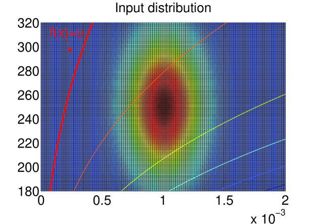
Figure 1: Input distribution and contour plot of the performance function

In the Bayesian Subset Simulation algorithm, we set an initial design of size $N_{0}=10$ which is equal to five times the dimension $d$ of the input space (In the literature, very little is known about the problem of choosing $N_{0}$, however some authors recommend to start with a sample size proportional to the dimension $d$, see  [31]). Concerning the choice of $N_{0}$, we decide to apply a greedy MAXMIN algorithm and sequentially choose the points which will maximize the minimal Euclidean distance between any two points in the initial Monte Carlo sample $\mathds{Y}_{0}$. At each stage, we choose a Monte Carlo sample of size $m=1000$. A Gaussian process with constant unknown mean and a Matérn covariance function is used as our prior information about $f$. The parameters of the Matérn covariance functions are estimated on the initial design by REML (see, e.g., [32]). In this experiment, we follow the common practice of re-estimating the parameters of the covariance function during the sequential strategy, and update the covariance function after each evaluation. The target conditional probability between successive thesholds is set to $p_{0}=0.1$. The intermediate threshold $u_{t}$ is chosen by the criterion (2.3). The proposal distribution $q_{t}$ for a Gibbs sampling is a Gaussian distribution $\mathcal{N}(0,\sigma^{2})$, where $\sigma^{2}$ is specified in Table 2. The stopping criterion for the adaptive SUR strategy is set to $\eta_{t}=10^{-6}$ (for $t=1,\ldots,T-1$) and $\eta_{T}=10^{-7}$.

Figure 2 shows the Design of Experiment (DoE) selected by the algorithm at stage $t=1,2,3$ and the last stage for one run. Table 3 lists the number of evaluations (rounded to integer) at each stage averaged over $50$ runs. We can see that an average total of evaluations $N=\sum_{i=0}^{T}N_{t}=104$ are needed for our proposed Bayesian Subset Simulation, while for Subset Simulation, the number is $1000+900\times 4=4600$.

Table 3: Average number of evaluations at each stage.

$N_{t}$	$1$	$2$	$3$	$4$	$5$
Sub-Sim	$1000$	$900$	$900$	$900$	$900$
Bayesian Sub-Sim	$14$	$17$	$17$	$18$	$28$

\psfrag{x1}{\tiny$x_{1}$}\psfrag{x2}{\tiny$x_{2}$}\psfrag{ut}{\tiny$u_{t},t=1,\ldots,T$}\includegraphics[width=195.12767pt]{T1DOE}

\psfrag{x1}{\tiny$x_{1}$}\psfrag{x2}{\tiny$x_{2}$}\psfrag{ut}{\tiny$u_{t},t=1,\ldots,T$}\includegraphics[width=195.12767pt]{T2DOE}

\psfrag{x1}{\tiny$x_{1}$}\psfrag{x2}{\tiny$x_{2}$}\psfrag{ut}{\tiny$u_{t},t=1,\ldots,T$}\includegraphics[width=195.12767pt]{T3DOE}

\psfrag{x1}{\tiny$x_{1}$}\psfrag{x2}{\tiny$x_{2}$}\psfrag{ut}{\tiny$u_{t},t=1,\ldots,T$}\includegraphics[width=195.12767pt]{TLDOE}

Figure 2: Evaluations selected by the Bayesian Subset Simulation strategy at stage $t=1,2,3$ and the final Design of Experiment (DoE).

To evaluate the statistical properties of the estimator, we consider the absolute relative bias

$$\kappa=\left|\frac{\mathsf{E}(\widehat{\alpha})-\alpha}{\alpha}\right|$$ (9)

and the coefficient of variation

$$\operatorname{cov}=\frac{\delta(\widehat{\alpha})}{\alpha},$$ (10)

where $\mathsf{E}(\widehat{\alpha})$ is the average mean and $\delta(\widehat{\alpha})$ is the standard deviation of the estimator $\widehat{\alpha}$.

Table 4 shows the results of the comparison of our proposed Bayesian Subset Sampling algorithm with the Subset Simulation algorithm in [3]. Crude Monte Carlo sampling is used as the reference probability of failure. For the fairness of the comparison, we set the same intermediate probability $p_{0}=0.1$, and sample size $m=1000$ in both methods. Fifty independent runs are performed to evaluate the average of both methods. For Bayesian Subset Simulation method, as $N$ is different for each run, we show the minimal and maximal of $N$ from $50$ runs.

Table 4: Compare with Monte Carlo approach and Subset Simulation

Method	$m$	$N$	$\widehat{\alpha}~{}(10^{-5})$	$\delta(\widehat{\alpha})~{}(10^{-5})$	$\kappa$	$\operatorname{cov}$
MCS	$10^{8}$	$10^{8}$	$3.8500$	$0.062$	$0$	$1.6\%$
Sub-Sim	$1000$	$4600$	$3.9078$	$2.470$	$1.5\%$	$63.2\%$
Bayesian Sub-Sim	$1000$	$[94,109]$	$3.7020$	$0.618$	$4.4\%$	$16.7\%$

missingum@section Conclusion

In this paper, we propose a new algorithm called Bayesian Subset Simulation for estimating small probabilities of failure in a context of very expensive simulations. This algorithm combines the main ideas of the Subset Simulation algorithm and the SUR strategies developed in our recent work [2].

Our preliminary results show that the number of evaluations is dramatically decreased compared to the original Subset Simulation algorithm, while keeping a small bias and coefficient of variation.

Our future work will try to improve further the properties of our algorithm regarding the bias and the variance of the estimator. We shall also test and validate the approach on more challenging examples.

References

- [1] E. Vazquez and J. Bect. A sequential Bayesian algorithm to estimate a probability of failure. In Proceedings of the 15th IFAC Symposium on System Identification, SYSID 2009 15th IFAC Symposium on System Identification, SYSID 2009, Saint-Malo France, 2009.
- [2] J. Bect, D. Ginsbourger, L. Li, V. Picheny, and E. Vazquez. Sequential design of computer experiments for the estimation of a probability of failure. Statistics and Computing, pages 1–21, 2010.
- [3] S. K. Au and J. Beck. Estimation of small failure probabilities in high dimensions by subset simulation. Probab. Engrg. Mechan., 16(4):263–277, 2001.
- [4] F. Cérou, P. Del Moral, T. Furon, and A. Guyader. Sequential monte carlo for rare event estimation. Statistics and Computing, pages 1–14, 2011.
- [5] J. Sacks, W. J. Welch, T. J. Mitchell, and H. P. Wynn. Design and analysis of computer experiments. Statistical Science, 4(4):409–435, 1989.
- [6] C. Currin, T. Mitchell, M. Morris, and D. Ylvisaker. Bayesian prediction of deterministic functions, with applications to the design and analysis of computer experiments. J. Amer. Statist. Assoc., 86(416):953–963, 1991.
- [7] W. J. Welch, R. J. Buck, J. Sacks, H. P. Wynn, T. J. Mitchell, and M. D. Morris. Screening, predicting and computer experiments. Technometrics, 34:15–25, 1992.
- [8] J. Oakley and A. O’Hagan. Bayesian inference for the uncertainty distribution of computer model outputs. Biometrika, 89(4), 2002.
- [9] J.E. Oakley and A. O’Hagan. Probabilistic sensitivity analysis of complex models: a Bayesian approach. Journal of the Royal Statistical Society: Series B (Statistical Methodology), 66(3):751–769, 2004.
- [10] J. Oakley. Estimating percentiles of uncertain computer code outputs. J. Roy. Statist. Soc. Ser. C, 53(1):83–93, 2004.
- [11] M. J. Bayarri, J. O. Berger, R. Paulo, J. Sacks, J. A. Cafeo, J. Cavendish, C.-H. Lin, and J. Tu. A framework for validation of computer models. Technometrics, 49(2):138–154, 2007.
- [12] J. Mockus, V. Tiesis, and A. Zilinskas. The application of Bayesian methods for seeking the extremum. In L. Dixon and Eds G. Szego, editors, Towards Global Optimization, volume 2, pages 117–129. Elsevier, 1978.
- [13] J. Mockus. Bayesian Approach to Global Optimization. Theory and Applications. Kluwer Academic Publisher, Dordrecht, 1989.
- [14] D. R. Jones, M. Schonlau, and J. William. Efficient global optimization of expensive black-box functions. Journal of Global Optimization, 13(4):455–492, 1998.
- [15] J. Villemonteix. Optimisation de fonctions coûteuses. PhD thesis, Université Paris-Sud XI, Faculté des Sciences d’Orsay, 2008.
- [16] J. Villemonteix, E. Vazquez, and E. Walter. An informational approach to the global optimization of expensive-to-evaluate functions. Journal of Global Optimization, 44(4):509–534, 2009.
- [17] D. Ginsbourger. Métamodèles multiples pour l’approximation et l’optimisation de fonctions numériques multivariables. PhD thesis, Ecole nationale supérieure des Mines de Saint-Etienne, 2009.
- [18] V. Dubourg, B. Sudret, and J.-M. Bourinet. Reliability-based design optimization using kriging surrogates and subset simulation. Structural Multisciplinary Optimization, 44(5):673–690, 2011.
- [19] V. Dubourg. Adaptive surrogate models for reliability analysis and reliability-based design optimization. PhD thesis, Université Blaise Pascal – Clermont II, 2011.
- [20] Pierre Del Moral, Arnaud Doucet, and Ajay Jasra. Sequential monte carlo samplers. Journal of the Royal Statistical Society: Series B (Statistical Methodology), 68(3):411–436, 2006.
- [21] R. Douc and É. Moulines. Limit theorems for weighted samples with applications to sequential monte carlo methods. The Annals of Statistics, 36(5):2344–2376, 2008.
- [22] Vincent Dubourg, François Deheeger, and Bruno Sudret. Metamodel-based importance sampling for structural reliability analysis. Preprint submitted to Probabilistic Engineering Mechanics, 2011.
- [23] Vincent Dubourg, François Deheeger, and Bruno Sudret. Metamodel-based importance sampling for the simulation of rare events. In 11th International Conference on Applications of Statistics and Probability in Civil Engineering (ICASP 11), 2011.
- [24] Christian P. Robert and G. Casella. Monte Carlo statistical methods, 2nd edition. Springer Verlag, 2004.
- [25] T. J. Santner, B. J. Williams, and W. Notz. The Design and Analysis of Computer Experiments. Springer Verlag, 2003.
- [26] J. D. Hol, T. B. Schon, and F. Gustafsson. On resampling algorithms for particle filters. In IEEE Workshop on Nonlinear Statistical Signal Processing Workshop, pages 79–82, 2006.
- [27] Randal Douc and Olivier Cappé. Comparison of resampling schemes for particle filtering. In Proceedings of the 4th International Symposium on Image and Signal Processing and Analysis (ISPA), pages 64–69, 2005.
- [28] M. Bolic, Petar M. Djurić, and S. Hong. New resampling algorithms for particle filters. In IEEE International Conference on Acoustics, Speech, and Signal Processing, 2003. Proceedings.(ICASSP’03), volume 2, pages 589–592, 2003.
- [29] N. Gayton, J.M. Bourinet, and M. Lemaire. Cq2rs: a new statistical approach to the response surface method for reliability analysis. Structural Safety, 25(1):99–121, 2003.
- [30] M.R. Rajashekhar and B.R. Ellingwood. A new look at the response surface approach for reliability analysis. Structural Safety, 12(3):205–220, 1993.
- [31] Jason L. Loeppky, Jerome Sacks, and William J. Welch. Choosing the sample size of a computer experiment: A practical guide. Technometrics, 51(4):366–376, 2009.
- [32] M. L. Stein. Interpolation of Spatial Data: Some Theory for Kriging. Springer, New York, 1999.