Condensed Matter Theory of Dipolar Quantum Gases
1 Introduction.
The realization of Bose Einstein condensates (BEC) and quantum degenerate Fermi gases with cold atoms have been highlights of quantum physics during the last decade. Cold atoms in the tens of nanokelvin range are routinely obtained via combined laser- and evaporative-cooling techniques 1. For high-enough densities ( ), the atomic de Broglie wavelength becomes larger than the typical interparticle distance and thus quantum statistics governs the many-body dynamics of these systems. Characteristic features of the physics of cold atomic gases are the microscopic knowledge of the many-body Hamiltonians which are realized in the experiments and the possibility of controlling and tuning system parameters via external fields. External field control of contact inter-particle interactions can be achieved, for example, by varying the scattering length via Feshbach resonances 2, while trapping of ultracold gases is obtained with magnetic, electric and optical fields 3. In particular, optical lattices, which are artificial crystals made of light obtained via the interference of optical laser beams, can realize perfect arrays of hundreds of thousands of microtraps 4, 5, allowing for the confinement of quantum gases to one-dimensional (1D), 2D and 3D geometries and even the manipulation of individual particles 6, 7. This control over interactions and confinement is the key for the experimental realization of fundamental quantum phases and phase transitions as illustrated by the BEC-BCS crossover in atomic Fermi gases 8, and the Berezinskii-Kosterlitz-Thouless transition 9 for cold bosonic atoms confined to 2D.
Breakthroughs in the experimental realization of BEC and degenerate Fermi gases of atoms with a comparatively large magnetic dipole moment, such as 10, 11, 12, 13, 14, 15, 16, 17 and 164Dy atoms 18, 19 (dipole moment and 10, respectively, with Bohr’s magneton), and the recent astounding progress in experiments with ultracold polar molecules 20, 21, 22, 23, 24, 25, 26, 27, 28, 29, 30, 31 have now stimulated great interest in the properties of low temperature systems with dominant dipolar interactions (see reviews Refs. 32, 33, 34, 35, 36 for discussions of various aspects of the problem). The latter have a long-range and anisotropic character, and their relative strength compared to, e.g., short-range interactions can be often controlled by tuning external fields, or else by adjusting the strength and geometry of confining trapping potentials. For example, in experiments with polarized atoms, magnetic dipolar interactions can be made to overcome short-range interactions by tuning the effective -wave scattering length to zero using Feshbach resonances 10, 11, 12, 13. This has already led to the observation of fundamental phenomena at the mean-field level, such as, the anisotropic deformation during expansion and the directional stability 37, 18 of dipolar BECs. Heteronuclear polar molecules in a low vibrational and rotational state, on the other hand, can have large permanent dipole moments along the internuclear axis with strength ranging between one tenth and ten Debye (1Debye C m). In the presence of an external electric field (with a typical value of V/cm) mixing rotational excitations, the molecules can be oriented in the laboratory frame and the induced dipole moment can approach its asymptotic value, corresponding to the permanent dipole moment. This effect can be used to tune the strength of the dipole-dipole interaction 35. Additional microwave fields allow for advanced tailoring of the interactions between the molecules, where even the shape of interaction potentials can be tuned with external fields, in addition to the strength. This tunability of interactions forms the basis for the realization of novel quantum phenomena in these systems, in the strongly interacting limit.
As a result of this progress, in recent years dipolar gases have become the subject of intensive theoretical efforts, and there is now an extensive body of literature predicting novel properties for these systems32, 33, 34, 35, 36. It is the purpose of this review to provide a summary of these recent theoretical studies with a focus on the many-body quantum properties, to demonstrate the connections and differences between dipolar gaseous systems and traditional condensed-matter systems, and to stress the inherent interdisciplinary nature of these studies. This work covers spatially homogeneous as well as trapped systems, and includes the analysis of the properties of dipolar gases in both the mean-field (dipolar Bose-Einstein condensates and superfluid BCS pairing transition) and in the strongly correlated (dipolar gases in optical lattices and low-dimensional geometries) regimes.
We tried our best to include all relevant works of this exciting, ever expanding field. We apologize in advance if some papers (hopefully, not many) are not appearing below.
2 The dipole-dipole interaction
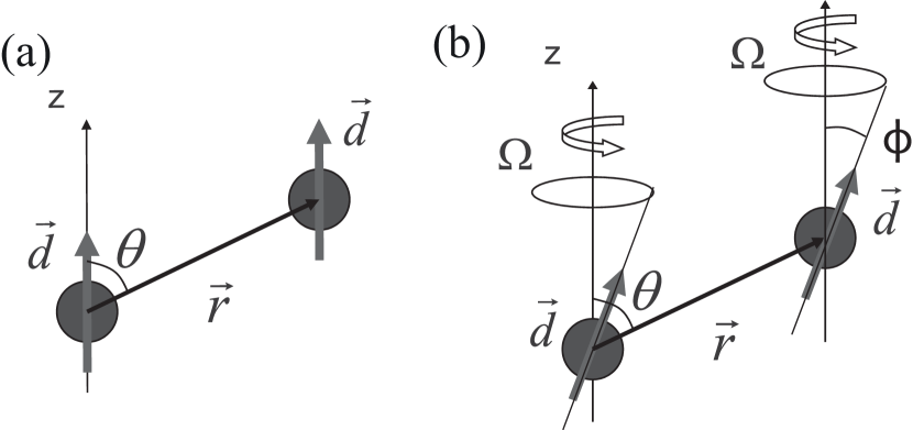
For polarized dipolar particles, interparticle interactions include both a short-range Van der Waals (vdW) part and a long-range dipole-dipole one. The latter is dominant at large interparticle separations and assuming a polarization along the -axis as in Fig. 1(a) the interparticle interaction reads
| (1) |
Here is the electric dipole moment (for magnetic dipoles should be replaced with , with the magnetic dipole moment), is the vector connecting two dipolar particles, and is the angle between and the dipole orientation (the -axis). The potential is both long-range and anisotropic, that is, partially repulsive and partially attractive. As discussed in the sections below, these features have important consequences for the scattering properties in the ultracold gas, for the stability of the system as well as for a variety of its properties.
2.1 Scattering of two dipoles
The long-range character () of the dipole-dipole interaction results in all partial waves contributing to the scattering at low energies, and not only, e.g., the -wave, as is often the case for short-range interactions. In fact, for dipole-dipole interactions the phase shift in a scattering channel with angular momentum behaves as for and small (see, e.g., Refs. 38 and 39).
The effect of the anisotropy of the interaction is instead that the angular momentum is not conserved during scattering: for bosons and fermions the dipole-dipole interaction mixes all even and odd angular momenta scattering channels, respectively. Due to the coupling between the various scattering channels, the potential then generates a short-range contribution to the total effective potential in the -wave channel (). This has the general effect to reduce the strength of the short-range part of the interaction.
Thus, for two bosonic dipolar particles (even angular momenta) the scattering at low energies is determined by both the long-range and the short-range parts of the interaction. This is in contrast to the low energy scattering of two fermionic dipoles (odd angular momenta), which is universal in the sense that it is determined only by the long-range dipolar part of the interaction, and is insensitive to the short-range details.
For a dilute weakly interacting gas the above results allow a parametrization of the realistic interparticle interaction between two particles of mass in terms of the following pseudopotential 40-41 (see also Refs. 42 and 43)
| (2) |
with
| (3) |
parametrizing the short-range part of the interaction. We note that the long-range part of the
pseudopotential is identical to the long-range part of the original potential
and the scattering length controlling the short-range part depends on the dipole moment.
This dependence is important 44 when one changes the dipole moment,
using external, e.g. electric, fields, as explained below.
The strength of the dipole-dipole interaction can be characterized by the quantity
which has the dimension of length and can be considered as a characteristic range of the dipole-dipole interaction, or dipolar length. This length determines the low energy limit of the scattering amplitudes, and, in this sense, is analogous to the scattering length for the dipole-dipole interaction. For chromium atoms with a comparatively large magnetic moment of (equivalent dipole moment Debye) we have nm. For most polar molecules the electric dipole moment ranges in between and Debye, while ranges from to nm. For example, the dipole moment of fermionic ammonia molecules is Debye with nm, while for it increases to Debye and nm. This latter value of the effective scattering length is an order of magnitude larger than, for example, the one for the intercomponent interaction in the widely discussed case of a two-species fermionic gas of , where nm. Thus, the strength of the dipole-dipole interaction between polar molecules can be not only comparable with but even much larger than the strength of the short-range interatomic interaction.
2.2 Tunability of the dipole-dipole interaction
One spectacular feature of the dipole-dipole interaction is its tunability. In Sect. 2.2.1 we first review methods for tuning the strength and sign of dipolar interactions with an eye to cold atoms, and then in Sect. 2.2.2 we discuss tunability for the specific case of polar molecules, where both the strength as well as the shape of interactions can be engineered.
2.2.1 Tunability of interactions in cold atoms
In Ref. 45 a technique has been developed to tune the strength as well as the sign of dipolar interactions in atomic systems with a finite permanent magnetic dipole moment. This technique uses a combination of a static (e.g., magnetic) field along the -axis and a fast rotating field in the perpendicular -plane such that the resulting time dependent dipole moment is [see Fig. 1(b)]
Here is the rotating frequency of the field and the angle , is determined by the ratio of the amplitudes of the static and rotating fields. The above expression implies that the dipoles follow the time-dependent external field adiabatically. This in turn sets an upper limit on the values of the rotating frequency , which should be (much) smaller than the level splitting in the field. However, if the frequency is much larger that the typical frequencies of the particle motion, over the period the particles feel an average interaction
The latter differs from the interaction for aligned dipoles, Eq. (1), by a factor , which can be changed continuously from to by varying the angle . Thus this method allows to ”reverse” the sign of the dipole-dipole interaction and even cancel it completely for , similar to NMR techniques 46. We note that an analogous technique can be also applied for the electric dipole moments of, e.g., polar molecules. We will review applications of this method below.
2.2.2 Effective Hamiltonians for polar molecules
In the following we will be often interested in manipulating interactions for
polar molecules in the strongly interacting regime. In particular, we
will aim at modifying not only the strength but also the shape of
interaction potentials, as a basis to investigate new condensed matter
phenomena. This usually entails a combination of the following two steps: (i)
manipulating the internal (electronic, vibrational, rotational, …) structure
of the molecules, and thus their mutual interactions, using external static
(DC) electric and microwave (AC) fields, and (ii) confining molecules to a
lower-dimensional geometry, using, e.g., optical potentials, as exemplified in
Fig. 2. Under appropriate conditions, the resulting effective
interactions can be made purely repulsive at large distances (e.g.,
at characteristic distances of 10nm or more), as in the 2D example of
Fig. 3(a). On one hand, this has the effect to suppress
possible inelastic collisions and chemical reactions occurring at short-range
(i.e., at characteristic distances of nm), and on the other
hand it allows to study interesting condensed matter phenomena originating
from the often-unusual form of the two-body (or many-body-) interaction
potentials. In the next few subsections we review techniques for the
engineering of the interaction potentials which will be used in the many-body
context in Sect. 6 below.
Our starting point is the Hamiltonian for a gas of cold heteronuclear molecules prepared in their electronic and vibrational ground-state,
| (4) |
Here the first term in the single particle Hamiltonian corresponds to the kinetic energy of the molecules, while represents a trapping potential, as provided, for example, by an optical lattice, or an electric or magnetic trap. The term describes the internal low energy excitations of the molecule, which for a molecule with a closed electronic shell (e.g. SrO, RbCs or LiCs) correspond to the rotational degree of freedom of the molecular axis. This term is well described by a rigid rotor with the rotational constant (in the few to tens of GHz regime) and the dimensionless angular momentum. The rotational eigenstates for a quantization axis , and with eigenenergies can be coupled by a static (DC) or microwave (AC) field via the electric dipole moment , which is typically of the order of a few Debye.
In the absence of electric fields, the molecules prepared in a ground
rotational state have no net dipole moment, and interact via a
van-der-Waals attraction , reminiscent of
the interactions of cold alkali metal atoms in the electronic ground-states.
Electric fields admix excited rotational states and induce static or
oscillating dipoles, which interact via strong dipole-dipole interactions
with the characteristic dependence given in Eq. (1).
For example, a static DC field couples the spherically symmetric rotational
ground state of the molecule to excited rotational states with different
parity, thus creating a non-zero average dipole moment. The field strength
therefore determines the degree of polarization and the magnitude of the
dipole moment. As a result, the effective dipole-dipole interaction may be
tuned by the competition between an orienting, e.g., DC electric field and the
quantum (or thermal) rotation of the molecule. This method effectively works
for the values of the field up to the saturation limit, at which the molecule
is completely polarized (typically V/cm).
The many body dynamics of cold polar molecules is thus governed by an interplay between dressing and manipulating the rotational states with DC and AC fields, and strong dipole-dipole interactions. In condensed matter physics one is often interested in effective theories for the low-energy dynamics of the many-body system, after the high-energy degrees of freedom have been traced out. The connection between the full molecular -particle Hamiltonian (4) including rotational excitations and dressing fields, and an effective low-energy theory can be made using the following Born-Oppenheimer approximation: The diagonalization of the Hamiltonian for frozen spatial positions of the molecules yields a set of energy eigenvalues , which can be interpreted as the effective interaction potential in the single-channel many-body Hamiltonian
| (5) |
The term represents an effective -body interaction, which can be expanded as a sum of two-body and many-body interactions
| (6) |
where in most cases only two-body interactions are considered. The dependence
of on the
electric fields provides the basis for the engineering of the
many body interactions, as described below.
We note that the attractive part of the interaction potential can induce instabilities in a dipolar gas at the few body level as well as at the many-body level (this latter case will be discussed in Sect. 3 below). For example, for several experimentally relevant mixed alkali-metal diatomic species such as KRb, LiNa, LiK, LiRb, and LiCs 47 there exist chemically reactive channels that are energetically favorable, leading to particle recombination and two-body losses in the gas. The rate of chemical reactions can be strongly enhanced by dipole-dipole interactions which can attract molecules in a head-to-tail configuration [e.g., in Fig. 1(a)] to distances on the order of typical chemical interaction distances, nm 48, 49, 50, 51, 52, 53, 54, 55, 56. One aim of interaction engineering is to control these interactions in order to stabilize the gas against particle losses. This will enable the study of complex condensed matter phenomena in these systems.
2.2.3 Stabilization of dipolar interactions in 2D
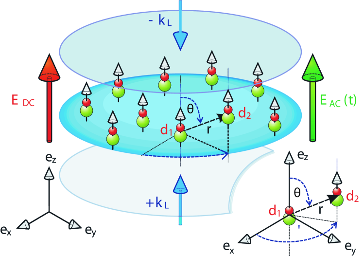
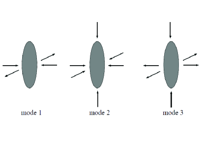
The simplest example of stabilization of dipolar interactions against inelastic collisions is sketched in Fig. 2 and consists of a system of cold polar molecules in the presence of a polarizing DC electric field oriented in the -direction, and of a strong harmonic transverse confinement with frequency and characteristic length . The latter is provided, e.g., by an optical lattice along .
Figure 3(b) shows a countour plot of the interaction potential for two dipoles in this quasi-2D geometry, where
Here represents the distance between the two molecules in cylindrical coordinates, and . The first term is the isotropic vdW potential, assuming the molecules are in their rotational ground state, with a vdW length 58, 59. The second term is the anisotropic dipolar potential, with induced dipole moment and dipolar length .
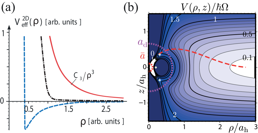
Figure 3(b) illustrates essential features of reduced dimensional collisions: for finite , the repulsive dipole-dipole interaction overcomes the attractive van-der-Waals potential in the ()-plane at distances , realizing a repulsive in-plane potential barrier (blue dark region). In addition, the harmonic potential confines the particles’s motion in the direction. The combination of the dipole-dipole interaction and of the harmonic confinement thus yields a three-dimensional potential barrier separating the long-distance, where interactions are repulsive, from the short-distance one, where interactions are attractive and inelastic processes can occur. If the collision energy is smaller than the height of the barrier at the saddle point (white circles), the particles’ motion is confined to the long-distance region, where particles scatter elastically. Particle losses are due to tunneling through the potential barrier at a rate . Within a semiclassical (instanton) approximation valid for , the tunneling rate is well approximated by the exponential form
| (7) |
The constant has been recently computed numerically by Julienne, Hanna and
Idziaszek 61 to be , while the ”attempt rate”
62 for the scattering of two isolated dipoles
reads ,
independent of particles’ statistics. Here is the momentum
for a collision with relative kinetic energy , with the DeBroglie wavelength. For
particles in a crystalline configuration (see Sect. 6.1
below), will be proportional to the frequency of phonon
oscillations around the mean particle positions , with the mean inter-particle distance. The
expression Eq. (7) shows that collisional losses may be
strongly suppressed for any molecular species for a large enough
dipole moment or strength of transverse confinement.
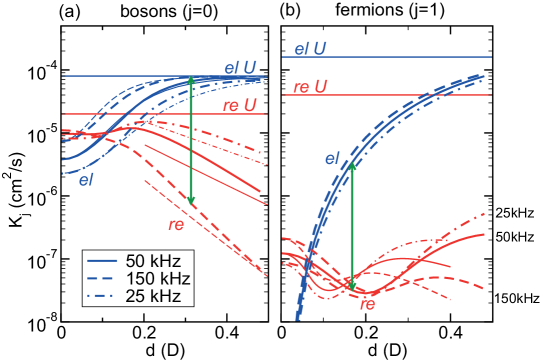
In ultracold collisions one often has the following separation of length scales: , and can be tuned by, e.g, increasing the external DC field. Figure 4(a) and (b) show numerical results for reactive and elastic collision rates of bosonic and fermionic KRb molecules, respectively, and for several strengths of transverse confinement. Here , and are on the order of hundreds of nm, tens of nm, and less than 10 nm, respectively. Because of the moderate D of KRb molecules, here and the semiclassical regime of large of Eq. (7) is not reached. Nevertheless, in stark contrast to collisions in 3D 50, the figure shows that the ratio between elastic and inelastic collision rates increases rapidly with , signaling an increased stability with increasing . For bosons, the exact numerical results (thick lines) approach rapidly the semiclassical instanton limit (thin lines) with increasing . The behavior of the inelastic rates for fermions is explained in detail in Refs. 63, 60.
Recent landmark experimental results from the JILA group with fermionic KRb molecules show a strong suppression of inelastic collisions and increase of elastic ones with , in excellent agreement with the predictions of Fig. 3. This opens the way to the study of strongly correlated phenomena in these systems.
2.2.4 Advanced interaction designing: Blue-shielding
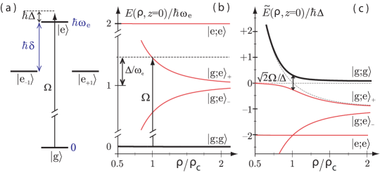
By combining DC and AC fields to dress the manifold of rotational energy levels it is possible to design effective interaction potentials with (essentially) any shape as a function of distance. For example, the addition of a single linearly-polarized AC field to the configuration of Sect. 2.2.3 leads to the realization of the 2D “step-like” potential of Fig. 3(a) (black dashed-dotted line), where the character of the repulsive potential varies considerably in a small region of space. The derivation of this effective 2D interaction is sketched in Fig. 5(a-c) 64, 57. The (weak) DC-field splits the first-excited rotational ()-manifold of each molecule by an amount , while a linearly polarized AC-field with Rabi frequency is blue-detuned from the ()-transition by , see Fig. 5(a). Because of and the choice of polarization, for distances the relevant single-particle states for the two-body interaction reduce to the states and of each molecule. Figure 5(b) shows that the dipole-dipole interaction splits the excited state manifold of the two-body rotational spectrum, making the detuning position-dependent. As a consequence, the combined energies of the bare groundstate of the two-particle spectrum and of a microwave photon become degenerate with the energy of a (symmetric) excited state at a characteristic resonant (Condon) point , which is represented by an arrow in Fig. 5(b). At this Condon point, an avoided crossing occurs in a field-dressed picture, and the new (dressed) groundstate potential inherits the character of the bare ground and excited potentials for distances and , respectively. Fig. 5(d) shows that the dressed groundstate potential (which has the largest energy) is almost flat for and it is strongly repulsive as for , which corresponds to the realization of the step-like potential of Fig. 3(a). We remark that, due to the choice of polarization, this strong repulsion is present only in the plane , while for the groundstate potential can become attractive. The optical confinement along of Sect. 2.2.3 is therefore necessary to ensure the stability of the system.
The interactions in the presence of a single AC field are described in detail in Ref. 57, where it is shown that in the absence of external confinement this case is analogous to the (3D) optical blue-shielding developed in the context of ultracold collisions of neutral atoms 65, 66, 67, however with the advantage of the long lifetime of the excited rotational states of the molecules, as opposed to the electronic states of cold atoms. The strong inelastic losses observed in 3D collisions with cold atoms 65, 66, 67 can be avoided via a judicious choice of the field’s polarization, eventually combined with a tight confinement to ensure a 2D geometry (as e.g. in Fig. 2 above). For example, in Ref. 68 it is shown that in the presence of a DC field and of a circularly polarized AC field the attractive time-averaged interaction due to the rotating (AC-induced) dipole moments of the molecules allows for the cancelation of the total dipole-dipole interaction. The residual interactions remaining after this cancelation are purely repulsive 3D interactions with a characteristic van-der-Waals behavior . This 3D repulsion provides for a shielding of the inner part of the interaction potential and thus it will strongly suppress inelastic collisions in experiments.
Recent works 69, 70 have considered the microwave
spectra of alkali-metal dimers including hyperfine interactions. It is an
important open question to determine the effects that the presence of internal
states such as, e.g. hyperfine states, have on the broad class of shielding
techniques described above.
3 Weakly interacting dipolar Bose gas
3.1 BEC in a spatially homogeneous gas.
Let us discuss now the influence of the dipole-dipole interaction on the properties of a homogeneous single-component dipolar Bose gas 111This and the next Sections are substantially revised and updated version of the corresponding part of Ref. 32. This can be most conveniently done in the language of second quantization. For this purpose we introduce particle creation and annihilation field operators and satisfying standard bosonic commutation relation
The corresponding second quantized Hamiltonian of the system then reads
| (8) | |||||
where is the mass of the particles, is the interparticle interaction, and the chemical potential fixes the average density of the gas. We consider the case when the system is away from any ”shape” resonances 38,39,71 and, therefore, replace the original interparticle interaction with the pseudopotential (2). Assuming that the system is dilute, , we can write the Hamiltonian as
| (9) | |||||
where is given by Eq. (1) and [as compared to Eq. (3), we omit the dependence of the scattering length on the dipole moment ]. Note that the scattering length has to be positive, , to avoid an absolute instability due to local collapses 72.
As we will see below, an important parameter that determines the properties of the system described by the Hamiltonian (9) is
| (10) |
It measures the strength of the dipole-dipole interaction relative to the short-range repulsion. In the case , the short-range part of the interparticle interaction is dominant while the dipole-dipole interaction results in only small corrections. For a positive scattering length , the system is stable and exhibits BEC at low temperatures. This case corresponds to earlier experiments 10, 13 with Cr BEC ( 13). It was found that the corrections due to magnetic dipole-dipole interaction between 52Cr atoms are of the order of .
For the opposite case , the anisotropic dipole-dipole interaction plays the dominant role resulting in instability of a spatially homogeneous system 73,74, 75. This instability can be seen in the dispersion relation between the energy and the momentum of excitations in the Bose-condensed gas, which can be easily obtained within the standard Bogoliubov approach:
Here is the angle between the excitation momentum and the direction of dipoles, and is the Fourier transform of . For , the excitation energies at small and close to become imaginary signalling the instability (collapse). This instability of a spatially homogeneous dipolar Bose gas with dominant dipole-dipole interaction is a result of a partially attractive nature of the dipole-dipole interaction.
3.2 BEC in a trapped gas.
The above consideration shows that the behavior of a spatially homogeneous Bose gas with a strong dipole-dipole interaction is similar to that of a Bose gas with an attractive short-range interaction characterized by a negative scattering length . In the latter case, however, the collapse of the gas can be prevented by confining the gas in a trap provided the number of particles in the gas is smaller than some critical value , (see, e.g., 72). This is due to the finite energy difference between the ground and the first excited states in a confined gas. For a small number of particle this creates an effective energy barrier preventing the collapse and, therefore, results in a metastable condensate. The same arguments are also applicable to a dipolar BEC in a trap, see Refs. 15 and 16, with one very important difference: The sign and the value of the dipole-dipole interaction energy in a trapped dipolar BEC depends on by the trapping geometry and, therefore, the stability diagram contains the trap anisotropy as a crucial parameter.
3.2.1 Ground state.
The Hamiltonian for a trapped dipolar Bose gas reads
where
| (13) |
is the trapping potential and we again use the pseudopotential (2) for the short-range part of the interparticle interaction assuming that the system is away from ”shape” resonances. For the trapping potential we consider the experimentally most common case of an axially symmetric harmonic trap characterized by the axial and radial trap frequencies. The aspect ratio of the trap is defined through the ratio of the frequencies: , where and are the axial and radial sizes of the ground state wave function in the harmonic oscillator potential (13), respectively. For one has a pancake-form (oblate) trap, while the opposite case corresponds to a cigar-form (prolate) trap. Taking into account the anisotropy of the dipole-dipole interaction, one can easily see that the aspect ratio should play a very important role in the behavior of the system.
The standard mean-field approximation corresponds to taking the many-body wave function in the form of a product of single-particle wave functions:
| (14) |
The condensate is then described by the condensate wave function normalized to the total number of particles, , and governed by the time-dependent Gross-Pitaevskii (GP) equation
| (15) | |||||
The validity of this approach was tested in Refs. 44 and 41 by using many-body diffusion Monte-Carlo calculations with the conclusion that a GP equation with the pseudopotential (2) provides a correct description of the gas in the dilute limit . Note that, being the product of single-particle wave functions, the many-body wave function (14) does not take into account interparticle correlations at short distances due to their interaction, which takes place at interparticle distances . This change of the wave function is taken into account in Eq. (15) by the contact part of the pseudopotential (2) [the fourth term in the right-hand-side in Eq. (15)] but ignored in the last term of Eq. (15) because the main contribution to the integral comes from large interparticle distances (of order the spatial size of the condensate).
Let us first consider stationary solutions of Eq. (15), for which and obeys the stationary GP equation
| (16) |
where . Numerical analysis of Eqs. (15) and (16) was performed in Refs. 40,73, 74,76-77 on the basis of numerical solutions of the non-linear Schrödinger equation (16) together with variational considerations with the Gaussian ansatz for the condensate wave function. In Refs. 44 and 41 the problem was treated using diffusive Monte-Carlo calculations, while the authors of Ref. 78 apply the Thomas-Fermi approximation that neglects the kinetic energy and allows to obtain analytical results.
We begin the discussion of the results with the case of a dominant dipole-dipole interaction, , such that the third term in the left-hand-side of Eq. (16) can be neglected. This case demonstrates already all important features of the behavior of dipolar condensates. The general case will be briefly discussed at the end of this section.
Let us introduce the mean-field dipole-dipole interaction energy per particle
| (17) |
which together with the trap frequencies and are important energy scales of the problem. One can easily see that the value of the chemical potential and the behavior of the dipolar condensate are determined by the aspect ratio of the trap , the quantity , and the parameter . Notice also that the anisotropy of the dipole-dipole interaction results in squeezing the cloud in the radial direction and stretches it in the axial one (along the direction of dipoles) in order to low the interaction energy. For this reason the aspect ratio of the cloud is always larger than the aspect ratio of the trap. Here and are the axial and the radial sizes of the cloud, respectively.
We now summarize the results of the stability analysis of the dipolar condensate with (Eq. (16) with ) 74,76,79 (see also Ref. 77 for the stability analysis in a general harmonic trap). The mean-field dipole-dipole interaction is always attractive, , for a cigar shaped trap causing instability (collapse) of the gas if the particle number exceeds a critical value . This critical value depends only on the trap aspect ratio . It was found that the shape of the cloud with close to is approximately Gaussian with the aspect ratio for a spherical trap (), and for an elongated trap with .
For a pancake shaped trap with , the situation is more subtle. In this case there exists a critical trap aspect ratio , which splits the pancake shaped traps into soft pancake traps () and hard pancake traps (). For soft pancake traps one has again a critical number of particles such that the condensates with are unstable. For close to and , the aspect ratio of the cloud approaches the aspect ratio of the trap, . Note that in this case the collapse occurs even in a pancake shaped cloud with positive mean dipole-dipole interaction due to the behavior of the lowest quadrupole and monopole excitations (see Section 3.2.2).
For hard pancake traps, it was argued in Refs. 74 and 76 that the dipolar condensate is stable for any because the dipole-dipole interaction energy is always positive. On the other hand, by using more advanced numerical analysis and larger set of possible trial condensate wave functions, the authors of Ref. 79 found that the dipolar condensate in a hard pancake trap is also unstable for sufficiently large number of particles. Similar conclusions were drawn in Ref. 77. It was found that the critical values of the parameter for the instability to occur are orders of magnitude larger than in soft pancake and cigar shaped traps. In addition, the regions in parameter space were discovered where the maximum density of the condensate is not in the center of the cloud such that the condensate has a biconcave shape. (Analogous behavior of the condensate in a general three-dimensional harmonic trap were found in Ref. 77, see also 80 and 81.) These regions exist also in the presence of a small contact interaction with , but their exact position and size depend on . It is important to mention that condensates with normal and biconcave shapes behave differently when the instability boundary is crossed. The condensate with a normal shape develops a modulation of the condensate density in the radial direction, so-called ”radial roton” instability similar to the roton instability for the infinite-pancake trap () 82, see Section 3.2.3. On the other hand, it is the density modulations in the angular coordinate that lead to the collapse of biconcave condensates - a kind of “angular roton” instability in the trap. In the latter case one has spontaneously broken cylindrical symmetry.
The behavior of the trapped dipolar condensate can be simply captured by means of a Gaussian variational ansatz for the condensate wave function :
| (18) |
where the equilibrium radial size and the cloud aspect ratio can be found by minimizing the energy. Note that in order to describe biconcave shaped condensates, one has to consider (see Ref. 79) a linear combination of two wave functions: the first one is a Gaussian (18) and the second one is the same Gaussian multiplied by , where is the Hermite polynomial of the second order.
For large values of the parameters , where or , are large (but still ), one can use the Thomas-Fermi approximation to find the chemical potential and the shape of the cloud 78. This case corresponds to the small the kinetic energy, as compared to other energies, and, therefore, we can neglect the corresponding term with derivatives in Eq. (16). The GP equation then becomes
| (19) | |||
The solution of this equation reads
with the chemical potential
where is the density of the condensate in the center of the trap and
| (20) |
The energy of the condensate is
| (21) |
and the radii of the condensate in the radial and axial directions and are
| (22) | |||||
| (23) |
and the corresponding aspect ratio of the cloud can be found from the equation
| (24) |
Note, that the above equation coincides with the equation on the aspect ratio for the Gaussian variational ansatz (18) when the kinetic energy contribution is neglected, as shown in Ref. 73. It was also found that the Thomas-Fermi approximation agrees well with numerical results when used to analyze the stability of the condensate. However, the critical number of particles cannot be found in the Thomas-Fermi approximation because both terms in the expression (21) for the energy have the same dependence on the number of particles after taking into account the expressions (22) and (23) for and .
Let us now briefly discuss the stability of a dipolar condensate in the general case with . It is obvious that for an attractive short-range interaction with the condensate can only be (meta)stable for a small number of particles. For a repulsive short-range interaction with and weak dipole-dipole interaction , the condensate is always stable. For the dipolar condensate can be only metastable for number of particles smaller than a critical value, , which depends on and the trap aspect ratio . This means that the (metastable)condensate solution provides only a local minimum of the energy, while the global minimum presumably corresponds to a collapsed state with or, for , a kind of density modulated state.
3.2.2 Collective excitations and instability.
We have already mentioned that collective excitations play an important role in the stability analysis of a dipolar condensate. They also determine the dynamics of the gas and, therefore, are of experimental interest.
For a trapped dipolar condensate, the analysis of excitations is usually performed on the basis of the Bogoliubov-de Gennes equations which can be obtained by linearizing the time-dependent GP equation (15) around the stationary solution . This can be achieved by writing a solution of Eq. (15) in the form
where the second term describes small () oscillations of the condensate around with (complex) amplitudes and . To the first order in the linearization of Eq. (15) gives the Bogoliubov-de Gennes equations
| (25) | |||||
| (26) |
where is given by Eq. (2). The solution of these linear equations provides the eigenfunctions (,) with the amplitudes and obeying the normalization condition
and the corresponding eigenfrequencies of the collective modes. The Bogoliubov-de Gennes equations (25) and (26) can also be obtained by diagonalizing the Hamiltonian (3.2.1) in the Bogoliubov approximation, which corresponds to splitting the field operator into its mean-field value and the fluctuating quantum part expressed in terms of annihilation and creation operators and of bosonic quasiparticles (quanta of excitations):
The normalization condition for the amplitudes and ensures the bosonic nature of the excitations: The operators and obey the canonical Bose commutation relations.
Nonlocality of the dipole-dipole interaction results in an integrodifferential character of the Bogoliubov-de Gennes equations (25) and (26), making it hard to analyze them both analytically and numerically. A simpler way is to study the spectrum of small perturbations around the ground state solution of the time-dependent GP equation (15) (see Ref. 83 for this approach to atomic condensates). Using this approach in combination with the Gaussian variational ansatz 73, 84 or the Thomas-Fermi approximation 85, it is possible to obtain analytic results for several low energy excitation modes.
As an illustration, let us consider a Gaussian variational wave function
The variational parameters here are the complex amplitude , the widths , the coordinates of the center of the cloud , and the quantities and related to the slope and the curvature, respectively. The normalization of the wave function to the total number of particles provides the constraint
| (28) |
To find the equations governing the variational parameters, we notice that the time-dependent GP equation (15) are equivalent to the Euler-Lagrange equations for the action
| (29) |
with the Lagrangian
We therefore can obtain an effective Lagrangian that depends on the variational parameters by inserting Eq. (3.2.2) into Eq. (3.2.2) and integrating over space coordinates. We obtain
| (30) | |||||
where is the phase of [the modulus of was excluded by using Eq. (28)] and we set and for simplicity (this corresponds to ignoring the so-called sloshing motion of the condensate). The standard Euler-Lagrange variational procedure
with (, ) provides equations of motion for the parameters , and :
and
| (31) |
The above equation describes the motion of a particle with a unit mass in the potential
| (32) | |||||
Therefore, the frequencies of small amplitude oscillations around the stationary solution can be read from the second derivatives of the potential at its minimum. In this way one can obtain the frequencies for the first three compressional excitation modes. In Refs. 73 and 84, these frequencies and the corresponding shapes of the cloud oscillations were found for a cylindrical symmetric trap, , , see Fig. 6.
In the considered cylindrical geometry with dipoles are oriented along the -axis, the projection of the angular momentum on the -axis is a good quantum number that can characterize the mode: One has for modes and and for mode . The modes and as often called breathing and quadrupole modes, respectively, and we will follow this convention here. (In the Thomas-Fermi approximation, one can find analytical expressions for these modes, see Ref. 85.) Important is that with increasing the strength of the dipole-dipole interaction, the quadrupole mode 3 demonstrates the tendency towards instability, and becomes unstable when reaches some critical value. This character of instability via softening of the mode 2 is similar to that in a Bose gas with a short-range attractive interaction ().
The situation for a dipolar gas with dominant dipole interactions is more complicated 79,84, 86. It was found (see Ref. 84) that the instability of collective modes of a dipolar BEC reminds that of a gas with an attractive short-range interaction only if the trap aspect ratio is larger than the critical one, (numerically was found ): The lowest frequency ”breathing” mode 2 becomes unstable when the parameter . The variational approach discussed above provides the scaling behavior of its frequency near the critical point (see Ref. 84): , with , which is very close to the experimental value for Chromium BEC 15.
For intermediate values of above (), the mode which drives the instability (the lowest frequency mode) is a superposition of breathing and quadrupole modes with the exponent still close to . The mode has the breathing symmetry (mode 2) for far below , while it changes and becomes quadrupole-like (mode 3) as approaches the critical value .
For close to () the lowest frequency is the quadrupole mode 3. The frequency of this mode tends to zero as approaches the critical value, , with the exponent if is not too close to . When approaches , one has , and . Finally, when , the frequency of the lowest frequency quadrupole mode can be zero only for 86. (Note that this result cannot be reproduced within the Gaussian variational ansatz, which in general does not provide reliable results close to the instability, see Ref. 84.)
Collective modes for the case were analyzed in Ref. 79 on the basis of the Bogoliubov-de Gennes equations (25) and (26). The two possible type of solutions for the stable condensate were already mentioned above: A pancake (normal) shaped condensate (the maximum condensate density is in the center of the trap), and a biconcave shaped condensate (the maximum condensate density is at some distance from the center of the trap). It was found that in the case of a pancake condensate, the mode which drives the instability has zero projection of angular momentum on the -axis, , and consists of a radial nodal pattern. The number of the nodal surfaces increases with decreasing (flattening of the condensate). This “radial roton” mode in a confined gas can be viewed as an analog of the roton mode in an infinite-pancake trap from Ref. 82, see below. In a biconcave condensate near the instability, the lowest frequency mode has non-zero projection of the angular momentum on the -axis, . This mode is an “angular roton” in the trap: For a biconcave-shaped condensate, the maximum density is along the ring, and an angular roton corresponds to density modulation along this ring. The instability in this case corresponds to the collapse of the condensate due to buckling of the density in the angular coordinate, and, therefore, breaks the cylindrical symmetry spontaneously (see Ref. 79 for more details).
3.2.3 Roton instability of a quasi 2D dipolar condensate.
Let us now discuss the effects of the long-range and anisotropic character of dipole-dipole forces in the physically simpler case of an infinite pancake shaped trap, with the dipoles perpendicular to the trap plane 82. It was found that a condensate with a large density can be dynamically stable only when a sufficiently strong short-range repulsive interaction is present. Otherwise, excitations with the certain in-plane momenta become unstable when the condensate density exceeds the critical value . Interestingly, the excitation spectrum of a stable condensate with the density has a roton-maxon form similar to that in the superfluid helium (see also Ref. 87 for the quasi-2D version of this problem).
The time-dependent GP equation for the condensate wave function of dipolar particles harmonically confined in the direction of the dipoles (-axis) reads
| (33) | |||||
where is the confining frequency. Let us assume the ground state to be uniform in the in-plane directions such that the ground state wave function is independent of the in-plane coordinate . We can then integrate over in the dipole-dipole term of Eq. (33) with the result
| (34) |
where . This one-dimensional equation is similar to the GP equation for short-range interactions. The simplest case corresponds to , where the chemical potential is always positive. Let us consider the case (large condensate density) such that we can use the Thomas-Fermi approximation to find the condensate density profile in the confined direction:
where is the condensate maximum density and is the Thomas-Fermi size.
Eq. (33) can now be linearized around the ground state solution to obtain the Bogoliubov–de Gennes equations for the excitations. These equation are Eqs. (25) and (26) with and . Having translational symmetry in the in-plane directions, we can characterized the solutions of these equations by the momentum of the in-plane free motion. In addition to , we also have an integer quantum number related to the motion in the -direction such that the amplitudes have the form . After introducing the new functions , the Bogoliubov–de Gennes equations read 82
| (35) | |||||
| (36) |
where
is the kinetic energy operator and
is the interaction operator. The solution of the above equations provides excitation frequencies which depend on both and . The most relevant for the stability analysis is the lowest frequency branch for which the confined motion is not excited in the limit .
Because of nonlocality of the dipole-dipole interaction, an effective coupling [the second term in the right-hand-side of Eq. (3.2.3)] becomes momentum dependent. For small in-plane momenta , excitations of the lowest branch are essentially two-dimensional with a repulsive effective coupling, and their spectrum has been found in Ref. 88. These excitations are phonons propagating in the -plane with the sound velocity :
In the opposite limit of large in-plane momenta , the excitations are three-dimensional and the interaction term is then reduced to
Eqs. (35) and (36) are then equivalent to the Bogoliubov-de Gennes equations for the excitations in a condensate with a short-range interaction with the strength . This interaction is repulsive if the parameter , and all excitation frequencies in this case are real and positive for any in-plane momentum and condensate density . In the other case , the interaction is attractive resulting in dynamical instability of a condensate with regard to high momentum excitations at a sufficiently large density.
The analysis in the Thomas-Fermi regime of the system of equations (35) and (36) in the most interesting case and close to the critical value was performed in Ref. 82. It was found that at the critical value the momentum dependence of the excitation frequencies is characterized by a plateau [see Fig. 7(a)], and the -th branch reads
where .
For , the lowest branch of the spectrum is
| (38) |
where the condition was assumed. Eq. (38) provides us with two types of behavior of the lowest-frequency mode . It is either monotonously increases with [see Fig. 7(b)] when , or has a minimum if .
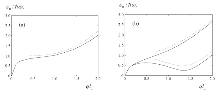
Being combined it with the fact that grows with for , the existence of this minimum results in a roton-maxon character of the spectrum as a whole [see Fig. 7(b)]. This type of the excitation spectrum in an infinite pancake trap can be understood as follows: For small in-plane momenta excitations have two-dimensional character and are phonons because dipoles being oriented perpendicular to the plane of the trap, repel each. On the other hand, excitations with large momenta have three-dimensional character and, hence, the repulsion between them is reduced. The excitation frequency therefore decreases with an increase of ,reaches a minimum, and starts to increase again as the excitations continuously enter the single-particle regime.
The roton minimum for close to found from Eq. (38) is located at , where , and is the harmonic oscillator length for the confined motion, and correspond to the excitation frequency
This minimum becomes deeper with increasing the density (chemical potential) or , and reaches zero at for . Excitations for larger values of have imaginary frequencies for , and, therefore, the condensate becomes unstable.
Eqs. (35) and (36) for various values of and were solved numerically in Ref. 82. The results for the excitation spectrum in the Thomas-Fermi regime are shown in Fig. 7, demonstrating a good agreement between numerical and analytical approaches.
For non-Thomas-Fermi condensates, the stability does not require as strong short-range repulsive interaction as in the Thomas-Fermi regime because of a large kinetic energy in the confined direction. The spectrum of excitations in this case also has a roton-maxon character, although the appearance of the roton minimum and the instability take place at smaller values of , see Ref. 82 for details.
Up to now, a roton-maxon dispersion was observed only in liquid He with strong interparticle interactions. Dipolar condensate provides the first example of a weakly interacting system with a roton-maxon excitation spectrum. This spectrum can be controlled and manipulated by changing the density, the strength of the confinement, and the short-range interaction, starting from the Bogoliubov-type spectrum, then creating the roton minimum, and finally reach the point of instability.
It is important to point out that the existence of the roton minimum with at a given for just below the point of instability is likely to indicate the existence of a new ground state presumably with a periodic density modulation. This is in contrast to the instability of condensates with attractive short-range interaction, which is driven by unstable long wavelength excitations resulting in local collapses. In this case the chemical potential is negative and not bounded from below such that no new ground state exists. In the Section 6 we will show that the excitation spectrum of a two-dimensional dipolar gas in the strongly interacting regime also has the roton minimum, and the system undergoes a liquid to solid quantum phase transition.
4 Weakly interacting dipolar Fermi gas
In this Section we discuss fermionic dipolar gases in the weakly interacting regime. Most of the discussion will be devoted to a single-component (polarized) dipolar gas with only brief mentioning some results available for two- and more component dipolar systems.
The crucial differences in the behavior of many-body fermionic systems as compared to bosonic ones are related to the Pauli principle: identical fermions are not allowed to be in the same quantum state. As a result, the many-body wave function of a single component Fermi gas should be antisymmetric with respect to permutations of the positions of any two particles. In the second quantization, this requires that the field operators and obey the canonical anticommutation relations
As a direct consequence, the wave function of a relative motion of two identical fermions is allowed to have components with only odd values, , of the angular momentum, and vanishes when the interparticle distance tends to zero. Therefore, the low-energy scattering of two identical fermions is insensitive to the short-range part of their interaction and is solely determined by the long-range dipole-dipole part . As a result, for a single-component polarized dipolar Fermi gas we can omit the contact term in Eq. (2), and the corresponding Hamiltonian then reads
| (39) | |||||
where is given by Eq. (1) and is the trapping potential (if present).
Another consequence of the Pauli principle is that the state of a many-body system of fermions at a low temperature is completely different from that for bosons. The average number of ideal fermions in a quantum state with the energy is given by the Fermi-Dirac distribution
where is the chemical potential, which depends on and, as usual, ensures the fixed total number of particles . The ground state () therefore corresponds to all quantum state with being completely completely occupied [], while the states with are are being empty []. The energy is called the Fermi energy and sets the typical energy scale a many-body system of fermions.
The ground state of an ideal homogeneous Fermi gas with corresponds to the so-called Fermi sphere: All quantum states with momenta below the Fermi momentum are occupied and the states with are empty. The states with momentum form a surface in the momentum space called the Fermi surface, which separates the filled and empty states. Semiclassical state counting provides the relation between the Fermi momentum and the density of a single-component homogeneous gas:
| (40) |
For a trapped Fermi gas we can establish the similar relation but between the local Fermi momentum and the local density of the gas ,
| (41) |
where
| (42) |
provided the chemical potential is much larger than the level spacing in the trapping potential . This condition corresponds to a large number of particle in the trap, most of them occupying high energy states of the trapping potential. The wave functions of these states are quasiclassical (see, for example, 89), and the calculation of the gas density results in Eq. 41, which is the essence of the local-density (Thomas-Fermi) approximation. This approximation is legitimate when the trapping potential changes slowly over the distances of the order of the average interparticle separation . For an ideal Fermi gas in a harmonic potential expression (42) gives
where is the Fermi momentum in the center of the trap and is the Thomas-Fermi size of the gas cloud in the -direction. The density of the gas in this approximation, according to Eq. (41), reads
| (43) |
where is the density in the trap center. The calculation of the total number of particle with the use of the above density distribution relates the chemical potential to the total number of particle and the parameters of the trap:
where .
For understanding the properties of the fermionic systems it is important to keep in mind that the ground state in the form of a filled Fermi sphere stores a large amount of kinetic energy. This guaranties applicability of the perturbation theory for dilute dipolar systems with . Another consequence is the improved stability of fermionic dipolar gases, as compared to the bosonic ones, against collapse due to the attractive part of the dipole-dipole interaction. This can be understood as follows: The energy per volume for a homogenous dipolar Fermi gas with density effectively attractive two-body interaction can be written as
where the first term is the kinetic energy of the filled Fermi sphere and the second term is the interaction energy with some numerical coefficient of the order unity. The first term scales as [see Eq. (40)] and provides an energy barrier between states with small and positive energy and collapsing states with and negative energy. Therefore, one expects the stability against collapse when the system is dilute: or, equivalently, , and instability in the dense system with when the interaction energy becomes comparable or larger that the kinetic energy. Applying this arguments to a trapped single-component dipolar Fermi gas, one expects to have a stable gas for or , where is the oscillator length and we use Eq. (43) to obtain . We provide more details on the issue of stability later.
4.1 Effects of dipole-dipole interactions.
When considering effects of interparticle interactions in Fermi systems, one has to keep in mind two possible scenarios depending on whether the properties of the system (the ground state and excitations) change continuously or abruptly when interactions are switched on. In the first case an interacting system is called normal Fermi liquid (in other words, belongs to Fermi liquid universality class) and has properties that are very much similar to those of an ideal Fermi gas. Of course, the interaction leads to appearance of new features (collective modes, for example), which are absent in a non-interacting gas, but for many applications the system can be considered as an ideal gas of fermionic non-interacting quasiparticles. For weak interparticle interactions, the properties of the interacting system can be obtained with the help of perturbation theory starting from the non-interacting Fermi gas. In the second scenario, the ground state and excitations of interacting system are qualitatively different from those of the non-interacting Fermi gas, and a system is in non-Fermi liquid universality class. This scenario is usually associated with breaking of some symmetries of an ideal gas: phase (or gauge) symmetry in a superfluid Fermi liquid or translational symmetry in a charge-density wave or crystal state. The new ground state cannot be continuously connected with the filled Fermi sphere (ground state of a non-interacting Fermi gas), and, therefore, one has to go beyond simple perturbative expansions to describe those states. It is important to mention that one does not necessarily need a strong interaction for the second scenario. For example, even an infinitesimally small attractive interaction results in a superfluid ground state. The smallness of the interaction in this case manifests itself in low (much smaller that ) critical temperature - the temperature above which the superfluid properties disappear and the system returns to normal Fermi liquid. In contrast, the charge-density wave state requires strong interaction, and this state disappears at temperature comparable or larger that when the gas is essentially classical.
As we will discuss below, depending on an experimental setup, both scenarios are possible in a polarized dipolar gas: A 3D polarized dipolar gas is in the superfluid state for low temperatures, , and in the normal state (Fermi-liquid) for . The state of a monolayer of polarized dipoles depends on temperature and relative angle between the dipole moments and the motion plane of molecules. For the perpendicular orientation of dipoles, the gas is in the normal state, but, starting from some critical tilting angle, becomes a superfluid at small enough temperatures . In both cases, the increase of the strength of the dipole-dipole interaction leads to the instability of the homogeneous state resulting to a collapse or formation of density-wave state with broken translational symmetry.
4.2 Normal (anisotropic) Fermi liquid state.
We begin with discussion of a normal Fermi liquid state of a dipolar fermi gas, which is a generic state for a fermionic dipolar gas at finite () temperatures, as well as for a purely repulsive (in a monolayer, for example) dipolar gas, in a weakly interacting regime . Following the original idea of Landau, an interacting normal Fermi system (Fermi liquid) can be described in terms of fermionic quasiparticles, which can be viewed as particles together with disturbances they produce in the system due to interactions with another particles (particles surrounded by particle-hole excitations) - dressed particles. In the ground state, the quasiparticles occupy all states with energies smaller or equal than the chemical potential forming a filled Fermi sphere (in a spatially uniform dipolar gas this corresponds to a deformed Fermi sphere in momentum space due to anisotropy of the dipole-dipole interaction, see below). Excited states are obtained by moving some quasiparticle from occupied states below to empty ones above - creation particle-hole excitations. The advantage of this description is that weakly excited states correspond to small number of particle-hole excitations near the Fermi surface and, hence, can be described using the dilute gas approximation. Note that, although we are talking about filled quasiparticle states inside the Fermi sphere, quasiparticles in the Fermi liquid are well-defined only in the vicinity of the Fermi surface where their energies are much larger than the inverse of their life-times due to decay via creation of particle-hole pairs. (In a weakly interacting gas the quasiparticles are well-defined for all momenta.) This is because the presence of occupied states below the Fermi energy strongly reduces the phase space volume for such processes, and, as a result, the life-time of quasiparticle near the fermi surface in a Fermi liquid are much larger than the corresponding time in a classical gas with the same interparticle interactions and density, . But those are quasiparticles we actually need to describe low-energy excitations of the Fermi system and its behavior at low temperatures and under weak external perturbations.
The change of the quasiparticle distribution (we assume here a spatially homogeneous gas) results in the change of the energy of the system
| (44) |
where is the quasiparticles energy (counted from the chemical potential ) and the second term describes the interaction between quasiparticles with being the Landau -function, which plays a crucial role in the Fermi-liquid theory, and can be either calculated perturbatively (if the gas is weakly interacting) or measured experimentally. Note that the function describes the change of the quasiparticles energy under the change of quasiparticle distribution as a result of their interaction,
which gives rise to Fermi-liquid corrections and make possible collective motion of quasiparticles (collective modes) even when collisions between quasiparticles can be neglected.
For states close to the Fermi surface (the boundary between occupied and empty states), the quasiparticle energy has the form
where is the Fermi momentum specifying the Fermi surface in momentum space, and is the effective mass. The Fermi momentum is related to the density in the same way as in the ideal gas, Eq. (40), reflecting the fact that numbers of particles and quasiparticles are equal, while the effective mass can be expressed in terms of the -function (see, for example Ref. 90). The compressibility , where is the chemical potential, is another important quantity, which can also be expressed in terms of -function. For a stable system one must have . Therefore, the knowledge of the compressibility as a function of system parameters provides us with stability conditions of the system against collapse. The stability of the system against possible deformations of the Fermi surface around its equilibrium form (Pomeranchuk criterion 91, 90]) can be obtained from the requirement that the change of the energy caused by this deformation, Eq. (44), is positive. In this way one can detect instabilities different from collapse, related to the nonuniform change of the Fermi surface.
The -function determines also collective modes in the Fermi liquid (Landau zero sound), which correspond to a collisionless coherent dynamics of particle-hole excitations. The simplest way to describe zero sound is to use a semiclassical (or Wigner) quasiparticle distribution function , which is the Fourier transform of a single-particle density matrix with respect to the relative coordinate,
and describes the local momentum distribution of particles at position . In the ground state of a spatially homogeneous system, corresponds to a filled Fermi sphere. For a thermal equilibrium state, the step function has to be replaced with the Fermi-Dirac distribution, .Time evolution of non-equilibrium distributions are described by the quasiparticle kinetic equation
| (45) |
where and the collision integral, which normally appears on the right-hand side, is set to zero assuming low temperatures, as discussed above. The solutions of this equation of the form with and are called Landau zero sound and described coherent motion of particle-hole pairs - propagation of a deformation of the Fermi surface. Generically, the solutions of this kind exist when is positive (for more details and exact criterion see, for example, Refs. 90). Note that the condition separates the zero-sound from the continuum of particle-hole excitations and ensures its long life-time. In the opposite case the energy of zero-sound waves would be inside the continuum of particle-hole excitations and, hence, the waves would rapidly decay into incoherent particle-hole excitations (Landau damping).
4.2.1 Anisotropic Fermi surface and single-particle excitations
Due to anisotropy of the dipole-dipole interaction, the Fermi surface in a dipolar gas is not a sphere any more and the modulus of the Fermi momentum depends on the direction. The effective mass becomes a tensor that can be defined from the relation between the Fermi momentum and fermi velocity , . This can easily be seen by using the following variational ansatz 92, 93
| (46) |
and find the variational parameter by minimizing the total energy of the system with the interaction energy calculated in the Hartree-Foch approximation:
| (47) |
where is the volume of the system and only exchange (Fock) term contribute to the dipole-dipole interaction energy because the direct Hartree contribution
where is the gas density, vanishes in a homogeneous gas as a result of angular integrations. It was found that so that the Fermi surface is deformed into a spheroid stretched along the direction of dipoles (prolate spheroid). These findings were supported by microscopic calculations in the spirit of Landau liquid theory in Refs. 94 and 95. The quasiparticle energy calculated from Eq. (47) reads
which corresponds to the following Landau -function for a spatially homogeneous gas
| (48) |
with only exchange contribution. Note that the condition of spatial homogeneity of the gas is essential for validity of Eq. (48). This is because the Fourier component of the dipole-dipole interaction in non-analytic for (the limit depends on the direction approaches zero). As a result, the direct (Hartree) contribution vanishes only in the spatial homogeneity gas, in which one has averaged over the direction of , which is zero. In an inhomogeneous gas, this is not the case and one also has the contribution of the direct dipole-dipole interaction, see, for example, Eq. (52) describing spatially inhomogeneous variations of the quasiparticle distribution.
Setting to zero gives the position of the Fermi surface in momentum space , where is a (radial) unit vector (direction) in momentum space. The chemical potential then has to be defined selfconsistently from assuming a fixed gas density :
For weak interaction one finds 94
where is the angle between and the -axis. This gives . The energy and the chemical potential are
and
After expanding the quasiparticle energy in the vicinity of the Fermi surface, , one finds 95 that the tensor of the effective mass has only longitudinal and and transverse components:
where is the polar angle unit vector and
Calculations for moderate strengths of the dipole-dipole interactions and finite temperatures were performed in Refs. 92, 94, 96 including the trapped case (Ref. 92), as well as 2D (monolayer) and 1D (tube) gases, and two-component dipolar gas (Ref. 95). We mention here only some details for a monolayer and refer to these references for more details.
In a 2D dipolar gas (monolayer), when the chemical potential is much smaller than the frequency of the transverse confining potential in the -direction, , the transverse wave function of particles is limited to the ground state wave function of the harmonic oscillator, such that , where is the in-plane vector. The corresponding effective 2D dipole-dipole interaction for the in-plane motion
| (49) | |||||
where is the confluent hypergeometric function and is the angle between the direction of dipoles (in the -plane) and the motion -plane, has the following Fourier transform
| (50) |
where with being the error function and is the angle between and the -axis. For one has
| (51) |
which is linear in . (Strictly speaking, expression (51) contains also a constant which depends on the regularization of the Fourier integral at the origin. This constant corresponds to a short-range inerparticle interaction and, hence, has no physical effect in a single component Fermi gas because all its contributions should vanish upon proper antisymmetrization. We therefore set this constant to zero.) Within the Hartree-Fock approximation one then obtains (assuming )
for the position of the Fermi surface, where now is the unit vector of direction in the -plane, and
for the longitudinal (along ) and transverse (perpendicular to ) components of the effective mass, respectively 95. Note that for (dipoles are perpendicular to the plane and, therefore, the system has rotational symmetry around the -axis) the deformation of the Fermi surface disappears and with .
4.2.2 Collective modes (Landau zero sound)
Collective modes in a dipolar gas can be studied on the basis of the kinetic equation, Eq. (45). For small deviation of the quasiparticle distribution from equilibrium of the form
the kinetic equation reduces to the following equation on the unknown function
| (52) |
where and the wave vector is assumed to be much smaller than , . In the Hartree-Fock approximation, the -function is , see comments below Eq. (48) and Refs. 94, 95. Eq. (52) was analyzed numerically for a 3D gas in Refs. 94 and 95, and in 2D gas in Refs. 95, 97. (Note that in a 2D gas – monolayer – the first term in the -function can be omitted following the arguments from the end of the previous section.) The results for the sound velocity in a 3D gas together with the propagation limit due to particle-hole continuum are shown in Fig. 8 as a function of the propagation angle (the angle between and the -axis).

They show that the collective mode can propagate only in the certain cone of directions around the direction of dipoles polarization. This is counterintuitive to some extend because this is the direction in which two dipoles attract each other; on the other hand in the perpendicular direction, in which dipoles repel each other and, hence, one would expect the existence of the collective mode, no zero sound is possible. This can be understood by noting that the zero-sound propagation is dominated by the exchange contribution, not direct one, and, therefore, the intuition based on the direct interaction does not work, see Ref. 94 for more discussions of this issue. The sound velocity depends strongly on both the propagation direction and interactions strength : It increases monotonically with for and becomes a non-monotonic in for , see Fig. 8.
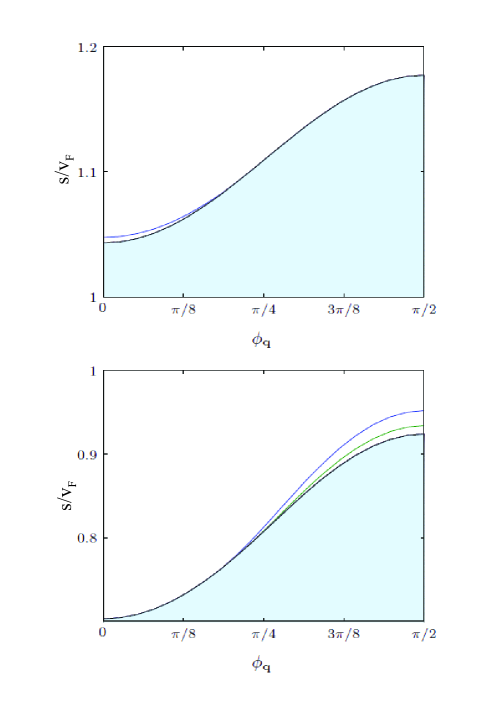
In a dipolar monolayer (quasi-2D gas), the situation is even more intriguing because the existence of zero-sound and the value of the sound velocity strongly depend on the propagation direction ( is the angle between and the -axis), on the tilting angle , and on the strength of the interaction. In this case, there is no collective modes if the tilting angle is smaller that some critical value that depends on the interaction strength, see Fig. 9.

This is again counterintuitive because the direct interaction for small tilting angles is purely repulsive (dipoles are almost perpendicular to the motion plane), and one would expect stable collective zero-sound modes. However, similar to the 3D case, the -function contains only exchange contribution, and this explains such peculiar behavior of collective modes. (The collective modes without exchange contribution were considered in Ref. 96.) Note also that with increasing the tilting angles from the critical one, the directions in plane, in which one has propagating zero-sound, changes from those around the projection of the dipole moment on the plane to those around the direction perpendicular to (when the polarization of dipoles approaches the plain), see Fig. 10.
Note, however, that the above results for collective modes were obtained with the -function in the lowest-order Hartree-Fock approximation, . Taking higher order terms into account can change the situation: As it was shown in Ref. 98 for the case of a 2D dipolar Fermi gas polarized perpendicular to the motion plane, , the inclusion of second order contributions to the -function results is the appearance of a stable zero-sound mode with the velocity .
4.3 BCS pairing in a homogeneous single-component dipolar Fermi gas.
The partial attractiveness of the dipole-dipole interaction opens the possibility for BCS pairing in a fermionic many-body dipolar system at sufficiently low temperatures. As we will see in this section, the pairing in dipolar systems has generically an unconventional character (different from a singlet isotropic -wave pairing as in a two-component fermionic system with an isotropic attractive interaction), and a superfluid state has many peculiar properties that are different from those of conventional superconductors. Indeed, the -wave (together with other even angular momentum) two-particle interaction channel is forbidden in a single-component Fermi gas by the Pauli principle. On the other hand, the angular part of the matrix element for the dipole-dipole interaction between the states with the angular momentum (-wave channel) and its projection on the -axis is negative (i.e. corresponding to an attractive interaction):
| (53) |
and, therefore, can lead to BCS pairing. (The matrix elements between the states with are positive.) It easy to see that this pairing should be anisotropic, reaching its maximum amplitude in the direction of dipolar polarization when two dipoles attract each other, and being zero in the perpendicular directions corresponding to repulsive dipole-dipole interaction. As we will see, the dominant contribution has -wave symmetry.
The Cooper pairing in a polarized single-component dipolar Fermi gas has been discussed in Refs. 99 and 100 within the BCS approach with the restriction to purely -wave pairing. An exact value of the critical temperature and the angular dependence of the order parameter for a dilute gas were found in Ref. 101.
After omitting the contribution of the short-range part of the interparticle interaction, as discussed above, the Hamiltonian of a homogeneous single-component polarized dipolar Fermi gas reads
| (54) | |||||
We considered the property of the system with this Hamiltonian in the dilute limit and at temperatures much smaller than the chemical potential (or the Fermi energy ), , relevant for Cooper pairing. In this case one can neglect the corrections to the chemical potential due to the dipole-dipole interaction because .
The BCS pairing corresponds to a nonzero value of the order parameter
which can be viewed as a wave function of Cooper pairs. because of anticommutativity of the fermionic field operators, changes sign under the exchange of particles forming a pair. As a consequence, the order parameter in momentum space
is also antisymmetric, . Because of the anisotropy of the dipole-dipole interaction, the angular momentum of the relative motion of two particles is not a conserved quantum number, but its projection on the -axis (in the considered geometry) does. We can therefore write in the form
| (55) |
where are the spherical harmonics and is the unit vector in the direction of the momentum . We keep in the sum only odd angular momentum following the discussion above and set in every term. This is because is a conserved and, following Eq. (53), only for one has an attractive interaction.
A nonzero order parameter and, therefore, the superfluid properties in the system appear for temperatures below some temperature which is the critical temperature of the superfluid transition. This critical temperature and the order parameter for temperatures below can be found from the gap equation 102,103 (we use the momentum representation and assume the order parameter to be real a real function of momentum )
| (56) |
where is the energy of single-particle excitations in the superfluid gas. The effective interparticle interaction is described by the function . Here is the Fourier transform of the bare dipole-dipole interaction potential :
| (57) |
with being the angle between the momentum and the -axis, and corresponds to corrections to the bare interparticle interaction resulted from many-body effects. The effective interaction describes all scattering processes in the system which transform a pair of particles with momenta and into a pair with momenta and . The leading process here is the direct scattering of the two particles on each other [the term ], while the many-body corrections describe processes of higher order in . The leading terms in are second order in (see Ref. 104) and correspond to scattering processes in which the two colliding particles interact with each other indirectly with an involvement of particle-hole excitations which they create in the system (see more details in Ref. 101). These processes are important even in the weakly interacting case (although they are of the second order in the small parameter) because they result in the pre-exponential factor in the expression for the critical temperature, see Eq. (59).
The gap equation (56) can be simplified for temperatures just below because for such temperatures the order parameter is small and, hence, the right-hand-sides of Eq.(56) can be expanded in powers of . The resulting equation
| (58) |
where and , is equivalent to the Ginzburg-Landau equation for a spatially homogeneous order parameter. .
Note that Eq. (58) always has the trivial solution which corresponds to a normal phase of the Fermi gas. The Cooper pairing is associated with a nontrivial solution of the gap equation (58) which exists for temperatures . To find the critical temperature , it is sufficient to keep only the linear term in the square brackets in the right-hand-side of Eq.(58) because for . The corresponding linearized gap equation allows also finding the momentum dependence of the order parameter. The absolute temperature dependent value of is determined by the nonlinear term in the right-hand-side of Eq.(58).
The result for the critical temperature reads (see Ref. 101 for details)
| (59) |
For temperatures close to , the anisotropic order parameter on the Fermi surface, , has the form
| (60) |
where
| (61) |
with being the angle between the vector and the -axis.
For momenta away from the Fermi surface the order parameter is
The dependence of the order parameter on the modulus of the momentum for several values of the angle is shown in Fig. 11.
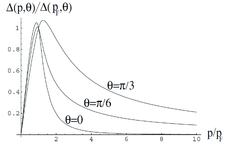
This momentum dependence of the order parameter in a dipolar Fermi gas is in contrast to that for pairing (both - and -wave) due to a short-range interparticle interaction, in which case the order parameter is a constant for momenta , where is the range of the interparticle interaction, and rapidly decays .
The anisotropy of the order parameter in the momentum space described by the function , see Eq. (60), provides another difference from the conventional -wave pairing, say in a two-component Fermi gas with a short-range intercomponent attractive interaction. As a result of this anisotropy, the gap in the spectrum of single-particle excitations in a dipolar superfluid gas depends on the direction of momentum : The gap reaches its maximum in the directions parallel to the direction of the dipoles (, ), while it vanishes in the direction perpendicular to the dipoles (). Similar anisotropic is expected in the properties of collective excitations, and, as a result, in the response of the dipolar superfluid dipolar Fermi gas.
The vanishing of the single-particle gap at (and arbitrary azimuthal angle , i.e. on the line on the Fermi surface ) results in the dependence of the specific heat of the gas at low temperatures (the contribution of collective excitations is proportional to ). Note that for the conventional -wave pairing, the low-temperature specific heat is determined by the contribution of collective modes (), while the contribution of single-particle excitations is exponentially suppressed.
The above mentioned properties of a superfluid dipolar Fermi gas is similar to those of the polar phase of superfluid liquid 3He. This phase, however, cannot be realized in experiments because it has higher energy than experimentally observed and phases (see, e.g. Ref. 105). Note that several heavy-fermion compounds in a superconducting state (for a review of superconducting phases of heavy-fermion compounds see, e.g. Refs. 106,107, and 108) also have lines of zeros of the order parameter on the Fermi surface and, as a consequence, the -dependence of the low-temperature specific heat (see, e.g. Ref. 109).
4.4 BCS pairing in a trapped single-component dipolar Fermi gas.
Similar to the bosonic case, the trap geometry strongly influences the BCS pairing in a polarized dipolar Fermi gas as a result of the dipole-dipole interaction. It is natural to expect that cigar-shaped traps are more favorable for pairing then pancake-shaped ones because the dipole-dipole interaction is on average attractive in the former case and repulsive in the latter one. As a result, the critical temperatures in cigar-shaped traps should be higher. This question was addressed in Refs. 110 and 86.
In a trapped gas, the BCS order parameter
| (62) |
depends on both coordinates and and not only on their difference as in the spatially homogeneous case, because the translational symmetry is broken by the trapping potential. To find the critical temperature in the trap, it is sufficient to consider the linearized gap equation:
| (63) |
with the kernel
where and are the eigenenergies (shifted by the chemical potential ) and the eigenfunctions of the single-particle Schrödinger equation in the trap
where is given by Eq. (13). Note that the gap equation (63) does not contain the mean-field Hartree-Fock corrections. They lead to unimportant change of parameters of the Hamiltonian (54) and, therefore are not relevant for pairing. The many-body contributions to the effective interparticle interaction which are also absent in Eq. (63) [compare with Eq. (56)], will be taken into account later.
The results of the analysis of Eq. (63) in Ref. 110 are the following. When (shallow nearly spherical trap), where is the critical temperature of the BCS transition in a spatially homogeneous gas with the density equals to the central density in the trap, it is convenient to perform the Fourier transformation with respect to the relative coordinate ,
where is the coordinate of the center of mass. The characteristic scale of the -dependence of is of the order of the Fermi momentum , while for the -dependence it is of the order of the size of the cloud , which is much larger than the typical size of pairing correlations (coherence length), . We therefor can write the order parameter on the local Fermi surface as , where the function obeys the equation (see Ref. 110 for details)
| (64) |
with , . The solution of this equation which is formally equivalent to the Schrödinger equation for a three-dimensional anisotropic harmonic oscillator, for the lowest eigenvalue gives the following expression
| (65) |
for the change of the critical temperature due to the presence of the trapping potential. According to this expression, the critical temperature in the trap is always smaller than that in the homogeneous gas. In the considered case we have but (weakly interacting gas). Taking into account that we see that the difference between and is small if is not very large.
The order parameter just below is given by the corresponding eigenfunction and has the Gaussian form
where
is the characteristic size in the -th direction. If again the quantity is not very large, we have , where is the Thomas-Fermi radius of the trapped gas cloud in the -th direction. This means that the pairing takes place only in the central part of the gas.
For a large number of particles the gas is in the Thomas-Fermi regime [Eq. (43)], and we have the following relation
between the total number of particle in the gas and the density in the center, where is the chemical potential. For a fixed and , this gives
| (66) |
where and is the trap aspect ratio. The function
is shown in Fig. 12.

The minimum of provides the optimal trap aspect ration (cigar shaped trap, as expected) for the highest critical temperature in the trapped gas with the fixed total number of particles and the density in the center [the critical temperature of the homogeneous gas as a function of is given by Eq. (59)]. The optimal value is a result of the competition between the anisotropic dipole-dipole interparticle interaction and the finite-size effects: The former favours larger (cigar shaped traps) while the latter, due to the zero boundary condition on the order parameter, acts on pairing destructively imposing an upper limit on .
Numerical solution of the linearized gap equation (63) for the case shows the existence of a critical trap aspect ratio for a given interaction strength and a number of particles . This critical aspect ratio corresponds to zero critical temperature, , such that no pairing is possible in traps with . Alternatively, for fixed values of the trap aspect ratio and the number of particles , BCS pairing takes place if the interaction parameter is large enough, . The existence of the critical values and can be understood as follows: Due to the fact that the order parameter changes sign when the direction of the -axis is reversed, single-particle states involved in forming the order parameter should have different (by an odd integer) quantum numbers . As a result, these states have different energies (the minimum difference is ) and can be paired only if the energy gain due to pairing (which is of the order of the critical temperature ) exceeds this difference. In the limiting case of an infinite pancake trap with the confinement only in the -direction, this results in the appearance of a critical trap frequency 86 with no pairing possible in traps with .
The dependence of the critical interaction strength on the trap aspect ratio for different is shown in Fig. 13.
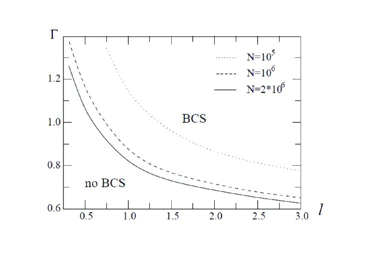
As expected, the critical interaction strength decreases with increasing . On the other hand, with increasing the number of particles , the interaction parameter becomes larger, , and the critical aspect ratio decreases.
The order parameter for a cigar shaped trap with (see Fig. 14) exhibits a non-monotonic behavior with the distance from the trap center. This is to be compared with a monotonic behavior of the BCS order parameter in a two component Fermi gas with a short-range attractive interaction 111-112 under similar conditions. (It should be noted, however, that an oscillating and highly non-monotonic behaviors of the order parameter in a two component Fermi gas was obtained in Ref. 113 in the regime of an intershell pairing .)
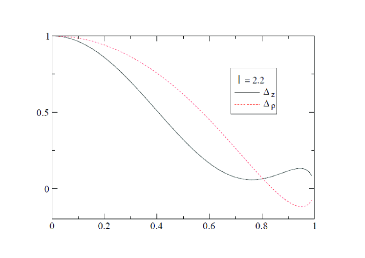
4.5 BCS pairing in a two component dipolar Fermi gas
Adding the second component in a dipolar Fermi gas opens the possibility for a singlet interspecies pairing (equivalent to the -wave pairing in a two component atomic Fermi gas) in addition to the triplet intraspecies pairing considered in Sec. 4.3, and competition between them. Assuming chemical stability of a mixture of two species of polarized dipolar particles with equal masses, concentrations, and dipole moments (a mixture of fermionic polar molecules with two different hyperfine states, for example), this problem was considered in Ref. 114. The corresponding Hamiltonian reads
where denotes two different species, the intraspecies interaction is the dipole-dipole one, , while the interspecies interaction for contains a short-range part in addition to the dipole-dipole interaction, , parametrized by the -wave scattering amplitude .
The order parameter of singlet interspecies pairing
in momentum space is now a sum of all partial waves with even angular momentum and zero azimuthal quantum number ,
| (67) |
The corresponding gap equation is similar to Eq. (56) with .
In the BCS approach, when one neglects many-body contributions including the deformation of the Fermi-sphere in momentum space, the critical temperature of the singlet superfluid transition is (see Ref. 114)
| (68) |
and the corresponding order parameter parameter on the Fermi surface reads [compare with Eq. (61)]
| (69) |
where is the largest positive root of the equation
The order parameter (69) is now a symmetric function under as it should be for a singlet pairing.
With the deformation of the Fermi surface taken into account, the problem was solved numerically (see Ref. 114 for details). It turns out that without contact interaction () the critical temperature of the triplet intraspecies pairing is always higher and, therefore, the system undergoes the transition into the triplet intraspecies BCS state, see Sec. 4.3. The ground state in this case is a mixture of two intraspecies triplet superfluids. However, switching on an attractive contact interaction () one can increase the critical temperature of the singlet pairing and make it larger than for the triplet one such that the ground state corresponds to an interspecies singlet superfluid. The critical value of as a function of and the corresponding phase diagram are shown in Fig. 15.

4.6 BCS pairing in a dipolar monolayer
Let us now consider the possibility for superfluid pairing in a polarized dipolar monolayer – a polarized single-component dipolar gas confined to a (quasi)2D geometry by a harmonic trapping potential , assuming , where is the Fermi energy of a Fermi gas with the 2D density . An important parameter of the problem is the angle between the -axis (normal to the 2D motion plane) and the direction of the dipole polarization, see Fig. 16.
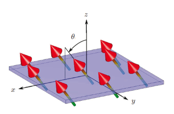
The effective 2D interaction between dipoles is given by Eqs. (49), (50), and (51). To see the possibility of BCS pairing, one has to look at the component in the -wave channel. Straightforward but lengthy calculations 115 show that it becomes negative when , and, therefore, the system becomes unstable against BCS pairing. Note that the critical value () is larger than the value () of the angle above which the dipole-dipole interaction has attractive directions in the -plane.
Due to the anisotropy of the effective interaction (for ), the azimuthal quantum number is no longer a conserving quantity and, therefore, the superfluid order parameter contains all odd harmonics in the azimuthal angle . In momentum space,
with the components coupled to each other through the gap equation. With only component taken into account, the problem was solved in Ref.115, in which is was also found that the Fermi surface deformation due to anisotropy of the effective interaction does not play any significant role in the pairing problem and only slightly decreases the critical angle when the strength of the interaction increases. This result was confirmed by the analysis of Ref. 97, in which all components of were taken into account. It appears that the critical angle remains practically the same, and higher components of with are visible only at angles very close to . For larger values of , one has such that the pairing has indeed the -wave character, .
The critical temperature for the BCS pairing reads 97
| (70) |
where
and
The two functions and in Eq. (70) describe deviations from the simplest BCS approach (with no account of the Fermi surface deformation): The exponent in Eq. (70) is simply the -wave component of the effective dipole-dipole interaction on the undeformed Fermi surface. These deviations result from many-body corrections to the interparticle interaction and Fermi-liquid effects, as well as from the second order contribution to the two-body quasi-2D scattering amplitude. The latter includes virtual transitions to intermediate states which are not necessarily limited to the ground state of the transverse confinement. The virtual transitions to excited states of the transverse confinement, together with many-body contributions (those include corrections to the interparticle interaction, Fermi surface deformation, and Fermi-liquid effects – effective mass), contribute to the function . The virtual transitions to the states with ground state motion in the transverse confining potential contribute to both functions and (see Ref. 97 for details). The latter transitions provide the second order Born term to purely 2D scattering amplitude on the effective potential (49), which has the so-called anomalous scattering contribution (see more discussions below) due to long-range power decay of the potential. This anomalous contribution gives rise to the function . Eq. (70) predicts a rapid growth of with increasing of the angle from the critical value , to the values of the order of tens of for realistic experimental parameters; see Fig. 17.
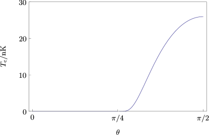
We obtain our results for the superfluid critical temperature using the mean-field approach. However, as it is well-known, this approach in two dimensions is only applicable at zero temperature, while at finite temperature the long-range order is destroyed by phase fluctuations and, therefore, the mean-field order parameter is zero. In this case, the transition into the superfluid phase follows the Berezinskii-Kosterlitz-Thouless (BKT) scenario 116, 117, and 118. In the weak coupling limit, however, as it was pointed out by Miyake 119, the difference between the critical temperature calculated within the mean-field approach and the critical temperature of the BKT transition can be estimated as and, therefore, small as compared to . As a result, our mean-field calculations provide a reliable answer for the critical temperature in the considered weak coupling regime .
Another interesting possibility to create a topologically nontrivial superfluid state in a monolayer was considered in Refs. 120 and 121, in which the authors consider a monolayer with fermionic dipoles oriented perpendicular to the plane () and use the RF-dressing technique discussed in Sec. 2.2.1 to create an effective (time-averaged) attractive potential . At short distances, the potential has a repulsive core that prevents low-energy particle from approaching each other and, therefore, suppresses inelastic collisions resulting in losses. The leading -wave 2D scattering amplitude for identical fermions was found 121 to be
| (71) |
where is the Bessel function, is the radial wave function of the -wave relative motion, the constant is determined by the behavior of the potential at short distances, and the length scale depends on the details of the RF-dressing (for BCS pairing has to be positive, for more details see in Ref. 121). The first term in Eq. (71) corresponds to the -wave Born amplitude for the potential while the second term contains both the anomalous scattering due to the dipole-dipole tail of the interparticle interaction and the short-range contribution.
For , the first term in Eq. (71) is negative and, therefore, leads to -wave superfluid transition. The most stable low-temperature -wave superfluid phase in 2D has symmetry, , because this is the only -wave superfluid phase with a non-zero energy gap on the entire Fermi sphere. The numerical solution of the gap equation 120, 121 shows that raises linearly for and approaches a constant for . The critical temperature reads
where
with the numerical coefficient determined by short-distance behavior of the interparticle interaction. Note that the value of the critical temperature is very sensitive to the short-range part of the effective potential and, by modifying it, can be varied within a few orders of magnitude. reaching the values of the order of tens of for realistic experimental parameters that correspond to the life-time of the system of the order of seconds; see Ref. 121 for details and discussions.
The resulting superfluid pairing spontaneously breaks time-reversal invariance (the degenerate time-reversal partner is the state). This phase belongs to the class of the so-called topological superconductors and can exist in one of two topologically distinct phases, depending on the sign of the chemical potential 122. The phase with is topologically trivial (may be continuously deformed to the vacuum state), while the phase with is topologically non-trivial ( cannot be continuously deformed to the vacuum) and has several very interesting properties. One of the most interesting of them is that the vortices in this superfluid carry localized zero-energy states, described by a Majorana fermion. These Majorana states obey non-Abelian exchange statistics 123, 124 and can possibly be used for topologically protected quantum information processing 125. In the considered case of superfluid state of dipoles in a monolayer, the chemical potential is positive, , and the resulting superfluid phase is topologically non-trivial.
4.7 BCS pairing in a bilayer dipolar system
The single-component fermionic bilayer dipolar system (see Fig. 18)
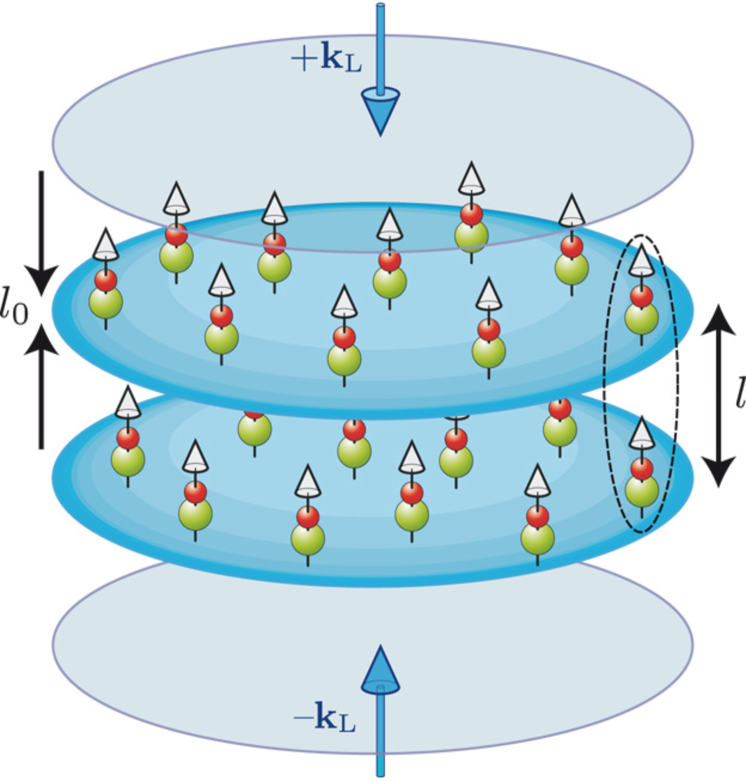
provides an example of a relatively simple many-body system in which an entire range of nontrivial many-body phenomena are solely tied to the dipole-dipole interparticle interaction with its unique properties: long-range and anisotropy. The long-range character provides an interparticle interaction in single-component Fermi gases inside each layer that otherwise would remain essentially noninteracting. For the considered setup, this intralayer interaction is always repulsive and gives rise to the crystalline phase for a large density of particles (see Sec. 2.2.3). More important, the long-range dipole-dipole interaction couples particles from different layers allowing them interact in the -wave channel that is dominant at low energies, allowing formation of bound states and BCS pairing 126, 127. The Hamiltonian of the system reads
| (72) |
where is the layer index, , with being the layer separation, with is the field operator for fermionic dipolar particles () on the corresponding layer , is the Laplace operator, is the confining frequency in each layer such that , and is the chemical potential. The last term describes the intra- () and interlayer () dipole-dipole interparticle interactions. Assuming a strong confinement, , where is the temperature, we can write and, therefore, reduce the Hamiltonian (72) to
| (73) | |||||
for a two-component fermionic field , , with shifted chemical potential . The intracomponent (intralayer) interaction coincides with in Eq. (49) for , and the intercomponent (interlayer) interaction is
| (74) |
The considered system is characterized by three characteristic lengths: the dipolar length , the interlayer separation , and the mean interparticle separation inside each layer with being the Fermi wave vector for a 2D single-component fermionic gas with the density . Therefore, the physics of the system is completely determined by two dimensionless parameters which are independent ratios of the above lengths. The first parameter (the ratio of the dipolar length and the interlayer separation) is a measure of the interlayer interaction strength relevant for pairing. In experiments with polar molecules, the values of the dipolar length is of the order of : for a with currently available one has (with for the maximum value ), and for with the tunable dipole moment from to in an external electric field the value of varies from to . For the interlayer separation these values of corresponds to . The second parameter measures the interlayer separation in units of the mean interparticle distance in each layer. This parameter can also be both smaller (dilute regime) and of the order or larger (dense regime) than unity for densities (for, example, for one has for ). The two parameters and determine the regime of interlayer scattering at typical energies of particles ( Fermi energy ), and their product, , as usual, controls the perturbative expansion in the system and, therefore, many-body effects.
The interlayer interaction has a very specific form resulting from the anisotropy of the interaction: Two particles from different layers attract each other at short and repel each other at large distances, respectively, as a result of different mutual orientations of their relative coordinate and of their dipole moments. A peculiar property of is
This means that its Fourier transform
| (75) |
vanishes for small ,
The potential well at short distances is strong enough to support at least one bound state for any strength of interlayer coupling. For a weak coupling between layers (), the bound state is extremely shallow and has an exponentially large size 127 (see also 128):
| (76) |
for the binding energy and
for the size, respectively. However, in the intermediate and strong coupling cases () the size of the deepest bound state becomes comparable with the interlayer separation:
and
respectively.
The specific properties of the interlayer potential (75): It decays exponentially for large momenta , while it is proportional to for , lead to different regimes of scattering and, therefore, of the BCS pairing, depending on the relation between and . This can be conveniently formulated in terms of the vertex function , where the arguments , ,and are independent of each other. This function satisfies the following integral equation 129
| (77) |
The 2D scattering amplitude , where is the angle between and , corresponds to with . The solution of this equation 127, 128 reads:
For , the leading contribution to scattering is given by the first Born term
| (78) |
For , the scattering is dominated by the second order Born contribution
| (79) |
which is momentum and energy independent and, hence, is equivalent to a pseudopotential ;
For , higher order contributions become important and one has to sum leading contributions from the entire Born series. The result of this summation is
| (80) |
where is the energy of the bound state from Eq. (76). This expression recovers the standard energy dependence of the 2D low-energy scattering and has a pole at , as it should be. The real part of the scattering amplitude, being zero at , changes from negative to positive values for and , respectively. Note that within the lowest order terms, a unique expression for the scattering amplitude can be written as
As one can see, the interlayer scattering amplitude is negative in the -wave channel [for the case this requires , which is realistic in the limit ]. This means that at sufficiently low temperatures, the bilayer fermionic dipolar system undergoes a BCS pairing transition into a superfluid state with interlayer -wave Cooper pairs, characterized by an order parameter with being the field operator in the momentum space, which is independent of the azimuthal angle , .
The analysis of the corresponding gap equation was performed in Refs. 126 and 127 (the latter includes many-body effects), and we present here only the results for the critical temperature in the experimentally most interesting case and such that (results for other cases scan be found in Ref. 127:
where
and being the modified Struve and Bessel functions, respectively,

The dependence of the function on for several values of is shown in Fig. 20.

We see that the critical temperature decreases very rapidly for due to the fast decay of the scattering amplitude. The optimal value of is around with the critical temperature reaching values of the order of for that corresponds to .
This BCS state with interlayer Cooper pairs occurs in the weak (interlayer) coupling regime when the size of the bound state is larger than the interparticle separation (in other words, the Fermi energy is larger than the binding energy). With increasing interlayer coupling, the BCS state smoothly transforms into a BEC state of tightly bound interlayer molecules when the interparticle separation is larger than the size of the bound state; see, for example, Refs. 126 and 130. Of course, the BEC regime and BEC-BCS crossover are possible only when the mean interparticle separation in each layer is larger than the distance between the layers.
Let us now discuss possible physical realizations of the interlayer pairing. In the experiments with polar molecules, the values of the dipolar length are of the order of : for a with currently available one has (with for the maximum value ), and for with a tunable dipole moment from to (in an external electric field ) the value of varies from to . For the interlayer separation of the order of few hundreds nanometers, the corresponding values of the parameter can be both smaller and larger than unity ().
The values of the parameter are also within this range for densities (for example, one has for and ). Note, however, that the optimal values of this parameter are around (see Fig. 20) and, hence, the optimum value of the interlayer separation is related to the density, which, in turn, should be large enough to provide a substantial value for the Fermi energy. For molecules at the density in each layer one has and . Therefore, the interlayer separation should be relatively small, , to meet the optimal conditions. For one then has (with current ), , and . Note that strictly speaking these values of parameters and do not correspond to the weak coupling regime considered in this paper, rather to the intermediate regime of the BCS-BEC crossover. However, based on the experience with the BEC-BCS crossover in two-component atomic fermionic mixtures, in which the critical temperature continues to grow when approaching the crossover region from the BCS side, we could expect that the above value of the critical temperature provides a good estimate for the onset of the superfluidity in the intermediate coupling regime.
4.8 Stability of fermionic dipolar systems
As we have already mentioned, a polarized homogeneous fermionic dipolar gas becomes unstable for strong dipole-dipole interaction (). Unfortunately, for this strongly interacting regime the usage of the Hartree-Fock approximation could not be rigorously justified. It is commonly accepted, however, that the Hartree-Fock method is able to provide a correct qualitative picture even in this regime, although its quantitative results should be taken with care.
The simplest way to get a quantitative insight into the instability region for a 3D dipolar gas is to use the variational ansatz (46) to calculate the compressibility. It turns out 93, 94 that the compressibility if a homogeneous gas becomes negative for signalling the instability of the gas leading to a collapse.
For a trapped gas with particles 92, the ansatz (46) for the momentum distribution has to be generalized to the ansatz for the Wigner distribution function
where is the position-dependent square of the Fermi momentum, and are variational parameters, , and with . Minimization of the energy with respect to the variational parameters , , and gives equilibrium density and local momentum distribution for a given value of the trap aspect ratio . The calculation of the compressibility shows that it becomes negative for any value of the trap aspect ratio provided the value of the parameter , which measures the strength of interparticle interaction, is sufficiently large. The dependence of the critical value of on the trap aspect ratio is shown in Fig. 21.
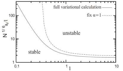
Note the found in Ref. 131 critical aspect ratio , below which the trapped gas is stable for any value of , is an artefact of the approximation used in this paper resulted from neglecting the deformation of local momentum distribution, see discussion in Ref. 92.
In a dipolar monolayer, the calculations of the compressibility in Ref. 115 shows that the collapse of the system takes place for for (dipoles are oriented parallel to the plane) but for rapidly increasing value of when the angle between the dipole polarization and the plane increases. More careful analysis of the both long wavelength (collapse) and finite wavelength (density wave) instabilities of a dipolar monolayer can be performed by looking at the stability of the collective modes: A collective mode becomes unstable when its frequency tends to zero. The corresponding equation valid for a general wave vector of the collective mode reads
| (81) |
where for our case. [Note that Eq. (52) follows from (81) after taking the limit and using the relation .] As a result, an instability occurs when the equation
| (82) |
has a non-trivial solution for some value of . Note that for (when only the direct interaction is taken into account and the exchange one is neglected), is -independent and Eq. (81) reduces to
| (83) |
where
is the 2D polarization operator. Eq. (83) is used to study long wavelength () plasmon oscillations in electrically charged systems (see, for example, 132). Although keeping only direct interaction in the long wave-length limit is legitimate for Coulomb systems (because of divergence of the Coulomb interaction, while the exchange one is finite due to non-zero momentum transfer, ), this approximation gives physically incorrect results in a Fermi system with a finite Fourier component of the interparticle interaction for small momentum transfer (like in the considered case of a dipolar monolayer). In this case, the direct and the exchange contributions are of the same order and keeping only the former results in unphysical results. Actually, for a short range interparticle interaction (with a momentum-independent Fourier component), the two contributions cancel each other, as it should be in a single-component Fermi gas. Similar considerations are also applied to the analysis of instabilities in a dipolar systems on the basis of Eq. (82): Keeping the exchange contribution in this equation is essential in order to obtain correct results consistent with fermionic statistics of particles.
For , Eq. (82) is equivalent to the Pomeranchuk criterion 91, 90] formulated in the framework of Landau Fermi-liquid. Numerical solution of this equation (for ) 97 shows that the instability of the system for corresponds to mostly isotropic with some addition of the quadrupole () deformation of the Fermi surface, i.e. to the collapse, that takes place for (see Fig. 22).

For , the leading instability corresponds to the -wave () deformation of the Fermi surface. However, this instability is unobservable because for these values of the tilting angle the system undergoes a density-wave instability at smaller values of 133, This instability corresponds to a non-trivial solution of Eq. (82) with finite and takes place for . For , the corresponding vector is along the -axis () and has the modulus that is twice larger than the Fermi wave-vector in the -direction, . For (isotropic case), the instability vector has no preferable directions and the system is believed to become unstable against formation of a crystalline state with the triangular lattice.
5 Dipolar multilayer systems
Let us now briefly discuss known results on dipolar multilayer systems. The stability against formation of inhomogeneous (density wave) phases in fermionic dipolar multilayer system was discussed in Ref. 134 for a particular choice of the tilting angle and in Ref. 135 for an arbitrary . The analysis of these papers show that inclusion of exchange interactions tends to stabilize the homogeneous state resulting in higher values of critical dipolar interaction strength as compared to the simple random-phase-approximation (RPA) approach. On the other hand, for multiple layers this critical dipolar interaction strength decreases with the number of layers.
Another interesting feature of multilayer systems of dipoles is the formation of many-body bound states in the form of a chain (or filament) made of one dipole in each layer 136, 137, 138, 139 (It was argued in Ref. 138 that bound states involving two molecules from the same layer do not exist.) The binding energy of such chains increases with the number of involved molecules (or layers). As a result, the ground state contains chains of maximum length, while at finite temperatures, the competition between entropy that favors shorter chains and energy preferring longer ones results in a non-monotonic dependence of the distribution on the length of the chains. For bosonic dipoles, quantum fluids of such self-assembled chains (dipolar chains fluid) and superfluidity of dipolar chains was considered in Ref. 136. For fermionic dipoles, the situation is even more interesting because chains with even number of dipoles are bosons, while with odd number of dipoles are fermions. In this case, even at zero temperature, there is an interplay between the Fermi statistics in the form of a Pauli principle giving rise to a finite kinetic energy of a filled Fermi sphere, and the binding energy, see Ref. 137, where a Bose-Fermi mixture of self-assembled noninteracting. chains was considered for the simple case of a three-layer system of fermionic polar molecules oriented perpendicular to the layers. For a more general case for both bosonic and fermionic dipoles, which also includes interactions between chains, see Ref. 139.
The superfluidity in fermionic dipolar multilayer systems was addressed in Ref. 140. The interlayer character of Cooper pairs in this case leads to the competition for pairing among adjacent layers resulting in a dimerized superfluid state as the ground state, in which the system can be viewed as a stack of bilayers with interlayer pairing correlations inside each bilayer and no such correlations between layers belonging to different bilayers. This state is characterized by a quasi-long-range superfluid order in every bilayer. At some finite critical temperature, this phase undergoes a phase transition into a dimerized ”pseudogap” phase with only short-range superfluid correlations. These correlations disappear above the second critical temperature, and the system is in the normal phase (see details and proposals for experimental detections of the phases and phase transitions in Ref. 140).
6 Strongly interacting dipolar gas
Strong correlations are at the core of a number of fundamental phenomena in
many-body physics, ranging from the formation of self-assembled ionic crystals
to exotic phases such as high-Tc superconductivity and spin liquids. The
regime of strong correlations between particles in a gas is generally obtained
when the strength of the inter-particle interactions becomes comparable to, or
larger than, the average kinetic energy. There are two main avenues to achieve
this regime of strong correlations: (i) the first is to decrease the kinetic
energy by placing particles on a lattice - which in the case of a dilute gas
has the effect of increasing the effective mass - and the second (ii) is to
increase the relative strength of interactions. In gases of dipolar particles
strong correlations can be achieved either way. In the following we first
discuss the phase diagram for dipoles confined to 2D with tunable interactions
(Sect. 6.1), and then we review several works on exotic
many-body phases for interacting dipoles trapped in optical lattice,
Sect. 6.2.
6.1 Two-dimensional dipoles: phase diagram.
The conceptually simplest example, although remarkably rich from a physics point of view, is a system of cold polar molecules in a DC electric field under strong transverse confinement. The setup is illustrated in Fig. 2(a). A weak DC field along the -direction induces a dipole moment in the ground state of each molecule. These molecules interact via the effective dipole-dipole interaction according to their induced dipoles, with . For molecules confined to the -plane perpendicular to the electric field this interaction is purely repulsive. For molecules displaced by the interaction becomes attractive, resulting in few-body and many-body instabilities. As discussed in Sect. 2.2, these instabilities can be suppressed by a sufficiently strong 2D confinement with the potential along , due to, for example, an optical force induced by an off-resonant light field 64.
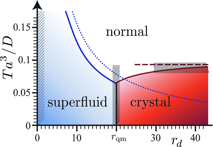
The 2D dynamics in this pancake configuration is described by the Hamiltonian
| (84) |
which is obtained by integrating out the fast -motion. Equation (84) is the sum of the 2D kinetic energy in the ,-plane and the repulsive 2D dipolar interaction
| (85) |
with a vector in the -plane [solid line in Fig. 3(a)]. The distinguishing feature of the system described by the Hamiltonian (84) is that tuning the induced dipole moment drives the system from a weakly interacting gas (a 2D superfluid in the case of bosons or a 2D Fermi liquid 142), to a crystalline phase in the limit of strong repulsive dipole-dipole interactions. This transition and the crystalline phase have no analog in the atomic bose gases with short range interactions modelled by a pseudopotential of a given scattering length.
A crystalline phase corresponds to the limit of strong repulsion where particles undergo small oscillations around their equilibrium positions, which is a result of the balance between the repulsive long-range dipole-dipole forces and an additional (weak) confining potential in the -plane. The relevant parameter is
| (86) |
which is the ratio of the interaction energy and the kinetic energy at the
mean interparticle distance . This parameter is tunable as a function of
from small to large. A crystal forms for , when
interactions dominate, which for a dipolar crystal is the limit of large
densities. This density dependence is different from that in Wigner crystals
with - Coulomb interactions, as realized e.g. with laser cooled trapped
ions 143. In the latter case
and the crystal forms at low densities. In addition, the charge is a fixed
quantitiy, while can be varied as a function of the DC field.
Figure 23 shows a schematic phase diagram for a dipolar gas of bosonic molecules in 2D as a function of and temperature . In the limit of weak interactions , the ground state is a superfluid (SF) with a finite (quasi-)condensate. The SF is characterized by a superfluid fraction , which depends on temperature , with . A Berezinskii–Kosterlitz–Thouless transition 116, 117 from the superfluid to a normal fluid occurs at a finite temperature , as expected in two dimensions. Recent numerical results in Ref. 144 obtained with an exact Path-Integral Monte-Carlo technique (PIMC) 145 have shown that the superfluid fraction , and thus , has a non-monotonic behavior as a function of the interaction strength , reaching a maximum of about at .
In the opposite limit of strong interactions the polar molecules
are in a crystalline phase for temperatures with , see Ref. 141. The configuration with minimal
energy is a triangular lattice with excitations given by acoustic phonons,
with characteristic Debye frequency . The intermediate strongly interacting regime
with has been investigated using several numerical, especially
quantum Monte-Carlo, techniques in
Refs. 64, 146, 147, 148, 149. Using
an exact PIMC technique, a quantum melting transition from the crystalline to
the superfluid phases has been determined to occur at a critical interaction
strength , 64.
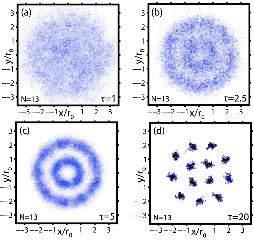
Confined geometries: The addition of an in-plane parabolic confinement of frequency as realized in experiments with magnetic or optical traps introduces a term in Eq. (84). The strength of interactions is now characterized by the dimensionless ratio , with the harmonic oscillator length. The physics of classical mesoscopic crystals with and dominant thermal fluctuations has been first discussed in the context of excitonic materials 151, 152, 153, 154. It was found that small dipolar clusters with particles confined to parabolic potentials may not crystallize in a triangular lattice, but rather arrange in shell-like structures. Finite- melting of these structures would usually proceed through two separate (non-sharp) transitions, corresponding to the loss of rotational and radial order.
Motivated by dipolar molecular and atomic gases, the focus has now shifted
towards the low-temperature regime of dominant quantum
fluctuations 152, 155, 156, 150, 157, 158, 159. For bosons, it was recently determined 156, 150 that
the quantum melting of mesoscopic crystals () into a superfluid
() is a sharp crossover involving two intermediate phases:
these are ring-crystals, with vanishing superfluid fraction, and mesoscopic
superfluids with a modulated (e.g., non-homogeneous) density. Snapshots of
quantum Monte-Carlo simulations for particles are shown in
Fig. 24 for all of these quantum phases.
Having determined the low-temperature phase-diagram both in the homogeneous
situation and in confined geometries, the remaining question is whether these
phases, and in particular the crystalline phase emerging at strong
dipole-dipole interactions, are in fact accessible with polar molecules. As
discussed in Sec. 2.2, stable 2D configurations for the molecules exist
in the parameter region where the combination of strong dipole-dipole
interactions and transverse (optical) trapping confines the particles’ motion
to the large distance region with , with the position of the saddle points in
Fig. 3(b) (white circles). For a given induced dipole the
ground-state of an ensemble of polar molecules is thus a crystal for mean
interparticle distances , where
corresponds to the
distance at which the crystal melts into a superfluid. For SrO (RbCs)
molecules with permanent dipole moment D (D), (nm), while can be several m. Since for
large enough interactions the melting temperature can be of
the order of several K, the self-assembled crystalline phase should be
accessible for reasonable experimental parameters using cold polar molecules.
Open questions: Remarkably, there are still important open questions
concerning the phase diagram of two-dimensional dipoles, and in particular the
order of the phase transitions between the solid and liquid phases at zero and
finite temperature. While as often happens 3 numerical results
are usually consistent with direct first order transitions, exotic
intermediate phases may occur in either case: (i) at finite an intermediate hexatic phase characterized by a short-range
positional and a quasi-long-range orientational (sixfold) order may exist
between the solid and the isotropic liquid phases. Evidence for this hexatic
phase, originally proposed by Kosterlitz, Thouless, Halperin, Nelson, and
Young 117, 160, 161, has been recently found
numerically in Ref. 162. (ii) At low-temperature theoretical
results suggest the presence of an intermediate microemulsion bubble
phase between the superfluid and the solid. First introduced in the context
of 2D electron gases in Si MOSFETs by Spivak and Kivelson 163,
and never observed so far (however, see below), a microemulsion should prevent
a first order transition in two dimensions. The observation of either phase
with cold dipolar gases would constitute a breakthrough for condensed matter theory.
Strong correlations can also occur in a weakly interacting dipolar gases
subject to rotation164, 165, 166, 167, 168, which,
as extensively reviewed in Ref. 32, represents
a key element to engineer effective magnetic
fields in ultracold atomic and molecular gases.
Strongly correlated phases similar to the Laughlin quantum Hall
states have been proposed in Ref. 165 for dipolar bosons and
for in Ref. 169 for dipolar fermions, while the transition from the Laughlin
liquid state to a dipolar crystal state was addressed in Ref. 170.
Recent work171 has now provided quantitative estimates for the realization
of Abelian and non-Abelian gauge fields with polar molecules.
6.2 Optical lattices
Hubbard Hamiltonians are model Hamiltonians describing the low-energy physics of interacting fermionic and bosonic particles in a lattice 172. They have the general tight-binding form
| (87) |
Here () are the destruction (creation)
operators for a particle at site in the internal state , describes coherent hopping of a particle from site to site
(typically the nearest neighbor), and
describes the onsite () or offsite () two-body interactions
between particles, with .
Hubbard models have a long history in condensed matter physics, where they
have been used as tight-binding approximations of strongly correlated systems.
For example, for a system of electrons in a crystal hopping from the orbital
of a given atom to that of its nearest neighbor, represents the
electron spin. A (fermionic) Hubbard model comprising electrons in a 2D
lattice with interspecies onsite interactions is thought to be responsible for
the high-temperature superconductivity observed in cuprates 173.
In recent years, Hubbard models have been shown to provide excellent microscopic descriptions of the low-energy physics of interacting bosonic and fermionic atoms trapped at the bottom of an optical lattice 174, 175. Since the interactions between cold atoms are short-ranged, in these systems Hubbard Hamiltonian typically have onsite interactions only [ in Eq. (87)]. This is readily shown for the simple case of single-species () bosonic atoms with contact interactions, such as 133Cs atoms prepared in their absolute internal (hyperfine, fine, …) ground-state, and trapped in the lowest band of an optical lattice. In the limit in which all energies involved in the system dynamics are small compared to excitation energies to the second band and neglecting the often-small overlap beyond nearest neighboring densities, the microscopic many-body Hamiltonian reduces to one of the form of Eq. (87) with nearest-neighbor hopping energy and on-site interactions 174 with
| (88) |
Here, is a complete set of single-particle basis functions, known as Wannier functions, which are linear combinations of exact solutions of the Schrödinger equation in the periodic optical potential (known as Bloch functions), and are localized at individual sites (here we focus on the lowest lattice band only). The optical lattice has a depth proportional to the intensity of the confining laser beams, with wavevector . In atomic systems, the Hamiltonian parameters in Eq. (6.2) can then be accurately controlled independently using external (optical, magnetic) fields: by increasing the intensity of the lattice laser light, decreases exponentially, while can be broadly tuned, e.g., by varying the scattering length using magnetic Feshbach resonances 3.
The resulting Bose-Hubbard Hamiltonian (BHH) has been extensively studied in condensed matter physics 176, 3. When the atom number is commensurate with the number of lattice sites, the BHH predicts a zero-temperature phase transition from a superfluid (SF) phase to a Mott insulator (MI) with an increasing ratio of the on site interaction (due to repulsion of atoms) to the tunneling matrix element . In the MI phase the density (occupation number per site) is pinned at an integer value = 1, 2, …, and the excitation spectrum shows a gap of the order of , corresponding to particle-hole excitations. When the density is not integer, the low-energy phase is superfluid for all strengths of the ratio . The associated phase diagram is sketched in Fig. 25 as a function of the chemical potential and the ratio , the lobes denoting MI regions of constant density.
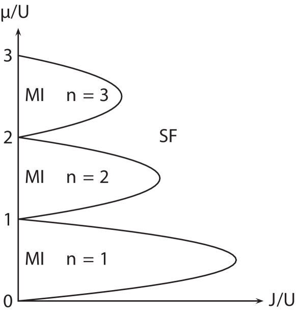
Spectacular experiments with ultracold atoms have lead to the first observation and characterization of this superfluid/Mott-insulator quantum phase transition for bosonic atoms 177, 178, 179, by looking at the interference of the expanded cloud, the measurement of the gapped excitations and the (lack of) conductivity in the Mott phase. Further experimental work with fermions may resolve the phase diagram of the fermionic Hubbard model in 2D by performing an analog quantum simulation of Eq. (87) with two-species cold fermions 180, 181, 182.
6.2.1 Dipoles on a 2D lattice monolayer
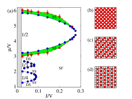
The long-range and anisotropic character of dipole-dipole interactions add to
the Bose-Hubbard model new possibilities to observe quantum phases of
fundamental interest. The simplest case is that of an ensemble of
single-species dipoles () which are all polarized
perpendicular to the lattice plane, resulting in isotropic in-plane
interactions. This adds to the BH Hamiltonian terms of the kind , with .
Extended Hubbard models have been extensively studied in literature. It has been predicted that in 2D lattices the presence of finite range interactions gives rise to novel quantum phases, like the charge-density wave (checkerboard), which is an insulating phase with modulated density, and the supersolid (SS) phase, with coexistence of superfluidity and of a periodic spatial modulation of the density, different from the one of the lattice 184. This latter phase has particularly interesting and storied history. First proposed in the context of the search for the groundstate of helium, it has been the subject of extended theoretical and experimental investigations for almost 40 years. While recent experiments may have spotted it in bulk solid helium, its very own existence in free-space, that is in the absence of an underlying periodic potential, is a matter of active research and debate. With few exact theoretical tools available in the strongly-interacting regime, quantum Monte-Carlo (QMC) methods have so far established SS behavior in free-space to be based on defects and disorder mechanisms, such as the presence of superfluid dislocations and grain boundaries 185. Crucially, any commensurate bulk solid (including 4He) should be insulating 186, notwithstanding recent theoretical proposals 187.
Several theoretical studies have demonstrated SS behavior in tight-binding
lattice
models 184, 188, 189, 190, 191, 183, 192, 193, 194, 195, 196, 197, 198. Model systems with nearest-neighbor (NN) or
next-neighrest-neighbor (NNN) interactions have been generally considered. The
variety of theoretical models and techniques which have been used has resulted
in a zoo of predictions. A general conclusion is that SS behavior seems to be
favored by finite-range interactions as well as finite on-site interactions,
. Quantum Monte-Carlo
methods have determined the SS to occur for the following models: i)
hard-core bosons (infinitely-large ) on a
triangular lattice with NN interactions only, for densities comprised between
; ii) hard-core bosons on a square lattice
with NN and NNN interactions for and between a
”star” and a ”stripe” solid at half filling; iii) soft-core
bosons (finite value of the ratio ) on a square lattice with NN and . Phase separation,
characterized by a negative compressibility, has been predicted to occur in
several models, for example in the latter case (iii) with NN interactions and
. However, its origin can be traced back to the finite-range
character of the interactions (NN) considered in that specific model, and thus
phase-separation may be expected to disappear in the case of the
infinite-range interactions considered below.
Dipolar atomic and molecular gases trapped in optical lattices can provide physical systems where the dynamics is microscopically described by extended-Hubbard Hamiltonians with long-range, anisotropic, interactions 199, with Hamiltonian parameters are tunable with external fields. In particular, polar molecules in optical lattices can provide for strong offsite dipolar interactions, of the order of hundreds of kHz, decaying with distance as . Due to these strong interactions, two molecules cannot hop onto the same site, and thus the particles may be treated as effectively ”hard-core” (soft-core particles may be realized with dipolar magnetic atoms). For a lattice of 2D polarized hard-core dipoles, the microscopic extended Bose-Hubbard Hamiltonian in the presence of long-range interactions is
| (89) |

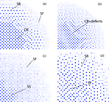
The phase diagram of Eq. (89) has been recently computed for 2D triangular 191 and square 183 lattices using exact QMC methods and no cutoff in the range of interactions. The zero-temperature phase diagram on a square lattice is shown in Fig. 26. For large enough , the low-energy phase is superfluid, for all . For finite , three main solid Mott lobes emerge with densities , 1/3, and 1/4. These are the checkerboard (CB), stripe, and star solids, respectively, the corresponding groundstate configurations being sketched in panels (b-d). Analogous to the standard Mott insulating phases of Fig. 25, these lattice solids at fractional filling factor exist in some low-tunneling region of the vs. phase diagram.
Interestingly, it was found that a supersolid phase can be stabilized in a broad range of parameters by doping the checkerboard and star Mott solids either with vacancies (removing particles) or interstitials (adding extra particles), in accordance with Andreev-Lifshitz’s scenario of defect-induced supersolidity 200. For example, a vacancy SS is present for densities , roughly independent of the interaction strength. In contrast to, e.g., case (iii) above, the long-range interactions prevent phase separation from occurring below filling in this microscopic model. This offers interesting prospects for the first observation of this exotic phase using polar molecules.
Both the solid/supersolid and supersolid/superfluid quantum phase transitions
are second-order. By increasing the SS melts into a featureless normal
fluid via a two-step transition, the intermediate phase being a normal fluid
with finite density modulations, similar to a liquid
crystal 183.
Devil’s staircase and metastable many-body states: The large Mott lobes
with , 1/3, and 1/4 are robust in the presence of a confining harmonic
potential and moderate finite , and thus are relevant to
experiments. Interestingly, for small-enough hopping the
low-energy phase is found to be incompressible ()
for most values of . This parameter region is labeled as DS in
Fig. 26 and it corresponds to a finite- version of the
classical Devil’s staircase. First discussed in the context of atomic
monolayers adsorbed on solids 201, the latter consists of a
succession of incompressible ground states, dense in the interval ,
with a spatial structure commensurate with the lattice for all rational
fillings 201, 202. This behavior, which has no
analogue for shorter range interactions, is shown in Fig. 27(a,b), where the particle density is plotted as a function of the chemical
potential . In the figure, a continuous increase of as a function of
signals a compressible phase, while a solid phase is characterized by a
constant . The main plateaux in panel (a) correspond to the Mott lobes of
Fig. 26, while the other steps are incompressible phases, with a
fixed, integer, number of particles, indicating the Devil’s-like
staircase. We will come back to this point in the discussion of
one-dimensional models.
Determining the exact groundstate geometry and periodicity of the solid for a
given set of Hamiltonian parameters in the DS region is however a
computationally daunting task, since i) for many rational fillings
[e.g. in Fig. 28(a)] it would require to consider system
sizes much larger than those accessible with reasonable numerical resources,
and ii) the long-range interactions determine the presence of
numerous low-energy metastable states 203, which for
finite can result in the presence of defects or in disordered structures.
The stability of low-energy metastable states has been thoroughly studied in
Refs. 203, 204, where it is found that especially in
larger lattices, two metastable configurations might differ by the occupation
of just a few lattice sites. Thus, because of the presence of these metastable
states, in an experiment it will be very difficult to reach the ground state
or a given metastable configuration. This is directly reflected in the
numerics: Figure 28 shows snapshots of the spatial density
distribution in the lattice in the presence of a realistic harmonic
confinement (shown is a single quadrant). Each circle corresponds to a
different site, and its radius is proportional to the local density. In panels
a) and b), is chosen such that particles at the trap center are in the
CB phase, with very small . The density profile shows a wedding-cake
structure, with concentric Mott-lobes with density and 1/4, analogous
to the shells with contact interactions 205, 206.
However, while the system parameters are the same in both figures, panel (a)
shows regular CB and star patterns, while in panel (b) extended defects are
present in the CB phase and the star is barely visible. This is due to the
different preparation of the states in panels (a) and (b). In fact, in panel
(a) temperature annealing of the system prior to taking the snapshot was
performed in order to eliminate defects, while this was not done in panel (b).
Defects in (b) reflect the existence of a large number of low-energy
metastable states, which are a direct consequence of the long-range nature of
the interactions.
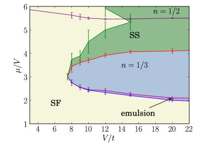
Additional exotic phases: Interestingly, the possibilities offered by
polarized dipoles in a 2D are not exhausted by the phases above. In
Ref. 191 first numerical evidence has been proposed for a
bosonic lattice version of the ”microemulsion”
phase 163 introduced in Sect.6.1 above,
for a system of polarized hard-core dipoles on a triangular lattice.
This is shown in Fig. 29, where an emulsion phase
is indicated as separating the Mott lobe at from a low-density
superfluid, suggesting a qualitative difference between the behavior of this
complex strongly-interacting system above and below the Mott lobe. In view of
future experiments with ultracold atomic gases with comparatively large
magnetic dipolar moments, such as Cr, Dy and Er atoms, it is an exciting
prospect to investigate how finite onsite interactions, which usually favor
supefluid and supersolid behavior, will modify this picture.
Fermi gases: A conclusive determination of the phase diagram of 2D fermionic dipoles has been so-far hampered by the lack of exact theoretical tools for the study of the strongly interacting regime. The experiments with dipolar gases have motivated several theoretical works, which use different approximate, often complementary, techniques. In analogy with Coulomb systems, for dipolar gases polarized perpendicular to the 2D plane (e.g., with isotropic in-plane interactions as discussed before) the existence of both crystal-like 207, 208, 209 and quantum liquid crystal phases 210, 211 (with interactions cut-off at NNN) has been recently discussed. In particular, using a mean-field-theory approach Ref. 207 has focused on determining the complex structure of phases and phase-transitions of charge-density waves with different lattice unit cells. References 212, 213 have discussed quantum liquid crystal phases, which may be obtained for anisotropic interactions. Analogous to the case of classical liquid crystals 214, these phases are classified as being nematic and smectic according to their symmetry breaking associated with the deformation of the Fermi surface as compared to the isotropic case. In the nematic phase, the rotational symmetry is broken so the typical Fermi surface has a cigar-like shape, i.e., it is stretched in one direction and shrunk in other directions. In the smectic phase the system is effectively in a reduced dimension, accordingly the Fermi surface is divided into disconnected pieces. Experiments with atomic and molecular dipoles will offer an enticing opportunity to test these predictions.
6.2.2 Polarized dipoles on a bilayer optical lattice
As discussed in Sect. 3 above, polarized dipoles trapped in a bilayer configuration can form a paired superfluid phase (PSF), which originates from the interlayer attraction due to dipole-dipole interactions, when tunneling between the two layers is suppressed. The addition of an in-plane optical lattice in the two layers makes this situation even more rich from a physical point of view: in Ref. 215 it was shown that the presence of strong enough intra-layer repulsion and inter-layer attraction for bosonic particles allows for the realization of a novel phase, named a pair-supersolid phase (PSS), which is defined as a supersolid phase of composite particles. Using a model Hamiltonian with finite on-site intra-layer interactions and NN intra-layer interactions and within a mean-field analysis, it was shown that the existence of the PSS phase relies on second order tunneling of (composite) dipoles in parameter regimes close to insulating Mott phases of (composite) dipoles, similar to the discussion of Sect. 6.2.1 above. One example is given in Fig. 30. The existence of this exotic phase had been previously discussed for anisotropic models 192, but no evidence was found. It remains an open question whether exact (e.g., QMC) calculations will confirm this prediction for realistic models with long-range interactions and, e.g., onsite hard-core constraint.
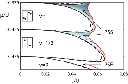
6.3 Advanced Hamiltonian design with polar molecules
The quantum phases of Sect. 6.2.1 are based on interactions of the dipole-dipole type, see Eq. (1), and are thus present for any dipolar gas. For polar molecules, the techniques described in Sect. 2.2 for modifying the shape of interaction potentials allow for an advanced engineering of microscopic Hamiltonians. This offers new opportunities to explore exotic many-body phases in these systems. In the following we review recent progress by discussing situations where pure three-body effective interactions can dominate the dynamics (Sect. 6.3.1), and the use of internal degrees of freedom for each molecule in addition to rotational ones can provide toolboxes for the simulation of condensed matter models of interest, including exotic lattice spin models (Sect. 6.3.2).
6.3.1 Three-body interactions
In Sect. 2.2 techniques were introduced for the modification of the shape of the effective interaction potentials using external DC electric and AC microwave fields coupling rotational excitations of the molecules. In particular, for a circularly polarized AC field the attractive time-averaged interaction due to the rotating dipole moments of the molecules has been shown to allow a strong reduction, and even a cancelation, of the total dipole-dipole interaction. In a dense ensemble of molecules this can lead to the realization of systems where the effective three-body interaction of Eq. (5) dominates over the two-body term and determines the properties of the system in the ground state. We note that, as always, direct particle-particle involve two particles only, while few-body interactions emerge as an effective low-energy interaction after the high-energy degrees of freedom are traced out.
Model Hamiltonians with strong three-body and many-body interactions are strong candidates for exhibiting exotic ground state properties. This is exemplified by the fractional quantum Hall states described by Pfaffian wave functions which appear as ground states of a Hamiltonian with three-body interactions 216, 217, 218. These topological phases support anyonic excitations with non-abelian braiding statistic. The possibility of realizing a Hamiltonian where the two-body interaction can be manipulated independently of the three-body term has been studied in Ref. 219. There, it is shown that a stable system of particles interacting via purely repulsive three-body potentials can be realized by combining the setup above with a tight optical confinement provided by an optical lattice. The latter ensures collisional stability of the setup and defines a characteristic length scale (the lattice spacing) where an exact cancelation of the two-body term can occur. The resulting extended Hubbard-like Hamiltonian has the form
| (90) |
where is an offsite three-body term. The latter is tunable independently of the two-body term , to the extent that it can be made to dominate the dynamics and determine the properties of the system in the ground state. This is in contrast to the common approach to derive effective many-body terms from Hubbard models involving two-body interactions, which are obtained in the perturbation limit, and are thus necessarily small 220.
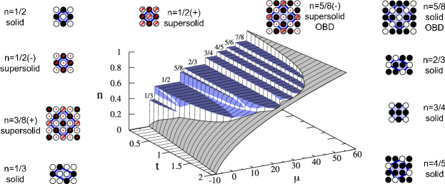
The phase diagram for bosonic particles on a 2D lattice with three-body interactions has been recently investigated in Ref. 221, where a rich variety of superfluid, solid, supersolid and phase separated phases have been found. In particular, several solid phases at fractional filling factor are found to evolve upon doping into supersolid phases with complex spatial structures. For example, the checkerboard supersolid at filling factor , which is unstable for hardcore bosons with nearest neighbor two-body interaction, is found to be again stable in a wide range of tunneling parameter, similar to the case of pure dipolar interactions discussed above.
6.3.2 Lattice Spin models and quantum magnetism
Lattice spin models are ubiquitous in condensed matter physics where they are used to describe the characteristic behavior of complicated interacting physical systems. Recent works have focused on realizing effective spin Hamiltonian for the simulation of lattice spin models of fundamental interest in condensed-matter, obtained by considering several internal states of each molecule.
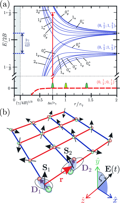
Reference 223 has shown that cold gases of polar molecules
can be used to construct in a natural way a complete toolbox for any
permutation symmetric two spin- (qubit) interaction, based on techniques
of interaction engineering which are extensions of those discussed in
Sect. 2.2. The main ingredient of this (and related) proposal is the
dipole-dipole interaction: it couples strongly the rotational motion of the
molecules, it can be designed by means of microwave fields, and it can be made
spin-dependent, exploiting the spin-rotation splitting of the molecular
rotational levels.
The basic building block in Ref. 223 is a system of two polar molecules strongly trapped at given sites of an optical lattice, where the spin- (or qubit) is represented by a single unpaired electron outside a closed shell of a heteronuclear molecule in its rotational ground state, as provided e.g. by alkaline-earth monohalogenides. Rotational excitations are described by the Hamiltonian
| (91) |
with the rotational angular momentum of the nuclei, and the dimensionless electronic spin (assumed to be in the following). Here denotes the rotational constant and is the spin-rotation coupling constant. The typical values of are a few tens of GHz, and is usually in the hundred MHz regime. The interaction describing the internal degrees of freedom is , where is the dipole-dipole interaction.
The molecules are assumed to be trapped in the optical lattice with a separation , where the dipole dipole interaction is . In this regime the rotation of the molecules is strongly coupled to the spin and the excited states are described by Hunds case (c) states in analogy to the dipole-dipole coupled excited electronic states of two atoms with fine-structure. Thus, while the two-particle ground states are essentially spin independent, effective spin-dependent interactions in the groundstates can be obtained by dynamically mixing dipole-dipole coupled excited states into the groundstates using a microwave field with properly-chosen polarization, frequency and Rabi-frequency , which is tuned near resonance with the transition.
The effective interactions in the lowest-energy states are obtained by diagonalizing the potential, as described in Sect. 2.2. In second order perturbation theory they read
| (92) |
where are ground states for two molecules with and are excited eigenstates of with and with excitation energies . The reduced interaction in the subspace of the spin degrees of freedom is then obtained by tracing over the motional degrees of freedom. For molecules trapped in the ground motional states of isotropic harmonic wells with rms width the wave function is separable in center of mass and relative coordinates, and the effective spin-spin Hamiltonian is .
The effective Hamiltonian Eq. (92) can in general be rewritten as 223
| (93) |
where and is a real symmetric tensor. Equation (93) describes a generic permutation symmetric two qubit Hamiltonian. The components describe a pseudo magnetic field which acts locally on each spin and the components describe two qubit coupling.
For a given field polarization, tuning the frequency near an excited state induces a particular spin pattern on the ground states. These patterns change as the frequency is tuned though multiple resonances at a fixed intermolecular separation. For example, the anisotropic spin model can be simulated using three fields: one polarized along tuned to , one polarized along tuned to and one polarized along tuned to . The strengths can be tuned by adjusting the Rabi frequencies and detunings of the three fields.
Of particular interest is the possibility of realizing highly anisotropic spin models such as the following one
| (94) |
which was first introduced by Douçot et al. 224 in
the context of Josephson junction arrays. This model (for )
admits a 2- fold degenerate ground subspace that is immune to local noise up
to -th order and hence is a good candidate for storing a topologically
protected qubit for applications in quantum computing. Other Hamiltonians that
can be realized include the famous Kitaev model.
References 225, 226, 227 have recently focused on the realization of tunable Heisenberg-type models for unit filling of the optical lattice. Effective spin degrees of freedom are encoded in internal, e.g. rotational, states of the molecules, and molecular interactions are tuned by a combination of DC and AC fields, using techniques similar to those of Sect. 2.2. In Refs. 226, 227 it is found that doping the lattice with vacancies (that is, removing particles from a few sites) leads to a tunable generalization of the so-called model, which is relevant in the context of high-temperature superconductivity 228. Typical Hamiltonian terms which are found in addition to Eq. (87) are of the form
| (95) | |||||
| (96) |
where the operators , , and are spin-1/2 angular momentum operators on site describing a two-level dressed rotor degree of freedom (e.g., the lowest two states of the molecule in the presence of a DC electric field along ), and satisfying . By intuitively thinking of the ground state as a (classical) dipole oriented along the DC field (i.e. ) and of the excited state as a dipole oriented against the DC electric field (i.e. ), the terms , , and derive from re-writing the direct dipole-dipole interaction, while the term comes from the transition dipole moment , describing the exchange of a microwave excitation between the molecules. One difference with the derivation of the effective spin models of Ref. 223 described above is that dipole-dipole interactions in Eq. (96) are used in first order, rather than second order, which can allow for stronger interactions.
We note that the design of extended Hamiltonians with terms as in Eq. (96) is in fact a hot topic of research in atomic and molecular systems: for example, Refs. 229, 230 have discussed the derivation of similar terms for trapped neutral atoms and molecules at unit filling, while Refs. 231, 232 have focused on ionic particles. The case is also studied in the context of molecules in Ref. 233. In Ref. 234, a similar Hamiltonian describes the dynamics of exciton-like interactions with impurities in gases of polar molecules. There, the authors considered first a clean system with one particle per site, subject to a very deep optical lattice potential in order to prevent particle tunneling: in this regime, dipole-dipole interactions induce collective excitonic modes, in sharp contrast with individual rotational excitations of short-range interacting atoms. After substituting a small number of initial components with a different kind of molecule still strongly confined by the optical potential, the system displays an exciton-impurity interactions between the original excitonic modes and the new particles, which may be treated as effective impurities, leading to a disordered background potential with both diagonal and off-diagonal contributions. Such a setup represents an ideal platform to investigate the effect of disorder and interaction induced localization in excitonic gases in both 1, 2 and 3D.
Reference 235 has considered an ensemble of
molecules in the rotationally ground state trapped on an optical lattice and
have shown that collective spin excitations can be controlled using external
electric and magnetic fields, in the context of the formation of Frenkel
excitons 236, 237. This system may be used for the quantum
simulation of spin excitation transfer in many-body crystals without phonons.
In Ref. 238 a similar Hamiltonian has been studied in the context
of molecular self-assembled crystals for quantum memory applications.
The inclusion of more internal states for the particles, such as hyperfine levels, offers extensions to spin systems with larger spin 239, 225, 226, 227. For example, the design of a large class of spin-1 interactions for polar molecules has been shown in Ref. 239, which allows e.g. for the realization of a generalized Haldane model in 1D, using a strategy of interaction-engineering similar to those described above. Recent work in Ref. 225 has started exploring the non-equilibrium dynamics of molecules trapped in optical lattices in the presence of several internal states, including, e.g., the rich hyperfine structure often present in the ground state rotational manifolds. In particular, it was shown that the number of effective degrees of freedom participating to the dynamics may be indeed dynamically changed for each molecule using external electric and magnetic fields, similar to the discussion above. This raises interesting prospects for the study of non-equilibrium dynamics in these complex systems. In section Sec. 7. below, we discuss some of the intriguing scenarios opened up in the many-body context by the accurate fine-tuning of interactions presented here, for the particular case of polar molecules trapped in 1D.
6.3.3 Hubbard models in self-assembled dipolar lattices

In Hubbard models with cold atoms or molecules in optical lattices there are no phonon degrees of freedom corresponding to an intrinsic dynamics of the lattice, since the back action on the optical potentials is typically negligible. Thus, the simulation of polaronic materials 240 where the presence of crystal phonons affects strongly the Hubbard-like dynamics of particles remains largely a challenge. References 241, 242 have shown that a self-assembled floating lattice of molecules as discussed in Sect. 6.1 can provide a periodic trapping potential for extra atoms or molecules, whose dynamics can be described in terms of a Hubbard model with phonons, the latter corresponding to vibrations of the dipolar lattice.
The Hamiltonian for extra atoms or molecules in a self-assembled dipolar lattice is
| (97) |
Here, the first and second terms define a Hubbard-like Hamiltonian for the extra-particles of the form of Eq. (87), where the operators () are destruction (creation) operators of the extra-particles. However, the third and fourth terms describe the acoustic phonons of the crystal [ destroys a phonon of quansimomentum in the mode ] and the coupling of the extra-particles to the crystal phonons, respectively. Tracing over these phonon degrees of freedom in a strong coupling limit provides effective Hubbard models for the extra-particles dressed by the crystal phonons
| (98) |
The hopping of a dressed extra-particle between the minima of the periodic
potential occurs at a rate , which is exponentially suppressed due
to the co-propagation of the lattice distortion, while offsite
particle-particle interactions are now a combination of
direct particle-particle interactions and interactions mediated by the
coupling to phonons, as given by polaronic dynamics 243.
Figure 33 shows two implementations of this idea in two- and
quasi-one-dimensional configurations, [panels (a) and (b-c), respectively].
The distinguishing features of this realization of lattice models are the
tunability of interactions among crystal dipoles, and of the particle-phonon
couplings. In addition, the lattice spacings are tunable with external control
fields, ranging from a m down to the hundred nm regime, i.e. potentially
smaller than for optical lattices. Compared with optical lattices, for
example, a small scale lattice yields significantly enhanced hopping
amplitudes, which set the relevant energy scale for the Hubbard model, and
thus also the temperature requirements for realizing strongly correlated
quantum phases. Phonon-mediated interactions can be quite long-ranged,
decaying with distance as in 1D.
7 Dipolar gases in one- and quasi-one dimensional geometries
In reduced dimensionality, the effects of quantum fluctuations are so relevant that the standard Fermi-liquid picture breaks down due to the emergence of several strongly correlated states of matter. The addition of interaction with long-range, anisotropic tail such as the dipolar one leads to the stabilization of very rich phase diagram in both purely 1D systems and coupled ones such as ladders and planar arrays. In the following, we will first review the basic physics of the single tube configuration and then illustrate recent results on two-leg and multi-leg ladders.
7.1 Dipolar gases in a single tube
We now consider a system of dipolar particles confined in a one dimensional (1D) geometry by a sufficiently deep optical lattice with frequency , so that their dynamics is purely 1D. In order to ensure collisional stability, we will consider all dipole moments aligned perpendicularly to the wire direction by an external field in such a way that the inter-particle interaction is always repulsive. Defining the mass of the particles and the strength of the dipolar interaction, a proper description for, e.g., a gas of polar molecules in the long-distance regime (see Sec. 2) is encoded in the following model Hamiltonian:
| (99) |
where are annihilation/creation operators with bosonic or fermionic statistics. For a polar molecule gas, , where is the vacuum permeability and the dipole moment induced by a DC electric field. After a proper rescaling of all quantities, one can see that the only relevant parameter is the ration between the dipolar length and the linear density and, as such, we expect all thermodynamic properties to depend only on . While statistical properties are expected not to play a major role in this setup since bosons are subject to an effective hard-core condition due to the infinite short-distance repulsion, some properties of the system are still affected by statistics; thus, we will at first consider a bosonic gas, and then comment on the fermionic case at the end of the section. Qualitative features of Eq. (99) are obtained using the bosonization technique, which allows to map the original interacting problem into a free one via the identities 244, 245, 246, 247:
| (100) |
| (101) |
Here, the field and represent density and phase fluctuations of the original field, and satisfy bosonic commutation relations . As long as the long-range tail of the interaction potential decays faster than Coulomb-like interactions248, 249, , as in the dipolar case, the Hamiltonian in Eq. (99) is mapped into the so-called Tomonaga-Luttinger liquid (TLL)244:
| (102) |
which is a purely quadratic Hamiltonian with a linear dispersion relation at small momenta, ; the excitations in the system are sound waves of the density with correspondent sound velocity , whereas the factor , known as Tomonaga-Luttinger liquid parameter, is related to the compressibility of the system via , and in Galilean invariant systems satisfies . The TLL picture captures the entire low-energy physics of the original model, and represents the substitute of the Landau-Fermi liquid scenario in 1D; analogously, the parameters play a similar role to the Landau parameters in higher dimensions. In addition, the long-distance decay of correlations functions is completely captured by , so that after the bosonization mapping one gets:
| (103) |
for the one-body density matrix, also known as superfluid (SF) correlation, and
| (104) |
for the correlated part of density-density, or charge-density-wave (CDW), correlation function. The possibility of qualitatively describing the asymptotic decay of correlations is remarkable. Since spontaneous symmetry breaking is not allowed in many 1D models because of the Mermin-Wagner-Hohenberg theorem 250, 251, correlation functions encode the necessary information to distinguish between different phases in low dimensional geometries; the slowest decaying correlation is usually referred to as dominant order, corresponding to the more diverging susceptibility in the system 246, 245. From Eq. (103) and (104), we thus expect a transition from dominant SF correlations to CDW ones at a precise value of the TLL parameter, , where the two decay exponents coincide.
While in principle all information regarding the quantum phases in 1D is encoded in the LL parameters, the bosonization techniques sketched above do not in allow in general to establish a relation between the microscopic quantities in Eq. (99) and , as the latter has to be regarded as a phenomenological parameter to be determined by comparisons with experiments or numerical results. Before discussing the general case, let us comment on some relevant situations. In the weakly interacting limit, , the dipolar interaction is relevant only at very short distances, and thus the system behaves very similarly to a Tonks-Girardeau gas 252, 253, for which ; as such, we expect in the weakly interacting regime. In the strongly interacting case, , it has been noticed in Ref. 254, 255 that, approximating the system as a classical crystal where particles are quasi-localized at equally spaced distances, one has an energy per particle (where is the Riemann zeta function), and deriving from it the compressibility , the resulting TLL parameter in the strong coupling regime reads:
| (105) |
Away from these two limits, the mapping of K into the microscopic parameters of Eq. (99) has to be performed using non-perturbative techniques. Numerical QMC simulations based on both reptation, diffusion and Worm algorithm have been performed 254, 256, 257, allowing to estimate the TLL parameter from the so called static structure factor
| (106) |
and from the long-distance decay of (see Fig. 36). Moreover, QMC also allows to quantitatively estimate the momentum distribution
| (107) |
which is directly measurable in experiments, and, according to TLL theory, displays a clear signature of the SF/CDW transition as the typical peak of quasi-condensation at disappears just across the phase boundary between the SF and CDW phases. Typical QMC results for are shown in Fig. 36 just across the phase boundary, as can be argued from the sharp decrease of when the interaction is increased. Moreover, analytical results obtained through approximate methods lead to the following expression 258:
| (108) |
which compares favorably with numerical simulations, as can be seen in Fig. 36, and recovers the limit in Eq. (105) at strong coupling.
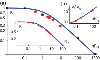

Let us briefly discuss the relationship between a dipolar interacting gas and a bosonic one with a contact repulsive interaction, the Lieb-Liniger model 259. Besides sharing the same low-energy universality class (TLL) which allows to describe thermodynamical properties of both systems on the same footing, there are quantitative and qualitative differences between the two cases. The former is related to the very different domain spanned by the TLL parameter, that is, for dipoles, whereas for contact interactions. In addition to the momentum distribution, such a feature can in principle be detected by investigating the so called breathing mode, which, as shown in Ref. 260, displays a remarkably different behavior. Qualitative differences are not only captured by to the fact that non-local interactions allow to cross the SF-CDW transition; another very important feature is the response to a periodic potential, which changes qualitatively when considering non-local repulsion, as we will see in the next section. As a final remark, we resume the main differences between bosonic and fermionic dipolar wires: while the TLL picture remains quantitatively the same between the two, single particle correlation functions are slightly different from Eq. (103), and, since no superfluid instability may occur, the dominant correlation in the fermionic case is always a CDW.
7.1.1 Bosonic and fermionic gases in an shallow optical lattice
The effects of dipolar interactions become even more relevant in the presence of external perturbations such as an underlying periodic potential, as realized, e.g., by an optical lattice along the direction of the tube 3. In this configuration, long-range interactions compete with both kinetic energy and the periodic lattice potential, which in 1D has the form 261:
| (109) |
where is the laser wavelength, the dimensionless depth of the lattice potential, and the recoil energy. In the limit of a very shallow lattice, , the periodic potential may be considered as a perturbation on the TLL Hamiltonian, Eq. (102), and its effects may be investigated using a sine-Gordon description 258, 261, 246. The phase diagram, and thus the influence of the underlying potential, sharply depends on the ratio between the mean inter-particle distance and the lattice spacing ; when such ratio is an integer, , and for large enough interactions, the system undergoes a Berezinskii-Kosterlitz-Thouless (BKT) transition 116, 117 from a gapless (e.g., SF or CDW) to a crystalline phase, characterized by a gap in the excitation spectrum and broken translational symmetry with one particle pinned every lattice sites. On the contrary, if , the system is always gapless regardless of the dipolar interaction strength. This remarkable behavior suggests the following argument: when there is an allowed configuration where particles can, at the same time, sit on the minima of the underlying potential and maintain a constant interparticle distance, the dipolar interactions and the lattice potential can pin the gas, as both lattice and dipolar potential energy contributions may be minimized by the crystalline configuration. In the opposite case, the frustration between the long-range repulsion, which tries to keep interparticle distance constant, and the periodic potential does not allow for any stabilization of crystalline structure.
The sine-Gordon model, combined with Eq. (108), allows to make quantitative predictions on the BKT transition in the regime of a shallow lattice potential where lattice bands are formed (which usually corresponds to ) 246. Typical phase diagrams for bosonic gases are plotted in Fig. 37; the fermionic case is obtained by substituting the superfluid phase with a CDW. A Luttinger staircase, that is, a series of insulating states with commensurate density satisfying , appears as a function of the interaction strength at a fixed 258.
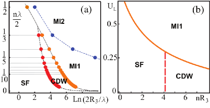
7.1.2 Bosonic gases in a deep optical lattice: extended Bose-Hubbard models
As discussed in the previous section, when all energy scales involved in the system dynamics are much smaller that the lattice bandwidth, both bosonic and fermionic gases are properly described in the context of Hubbard-like models. In the bosonic, single species case, the resulting extended Bose Hubbard Hamiltonian (EBHH)
| (110) |
contains kinetic energy (), local () and dipolar () interaction terms. The corresponding phase diagram has been studied in the grand-canonical ensemble in Ref. 262, where a Devil’s staircase structure has been shown to appear both in the hard-core (e.g., infinitely-large ) and soft-core (e.g., finite ) limits. Moreover, close to rational fillings, supersolid behavior has been suggested via both numerical and analytical methods, in particular close to the half-filled case, for both nearest-neighbor263, 264 and dipolar interactions265, whereas low and incommensurate filling fraction are still described by TLLs with both CDW and SF dominant orders266
Hidden order. In the special case of unit filling, that is, when the number of particles is equal to the number of lattice sites, an additional instability may occur. When dipolar and local interactions are much larger than the hopping rate , the competition between and gives rise to two different states of matter: a Mott insulator phase when , where double occupancies are suppressed, and a density wave (DW) when , where particles rearrange in a periodic structure in order to minimize the non-local repulsion (see Fig. 38). While these phases are separated by a first order phase transition line at strong coupling, in the intermediate interaction regime it has been shown that an additional state of matter, the so called Haldane insulator (HI), can emerge between the two 267. The HI is gapped and characterized in real space by a non-regular density pattern, where doubly occupied and empty sites are spatially separated by strings of singly occupied sites of uneven length (see the corresponding cartoon in Fig. 38). The occurrence of such magnetic-like order (between two doubly occupied sites there is always one and only one empty site) together with positional disorder (the length of the strings is not constant) is encoded into a string order parameter:
| (111) |
which approaches a constant value at large distances, ; here . In addition, the density wave order parameter, , which is constant in the DW phase, decays exponentially in the HI. Numerical simulations based on the density-matrix-renormalization-group (DMRG)268, 269 algorithm have quantitatively determined how this phase persists up to relatively large values of the interaction strength close to the line 267. In such a regime, where local occupations with are strongly suppressed, the bosonic Hamiltonian can be mapped into a spin-1 problem where the spin component along the -direction satisfies , and the and terms play the role of spin-exchange, dipolar interaction along the -axis and on-site anisotropy. The system thus resemble the so called Heisenberg model with single ion-anisotropy, or model, the only qualitative difference being the presence of a full dipolar tail instead of nearest-neighbor interaction, establishing a strong connection between the HI and the Haldane phase extensively studied in the context of magnetic systems 270, 271. An exact correspondence between bosonic and spin problem can be obtained in case of strong three-body losses 272, where the on-site Hilbert space is truncated up to doubly occupied states and the HI phase appears at smaller values of the dipolar interaction 273. The existence of such HI has been established even at higher integer fillings by mapping the problem to integer spin chains with spin 274.
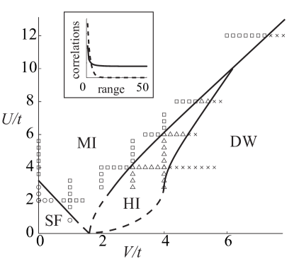
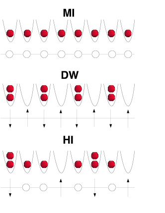
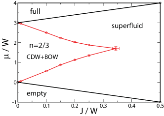
Three-body interactions. Additional interesting states of matter can be found in 1D version of Hamiltonians already treated in 2D in the previous section. As an example,it has been shown hot to engineer three-body interactions with polar molecules, leading to the effective Hamiltonian in Eq. (90). In 1D, the three-body term is responsible for the stabilization of an insulating phase at filling , which is driven by the fact that, above a certain ratio of , particles will minimize their potential energy by sitting in a periodic patter at the expenses of the kinetic one. Such phase transition belongs to the same universality class of the pinning one described in the shallow lattice case, and the critical value of the TLL parameter at the tip of the lobe is obtained from general considerations 222. The addition of a weak nearest neighbor repulsion can also stabilize a insulating state at filling when ; remarkably, the further addition of a next-nearest neighbor repulsion induces a competition between density wave and bond order wave, as the BOW phase broadens thanks to the three-body repulsion with respect to the case 275.
7.2 Two-species mixtures
The high degree of control over internal states of ultracold dipolar gases276 has opened the way towards the theoretical investigation of multispecies Hubbard-like models with additional dipolar interactions. While such specific models were not considered in standard condensed matter literature, Hamiltonians with nearest-neighbor interactions (which is, in many respects, similar to a dipolar one close to half-filling) such as the extended Hubbard model 245 have been shown to present a richer plethora of phases with respect to system with contact interactions only. The theoretical advantage of multispecies 1D systems with long-range interactions stems from the fact that one can understand their basic physical properties employing the same low-energy formalism used for models with contact interactions only245, 246. In the following, we will present an overview of theoretical results on two-species models with dipolar interactions, with both Fermionic and Fermi-Bose statistics.
7.2.1 Fermi-Fermi mixtures
Contrary to their two-dimensional counterparts, fermionic dipolar mixtures in 1D may be theoretically investigated with the same accuracy as bosonic ones. Defining as the creation/annihilation operators at the site of the species (we take here ), Fermi-Fermi mixtures in a deep optical lattice are usually described by the following Hamiltonian:
| (112) |
where the first two terms are hopping and on-site interaction, the third one is a species-dependent chemical potential, and the last one represent the dipolar contribution. When dealing with strong onsite two-body losses, the effective Hamiltonian has to be projected onto a constrained Hilbert space without double occupancies:
| (113) |
where . Such a picture, which reduces the on-site Hilbert space to just three states, is connected with the spin-1 chains (once is defined) already discussed in the context of the Haldane insulator phase for single species dipolar bosons; however, differently with respect to spin models, the key conserved quantity is , as can be inferred by performing a rigorous spin mapping 277. The phase diagram of Eq. (113) has been investigated at the mean field level and via numerical simulations based on the infinite time-evolving block decimation (iTEBD) 278 algorithm in Ref. 277 considering equal chemical potentials and intraspecies interactions, , and varying the interspecies one . This setup can be realized by, e.g., applying a pair of ac microwave fields close to the resonance of both internal states277. In the repulsive case, , the ground state is expected to show a dilute antiferromagnetic order of the form , where, between molecules of the same species, there is always one and only one molecule of the other species, in addition to two strings of empty sites. Such configurations display long-range order in the string correlation function
| (114) |
and can be distinguished into two different cases: when , all sites are occupied, and the ground state is an antiferromagnetic insulator (AFM); otherwise, the string order is dilute, the ground state is compressible and the so called Haldane liquid (HL) phase is stabilized. The mean field phase diagram presenting such competition is shown in Fig. 40, and has been supported by numerical iTEBD results, which show how, while both the AFM and the HL have long-range order in , other quantities such as standard spin-spin correlation functions have remarkably different behaviors 277, and in the HL phase may be qualitatively described by mapping the low-energy physics to a spinless TLL.


Using a combination of both DC and microwave external fields, as discussed in Sec. 8, it is also possible to engineer -like Hamiltonian with dipolar spin-exchange interactions, as described by the Hamiltonian:
| (115) |
where and . A complete investigation of the phase diagram of Eq. (115) is still lacking; nevertheless, the special case with , one of the simplest experimental realization, has been numerically investigated in Ref. 227 by means of DMRG calculations; in this case, the main difference with respect to the standard model resides in the long-range nature of the spin-exchange interactions, which are limited nearest-neighbor in the itself. At small values of , the ground state is a spin-density wave (SDW) at all densities, resembling the ground state physics of the strongly repulsive Hubbard model 245. Then, increasing , one enters first a region of singlet superfluidity (SS) with a finite spin gap (SG), and finally phase separation. In the SS region, inter-particle attraction is encoded into the TLL parameter of the density (or charge 245) sector . The main difference with the phase diagram of the model, which is reported in the upper panel of Fig. 41, is the presence of a larger gapped region; besides, the absence of a superfluid region with no spin gap (denoted as TS/SS) cannot be completely ruled out, as the broad blue region may indeed present such instability.

The realization of the model with polar molecules presents two main advantages for the purpose of exploring the physics of the model with ultracold gases: first, the accessible regions are not limited to small exchange couplings , and second the spin gap in the superfluid region is twice larger, making such phase more stable against thermal fluctuations 227.
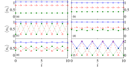
7.2.2 Bose-Fermi mixtures
Multispecies gases with different statistics, that is Bose-Fermi (BF) mixtures, have been the subject of numerous theoretical and experimental efforts in the field of cold atoms, and are currently being investigated even in presence of dipolar interactions. In 1D, the effective Hamiltonian of such systems when confined in a deep optical lattice is:
| (116) | |||||
where are creation operators obeying bosonic/fermionic statistics with respectively, the first line contains both hopping and chemical potential terms and the last two lines onsite and off-site interactions. The insulating instabilities of this Hamiltonian occurring close to half filling have been investigated in Ref. 279 by means of numerical simulations based on the iTEBD algorithm by truncating the dipolar interactions up to nearest-neighbors and considering several combination in the broad parameter space of . In addition to gapless liquid and density-wave phases (a BF liquid, Fig. 42 (a), and a BF density wave, Fig. 42 (e)), BF Mott phases with and without density oscillations are present (a BF Mott insulator, Fig. 42 (b), and a BF Mott density wave, Fig. 42 (d)). Finally, in the special case of half filling for both species, a BF solid, an incompressible phase with an alternating density pattern (Fig. 42 (c) and (f)), is also stable in the strongly interacting regime . Such phase displays true-long range order and, differently from the Néel antiferromagnetic case realized with purely contact interactions, is stable even when considering equal tunneling rates ; moreover, it displays very different melting processes as the interaction are increased depending on the relative value of 279.
7.3 Quasi-1D physics: coupling between tubes
The long-range nature of dipolar interactions is well suited to create hybrid systems with purely 1D dynamics but 2D interactions, such as arrays of coupled tubes divided by very deep optical lattices preventing inter-tube tunneling together with a proper tuning of the external DC electric fields in order to manipulate the inter-tube interaction, as seen in Sec.2. Such systems establish a deep connection between the physics of several condensed matter systems such as, e.g., spin compounds 245 and ultracold dipolar gases which cannot be explored with contact interactions only. In the following, we first present recent results on the two-tube case, or two-leg ladder, and then consider the 2D limit where a large number of tubes, a planar array, is taken into account.
7.3.1 Two-leg ladders
Dipolar ladders allow to investigate rich physical phenomena by matching the advantages of reduced loss rates typical of 1D confinement with the possibility of considering multispecies physics, where the physical species index is represented by the wire one 222The case of multispecies gases confined in quasi-1D geometries, which allows to treat problems with even more degrees of freedom, has attracted little attention so far.. In this respect, the special case of two-coupled tubes has been widely investigated. The effective Hamiltonian of such systems, in case an optical lattice in the tube direction is applied, is very similar to a two-species gas,
| (117) | |||||
| (118) |
with the remarkable difference that here the anisotropic nature of the dipole-dipole interaction plays a prominent role. Here, is the wire-index, and the specific shape of depends on both the inter-wire distance and the angle between the dipole moments and the plane the ladder lies on. Moreover, for bosonic particles, an additional term denotes the on-site interaction.
Bosonic ladders. As a first step, it is worth considering if and how phases typical of 1D setups such as Mott insulators, superfluids and Haldane insulators are changed in ladder geometries. In case of interwire attraction, both MI and SF phases appear in the limit of small ()and large () intrawire tunneling respectively, and a pair superfluid phase (PSF), that is, a superfluid ground state of composite particles made of one boson on each tube, is stabilized at intermediate values of 280. The Mott lobes close to the PSF phase have remarkably different excitations, that is, particle-hole are substituted by creation/annihilation of composite particles, further increasing the re-entrant shape of the Mott lobes, as can be seen in Fig. 43. The evolution of the HI phase in ladder setups in indeed more tantalizing, as in the case of spin-1 chains it has been shown that the string order of the Haldane phase is unstable towards weak antiferromagnetic interchain exchange perturbations 281. In the case of bosonics coupled tubes, combining TLL theory with renormalization group arguments, it has been shown 282 that, while a small intertube repulsion changes only quantitatively the shape of the phase diagram, interchain tunneling terms of the type:
| (119) |
open an additional gapless, superfluid phase between the two: a schematic view of such changes is presented in Fig. 44, and has been confirmed numerically via DMRG simulations 282, 283.


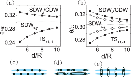
Fermionic ladders. Fermionic ladders present more instabilities with respect to the single tube, single species case. In absence of a lattice, the weak-coupling phase diagram has been investigated using the bosonization formalism 247, 246 in various setups 284, 285. In case of short range interwire repulsion, the interplay between the longitudinal confinement length , the interwire distance and the angle (see Fig. 2) is responsible for the stabilization of three main phases. In case of intrawire attraction, , pairing on the single wire is favored, giving rise to a triplet superfluid phase (TS); in the opposite case of intrawire repulsion, , a spin density wave with alternating order (SDWz) appears, while in the intermediate regime the dominant order is an in-plane spin-density wave (SDWx,y) 284. In the case of a deep lattice, Eq. (118) becomes an extension of the so called anisotropic extended Hubbard model (AEHM) 286 with both large anisotropy and long-range, dipolar terms; while all the previous phases are expected to appear in the low-density limit, the possibility of tuning independently inter- and intra-wire repulsion, making the former stronger than the latter, leads to a spontaneous breaking of the symmetry associated with the ladder geometry, stabilizing a fully polarized ground state where all particles stay on the same tube to minimize the inter-tube repulsion. Moreover, the addition of inter-wire tunneling terms (Eq. (119)) may stabilize additional phases 284.
When inter-wire interactions are turned attractive, a different physical picture arises depending on the population ratio between the wires, . When , pairing between the tubes is always favored, and the system behaves like a quantum liquid of composite bosonic particles made of one boson per wire; such a liquid can be both a superfluid (that is, a PSF), or a CDW depending on both the interwire distance and dipole strength 285. If a shallow optical lattice commensurate with the particle density is introduced along the tube direction, that is its lattice wavelength satisfies , the system can undergo a BKT transition to a composite crystal as a function of the lattice depth, in analogy with what happens in the single tube bosonic case (see Sec. 7.1.1): in a grand canonical ensemble, this picture evolves establishing a Luttinger staircase of dimer crystals 285. In the deep lattice case, these predictions have been checked by means of DMRG simulations.
Imbalanced ladders. A completely different phenomenon occurs in presence of a density imbalance between the tubes. For interwire distances larger than the inverse particle density, the long-range nature of the dipolar interaction creates an effective fixed range interwire attraction, thus favoring pairing not only between two, but also between many particles. In the special case of commensurate densities between the wires, , a gas of composite particles, or multimers, composed by particles in the first (second) wire respectively can be stabilized for sufficiently low densities 285. Such a multimer liquid picture has a description in terms of low-energy field theory 287, and allows to study generalized pairing mechanism beyond two-particle ones. In the special case of , the stability of trimer liquids has been confirmed numerically for sufficiently large tunneling and dipole imbalance between the tubes. When also a trapping potential and a non-ideal population ratio is considered, such trimer liquids (which are not stable in homogeneous setups with unmatched densities) appear in the center of the system, and are surrounded by both dimer liquids or singles species ones depending on the population ration, forming a pancake-like structure of composite liquids (see Fig. 46) as shown in recent DMRG simulations 285.
The possibility of further tuning the numerous parameters of the ladder Hamiltonian Eq. (118) may indeed allow to identify additional exotic state of matter, as the complete phase diagram of these system is still largely unexplored. Moreover, before turning our attention to systems composed by a large number of tubes, it is worth noticing that ladder systems with more than two tubes and mixtures in quasi-1D geometries are in principle good candidates to study new model Hamiltonians in connection to many-body problems with many degrees of freedom.
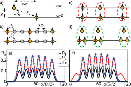
7.3.2 Planar array of tubes
Planar arrays of tubes of dipolar gases constitute a hybrid setup where one can investigate 2D states of matter with physical properties typical of 1D systems such as, e.g., quasi long range order of correlation functions. Even in this case, the effective Hamiltonian:
has many controllable parameters: here, are creation/annihilation operator on the tube (sums over Greek indices denote sums over the tube index, while Latin indices denote particles along each tube), , the first term represents the kinetic energy over each tube and the second one the dipolar interactions, which depend on both strength and orientation of the dipole moments. In the zero-density limit, where only one bosonic particle per wire is considered and inter-wire interaction are attractive, a quantum rough chain forms with the off-diagonal long range order in the -body correlation function, where is the number of wires 288.
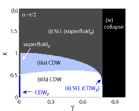
In the finite density regime, the many body physics displays very different effects. In the bosonic case with intrawire dipolar repulsion, the competition between local interactions and long-range ones is encoded into a dimensionless parameter , where and are the sound velocity and the TLL parameter of a single tube, is the strength of the dipolar interactions and the intertube spacing. By varying both and , one can span a broad parameter region with respect to the dipolar interaction, the density of particles and the -wave scattering length 289. In addition to a series of density wave states driven by the strong dipolar repulsion, which may lead to both a stripe and checkerboard order depending on the relative strength between inter- and intra-tube repulsion, a gapless phase (denoted as (i) in Fig. 47) with dominant superfluid correlations along the tubes is present for large values of (that is, for weak intratube interactions) 289. Such a phase, which despite being effectively two-dimensional still preserves an algebraic decay of correlation functions typical of the quasi-long range order of 1D systems, is known as sliding Luttinger liquid (SLL), and has been investigated even in several fermionic models related to stripe physics and high-Tc superconductivity 290. Moreover, the SLL phase may also have dominant density-density correlation along the tube in a tiny region at intermediate (denoted as (ii)). In the strongly interacting regime, a collapsed regime take place, whose precise shape depends on the sign of the intertube interactions. The complete phase diagram for a fixed value of the angle is shown in Fig. 47.
The planar array of fermionic dipoles displays a different phase diagram, albeit some features such as the density wave patterns emerge independently on the statistics. The phase diagram of this system as a function of the angles and (see Fig. 2) have been derived in the framework of a generalized TLL theory 291 by comparing the long-distance decay of several correlation functions, as reported in Fig. 48. When both inter- and intra-tube interactions are strongly repulsive, the ground state exhibits CDW (checkerboard) order, similarly to the bosonic case. Close to the magic angle , where the intrawire interaction turns from repulsive to attractive, an intertube superfluid (-SF) phase together with a density wave with broken particle number conservation along the tubes (or gauge-phase density wave, GPDW) are present. Finally, for attractive intratube interactions, a -wave superfluid (-SF) is the precursor of an unstable phase toward intratube collapse.
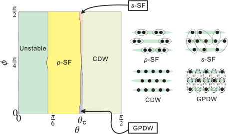
8 Conclusions and outlook
The many-body systems discussed in this review are examples of the variety of physical properties which originate from the anisotropy and long-range character of dipole-dipole interactions, in combination with their tunability with external fields. In many physical situations quantum dipolar gases behave qualitatively different when compared to atomic gases with short-range van der Waals interactions, and provide us with a large number of novel quantum systems with unique physical properties. Understanding the many-body behavior of these systems is a very interesting and challenging problem with several potentially significant consequences for fundamental science and practical applications.
In the present review we have focused on dipolar quantum gases represented by polar molecules in the rovibrational ground state. An alternative realization of a dipolar quantum gas, although in a completely different regime, is a gas of laser excited Rydberg atoms 292 or molecules 293, 294. Highly excited Rydberg atoms and molecules interact via remarkably strong electric dipole moments or Van der Waals interactions. This leads to the phenomenon of a dipole blockade and formation of superatoms where within a given blockade radius only a single Rydberg atom can be excited, and, for example, crystals of these superatoms can be formed 292. In view of the finite life time of Rydberg states these many body phases will only exist for a comparatively short time in the so-called frozen gas regime where there is no atomic motion. However, as discussed in Ref. 150, the large Rydberg dipoles can also be admixed weakly to the ground state by off-resonant laser excitation which provides a situation loosely reminiscent of the polar molecule case, although decoherence due to spontaneous emission remains always an issue.
Finally, we remark that the tools for manipulating interactions in dipolar systems, as described in the present review, also provide promising ingredients for controlled entanglement between polar molecules, and thus possible new scenarios for quantum computing 295, 296, 297. Loading exactly one atom or molecules per lattice site via a Mott insulator transition in an optical lattice provides us with an array of qubits. In the case of polar molecules, the qubits can he represented by long-lived rotational or spin degrees of freedom. Single site addressing, as developed in Refs. 6, 7 for atoms, allows to both manipulate as well as read out the single qubit. Entanglement of qubits can be achieved via the strong and long range dipolar interactions between molecules 295, 296, 297, or in the atomic case via dipolar Rydberg interactions292.
9 Acknowledgements
We would like to thank I. Bloch, D. Blume, J. Bohn, H. P. Büchler, L. D. Carr, N. R. Cooper, R. Côté, D. DeMille, E. Demler, J. Doyle, F. Ferlaino A. Gorshkov, M. Lewenstein, M. Lukin, D. Jin, P. Julienne, R. Krems, B. Lev, G. Mejier, H. C. Nägerl, D. Petrov, T. Pfau, G. Quéméner, L. Santos, G. Shlyapnikov, J. Ye, S. Yelin, D.-W. Wang and M. Weidemüller for many interesting discussion on the topics treated in this review. Work supported by the Austrian Science Fund, EU grants AQUTE, COHERENCE and NAME-QUAM, and by MURI, AFOSR, ISIS, EOARD, IPCMS and the RTRA Foundation.
10 Biographies


References
- Metcalf and van der Straten 1999 Metcalf, H. J.; van der Straten, P. Laser Cooling and Trapping; Springer-Verlag, New York, 1999
- Chin et al. 2010 Chin, C.; Grimm, R.; Julienne, P.; Tiesinga, E. Rev. Mod. Phys. 2010, 82, 1225–1286
- Bloch et al. 2008 Bloch, I.; Dalibard, J.; Zwerger, W. Rev. Mod. Phys. 2008, 80, 885
- Bloch 2005 Bloch, I. Nature Physics 2005, 1, 23
- Greiner and Fölling 2008 Greiner, M.; Fölling, S. Nature 2008, 453, 736
- Bakr et al. 2009 Bakr, W. S.; Gillen, J. I.; Peng, A.; Fölling, S.; Greiner, M. Nature 2009, 462, 74
- Sherson et al. 2010 Sherson, J.; Weitenberg, C.; Endres, M.; Cheneau, M.; Bloch, I.; Kuhr, S. Nature 2010,
- Edited by M. Inguscio and Salomon 2008 Edited by M. Inguscio, W. K.; Salomon, C. Proceedings of the International School of Physics Enrico Fermi, Course CLXIV, Varenna, 20-30 June 2006; IOP Press, Amsterdam, 2008
- Hadzibabic et al. 2006 Hadzibabic, Z.; Kruger, P.; Cheneau, M.; Battelier, B.; Dalibard, J. Nature 2006, 441, 1118–1121
- Griesmaier et al. 2005 Griesmaier, A.; Werner, J.; Hensler, S.; Stuhler, J.; Pfau, T. Phys. Rev. Lett. 2005, 94, 160401
- Stuhler et al. 2005 Stuhler, J.; Griesmaier, A.; Koch, T.; Fattori, M.; Pfau, T.; Giovanazzi, S.; Pedri, P.; Santos, L. Physical review letters 2005, 95, 150406
- Fattori et al. 2006 Fattori, M.; Koch, T.; Goetz, S.; Griesmaier, A.; Hensler, S.; Stuhler, J.; Pfau, T. Nat Phys 2006, 2, 765–768
- Griesmaier et al. 2006 Griesmaier, A.; Stuhler, J.; Koch, T.; Fattori, M.; Pfau, T.; Giovanazzi, S. Phys. Rev. Lett. 2006, 97, 250402
- Lahaye et al. 2007 Lahaye, T.; Koch, T.; Fröhlich, B.; Fattori, M.; Metz, J.; Griesmaier, A.; Giovanazzi, S.; Pfau, T. Nature 2007, 448, 672–675
- Koch et al. 2008 Koch, T.; Lahaye, T.; Metz, J.; Fröhlich, B.; Griesmaier, A.; Pfau, T. Nat Phys 2008, 4, 218–222
- Lahaye et al. 2008 Lahaye, T.; Metz, J.; Fröhlich, B.; Koch, T.; Meister, M.; Griesmaier, A.; Pfau, T.; Saito, H.; Kawaguchi, Y.; Ueda, M. Phys. Rev. Lett. 2008, 101, 080401
- Aikawa et al. 2012 Aikawa, K.; Frisch, A.; Mark, M.; Baier, S.; Rietzler, A.; Grimm, R.; Ferlaino, F. arXiv.1204.1725 2012,
- Lu et al. 2011 Lu, M.; Burdick, N. Q.; Youn, S. H.; Lev, B. L. Phys. Rev. Lett. 2011, 107, 190401
- Lu et al. 2012 Lu, M.; Burdick, N. Q.; Lev, B. L. arXiv.1202.4444v3 2012,
- Weinstein et al. 1998 Weinstein, J. D.; DeCarvalho, R.; Guillet, T.; Friedrich, B.; Doyle, J. M. Nature 1998, 395, 148–150
- Doyle and Friedrich 1999 Doyle, J. M.; Friedrich, B. Nature 1999, 401, 749–751
- Bethlem et al. 1999 Bethlem, H. L.; Berden, G.; Meijer, G. Phys. Rev. Lett. 1999, 83, 1558–1561
- Bethlem et al. 2000 Bethlem, H. L.; Berden, G.; van Roij, A. J. A.; Crompvoets, F. M. H.; Meijer, G. Phys. Rev. Lett. 2000, 84, 5744–5747
- Bethlem et al. 2000 Bethlem, H. L.; Berden, G.; Crompvoets, F. M. H.; Jongma, R. T.; van Roij, A. J. A.; Meijer, G. Nature 2000, 406, 491–495
- Bethlem et al. 2002 Bethlem, H. L.; Crompvoets, F. M. H.; Jongma, R. T.; van de Meerakker, S. Y. T.; Meijer, G. Phys. Rev. A 2002, 65, 053416
- PM7 2004 Special Issue on “Ultracold Polar Molecules: Formation and Collisions”; edited by J. Doyle, B. Friedrich, R.V. Krems and Masnou-Seeuws, F., Eur. Phys. J. D, 2004; Vol. 31
- van de Meerakker et al. 2005 van de Meerakker, S. Y. T.; Smeets, P. H. M.; Vanhaecke, N.; Jongma, R. T.; Meijer, G. Phys. Rev. Lett. 2005, 94, 023004
- Bochinski et al. 2004 Bochinski, J. R.; Hudson, E. R.; Lewandowski, H. J.; Ye, J. Phys. Rev. A 2004, 70, 043410
- Wang et al. 2004 Wang, D.; Qi, J.; Stone, M.; Nikolayeva, O.; Hattaway, B.; Gensemer, S.; Wang, H.; Zemke, W.; Gould, P.; Eyler, E.; Stwalley, W. Eur. Phys. J. D 2004, 31, 165
- Egorov et al. 2004 Egorov, D.; Campbell, W. C.; Friedrich, B.; Maxwell, S. E.; Tsikata, E.; van Buuren, L. D.; Doyle, J. M. Eur. Phys. J. D - Atomic, Molecular, Optical and Plasma Physics 2004, 31, 307–311
- Sage et al. 2005 Sage, J. M.; Sainis, S.; Bergeman, T.; DeMille, D. Phys. Rev. Lett. 2005, 94, 203001
- Baranov 2008 Baranov, M. Physics Reports 2008, 464, 71 – 111
- Carr et al. 2009 Carr, L. D.; DeMille, D.; Krems, R. V.; Ye, J. New J. Phys. 2009, 11, 055049
- Lahaye et al. 2009 Lahaye, T.; Menotti, C.; Santos, L.; Lewenstein, M.; Pfau, T. Rep. Prog. Phys. 2009, 72, 126401
- Krems et al. 2009 Krems, R. V.; Stwalley, W. C.; Friedrich, B. Cold Molecules: Theory, Experiment, Applications; CRC Press, 2009
- Trefzger et al. 2011 Trefzger, C.; Menotti, C.; Capogrosso-Sansone, B.; Lewenstein, M. J. Phys. B: At. Mol. Opt. Phys. 2011, 44, 193001
- Müller et al. 2011 Müller, S.; Billy, J.; Henn, E. A. L.; Kadau, H.; Griesmaier, A.; Jona-Lasinio, M.; Santos, L.; Pfau, T. 2011, arXiv:1105.5015
- Marinescu and You 1998 Marinescu, M.; You, L. Phys. Rev. Lett. 1998, 81, 4596–4599
- Deb and You 2001 Deb, B.; You, L. Phys. Rev. A 2001, 64, 022717
- Yi and You 2000 Yi, S.; You, L. Phys. Rev. A 2000, 61, 041604
- Ronen et al. 2006 Ronen, S.; Bortolotti, D. C. E.; Blume, D.; Bohn, J. L. Phys. Rev. A 2006, 74, 033611
- Derevianko 2003 Derevianko, A. Phys. Rev. A 2003, 67, 033607
- Derevianko 2005 Derevianko, A. Phys. Rev. A 2005, 72, 039901
- Bortolotti et al. 2006 Bortolotti, D. C. E.; Ronen, S.; Bohn, J. L.; Blume, D. Phys. Rev. Lett. 2006, 97, 160402
- Giovanazzi et al. 2002 Giovanazzi, S.; Görlitz, A.; Pfau, T. Phys. Rev. Lett. 2002, 89, 130401
- Mehring 1983 Mehring, M. Principles of High Resolution NMR in Solids; Springer, Berlin, 1983
- Zuchowski and Hutson 2010 Zuchowski, P. S.; Hutson, J. M. Phys. Rev. A 2010, 81, 060703
- Idziaszek and Julienne 2010 Idziaszek, Z.; Julienne, P. S. Phys. Rev. Lett. 2010, 104, 113202
- Idziaszek et al. 2010 Idziaszek, Z.; Quemener, G.; Bohn, J. L.; Julienne, P. S. Phys. Rev. A 2010, 020703 (R)
- Ni et al. 2010 Ni, K.-K.; Ospelkaus, S.; Wang, D.; Quemener, G.; Neyenhuis, B.; de Miranda, M. H. G.; Bohn, J. L.; Ye, J.; Jin, D. S. Nature 2010, 464, 1324
- de Miranda et al. 2011 de Miranda, M. H. G.; Chotia, A.; Neyenhuis, B.; Wang, D.; Quéméner, G.; Ospelkaus, S.; Bohn, J. L.; Ye, J.; Jin, D. S. Nature Physics 2011, 7, 502
- Ticknor 2010 Ticknor, C. Phys. Rev. A 2010, 81, 042708
- Quéméner and Bohn 2010 Quéméner, G.; Bohn, J. L. Phys. Rev. A 2010, 81, 060701 (R)
- Petrov and Shlyapnikov 2001 Petrov, D.; Shlyapnikov, G. Phys. Rev. A 2001, 64, 012706
- Li et al. 2008 Li, Z.; Alyabyshev, S. V.; Krems, R. V. Phys. Rev. Lett. 2008, 100, 073202
- Li and Krems 2009 Li, Z.; Krems, R. V. Phys. Rev. A 2009, 79, 050701
- Micheli et al. 2007 Micheli, A.; Pupillo, G.; Büchler, H. P.; Zoller, P. Phys. Rev. A 2007, 76, 043604
- Gribakin and Flambaum 1993 Gribakin, G. F.; Flambaum, V. V. Phys. Rev. A 1993, 48, 546
- Julienne 2009 Julienne, P. S. Faraday Discuss. 2009, 142, 361
- Micheli et al. 2010 Micheli, A.; Idziaszek, Z.; Pupillo, G.; Baranov, M. A.; Zoller, P.; Julienne, P. S. Phys. Rev. Lett. 2010, 105, 073202
- Julienne et al. 2011 Julienne, P. S.; Hanna, T. M.; Idziaszek, Z. Phys. Chem. Chem. Phys. 2011,
- Coleman 1977 Coleman, S. Phys. Rev. D 1977, 15, 2929–2936
- Quéméner and Bohn 2010 Quéméner, G.; Bohn, J. L. Phys. Rev. A 2010, 81, 022702
- Buechler et al. 2007 Buechler, H. P.; Demler, E.; Lukin, M.; Micheli, a.; Prokof’ev, N.; Pupillo, G.; Zoller, P.; Büchler, H. P.; Prokof’ev, N. Phys. Rev. Lett. 2007, 98, 60404
- Zilio et al. 1996 Zilio, S. C.; Marcassa, L.; Muniz, S.; Horowicz, R.; Bagnato, V.; Napolitano, R.; Weiner, J.; Julienne, P. S. Phys. Rev. Lett. 1996, 76, 2033–2036
- Napolitano et al. 1997 Napolitano, R.; Weiner, J.; Julienne, P. S. Phys. Rev. A 1997, 55, 1191–1207
- Weiner et al. 1999 Weiner, J.; Bagnato, V. S.; Zilio, S.; Julienne, P. S. Rev. Mod. Phys. 1999, 71, 1–85
- Gorshkov et al. 2008 Gorshkov, A. V.; Rabl, P.; Pupillo, G.; Micheli, A.; Zoller, P.; Lukin, M. D.; Büchler, H. P. Phys. Rev. Lett. 2008, 101, 073201, Phys. Rev
- Aldegunde et al. 2009 Aldegunde, J.; Ran, H.; Hutson, J. M. Phys. Rev. A 2009, 80, 043410
- Ran et al. 2010 Ran, H.; Aldegunde, J.; Hutson, J. M. New J. Phys. 2010, 12, 043015
- Ticknor and Bohn 2005 Ticknor, C.; Bohn, J. L. Phys. Rev. A 2005, 72, 032717
- Dalfovo et al. 1999 Dalfovo, F.; Giorgini, S.; Pitaevskii, L. P.; Stringari, S. Rev. Mod. Phys. 1999, 71, 463–512
- Yi and You 2001 Yi, S.; You, L. Phys. Rev. A 2001, 63, 053607
- Santos et al. 2000 Santos, L.; Shlyapnikov, G. V.; Zoller, P.; Lewenstein, M. Phys. Rev. Lett. 2000, 85, 1791–1794
- Lushnikov 2002 Lushnikov, P. M. Phys. Rev. A 2002, 66, 051601
- Santos et al. 2002 Santos, L.; Shlyapnikov, G. V.; Zoller, P.; Lewenstein, M. Phys. Rev. Lett. 2002, 88, 139904
- Dutta and Meystre 2007 Dutta, O.; Meystre, P. Phys. Rev. A 2007, 75, 053604
- Eberlein et al. 2005 Eberlein, C.; Giovanazzi, S.; O’Dell, D. H. J. Phys. Rev. A 2005, 71, 033618
- Ronen et al. 2007 Ronen, S.; Bortolotti, D. C. E.; Bohn, J. L. Phys. Rev. Lett. 2007, 98, 030406
- Góral et al. 2000 Góral, K.; Rza¸żewski, K.; Pfau, T. Phys. Rev. A 2000, 61, 051601
- Martikainen et al. 2001 Martikainen, J.-P.; Mackie, M.; Suominen, K.-A. Phys. Rev. A 2001, 64, 037601
- Santos et al. 2003 Santos, L.; Shlyapnikov, G. V.; Lewenstein, M. Phys. Rev. Lett. 2003, 90, 250403
- Ruprecht et al. 1996 Ruprecht, P. A.; Edwards, M.; Burnett, K.; Clark, C. W. Phys. Rev. A 1996, 54, 4178–4187
- Góral and Santos 2002 Góral, K.; Santos, L. Phys. Rev. A 2002, 66, 023613
- O’Dell et al. 2004 O’Dell, D. H. J.; Giovanazzi, S.; Eberlein, C. Phys. Rev. Lett. 2004, 92, 250401
- Baranov et al. 2002 Baranov, M. A.; Dobrek, Ł.; Góral, K.; Santos, L.; Lewenstein, M. Physica Scripta 2002, 2002, 74
- Fischer 2006 Fischer, U. R. Phys. Rev. A 2006, 73, 031602
- Stringari 1998 Stringari, S. Phys. Rev. A 1998, 58, 2385–2388
- Landau and Lifshitz 1981 Landau, L. D.; Lifshitz, L. M. Quantum Mechanics {Non-Relativistic} Theory, Third Edition: Volume 3; Butterworth-Heinemann, 1981
- Lifshitz and Pitaevskii 1980 Lifshitz, E.; Pitaevskii, L. Statistical Physics, Part 2; Butterworth-Heinemann, 1980
- Pomeranchuk 1958 Pomeranchuk, I. Sov. Phys. JETP 1958, 8, 361
- Miyakawa et al. 2008 Miyakawa, T.; Sogo, T.; Pu, H. Phys. Rev. A 2008, 77, 061603
- Sogo et al. 2008 Sogo, T.; He, L.; Miyakawa, T.; Yi, S.; Pu, H. New J. Phys. 2008, 11, 055017
- Ronen and Bohn 2010 Ronen, S.; Bohn, J. L. Phys. Rev. A 2010, 81, 033601
- Chan et al. 2010 Chan, C.-K.; Wu, C.; Lee, W.-C.; Das Sarma, S. Phys. Rev. A 2010, 81, 023602
- Kestner and Das Sarma 2010 Kestner, J. P.; Das Sarma, S. Phys. Rev. A 2010, 82, 033608
- Sieberer and Baranov 2011 Sieberer, L. M.; Baranov, M. A. Phys. Rev. A 2011, 84, 063633
- Lu and Shlyapnikov 2012 Lu, Z.-K.; Shlyapnikov, G. V. Phys. Rev. A 2012, 85, 023614
- You and Marinescu 1999 You, L.; Marinescu, M. Phys. Rev. A 1999, 60, 2324–2329
- Stoof and Houbiers 1999 Stoof, H.; Houbiers, M. 1999, arXiv:9808171
- Baranov et al. 2002 Baranov, M. A.; Mar’enko, M. S.; Rychkov, V. S.; Shlyapnikov, G. V. Phys. Rev. A 2002, 66, 013606
- J. Bardeen and Schrieffer 1957 J. Bardeen, L. C.; Schrieffer, J. Phys. Rev. 1957, 108, 1175
- Leggett 47 Leggett, A. J. Rev. Mod. Phys. 47, 1975, 331
- Gor’kov and Melik-Barkhudarov 1961 Gor’kov, L.; Melik-Barkhudarov, T. Sov. Phys. JETP 1961, 13, 1018
- Vollhardt and Wölfle 1990 Vollhardt, D.; Wölfle, P. The Superfluid Phases of Helium 3; Taylor and Francis, London, 1990
- Volovik and Gor’kov 1985 Volovik, G.; Gor’kov, L. Sov. Phys. JETP 1985, 61, 843
- Marchenko 1986 Marchenko, V. Sov. Phys. JETP 1986, 66, 331
- Sigrist and Ueda 1991 Sigrist, M.; Ueda, K. Rev. Mod. Phys. 1991, 63, 239–311
- Fisher et al. 1989 Fisher, R. A.; Kim, S.; Woodfield, B. F.; Phillips, N. E.; Taillefer, L.; Hasselbach, K.; Flouquet, J.; Giorgi, A. L.; Smith, J. L. Phys. Rev. Lett. 1989, 62, 1411–1414
- Baranov et al. 2004 Baranov, M. A.; Dobrek, Ł.; Lewenstein, M. New Journal of Physics 2004, 6, 198
- Baranov and Petrov 1998 Baranov, M. A.; Petrov, D. S. Phys. Rev. A 1998, 58, R801–R804
- Bruun et al. 1999 Bruun, G.; Castin, Y.; Dum, R.; Burnett, K. Eur. Phys. J. D 1999, 7, 433, 10.1007/s100530050587
- Viverit et al. 2004 Viverit, L.; Bruun, G. M.; Minguzzi, A.; Fazio, R. Phys. Rev. Lett. 2004, 93, 110406
- Shi et al. 2010 Shi, T.; Zhang, J.-N.; Sun, C.-P.; Yi, S. Phys. Rev. A 2010, 82, 033623
- Bruun and Taylor 2008 Bruun, G. M.; Taylor, E. Phys. Rev. Lett. 2008, 101, 245301
- Berezinskii 1972 Berezinskii, V. L. JETP 1972, 34, 610
- J. M. Kosterlitz 1973 J. M. Kosterlitz, T., D. J J. Phys. C. 1973, 6, 1181
- Kosterlitz 1974 Kosterlitz, J. J. Phys. C: Solid State Phys 1974, 7, 1046–1060
- Miyake 1983 Miyake, K. Prog. Theor. Phys. 1983, 69, 1794–1797
- Cooper and Shlyapnikov 2009 Cooper, N. R.; Shlyapnikov, G. V. Phys. Rev. Lett. 2009, 103, 155302
- Levinsen et al. 2011 Levinsen, J.; Cooper, N. R.; Shlyapnikov, G. V. Phys. Rev. A 2011, 84, 013603
- Volovik 1992 Volovik, G. Exotic Properties of Superfluid 3He; World Scientific, Singapore, 1992
- Read and Green 2000 Read, N.; Green, D. Phys. Rev. B 2000, 61, 10267–10297
- Stern 2008 Stern, A. Ann. Phys. 2008, 323, 204–249
- Nayak et al. 2008 Nayak, C.; Simon, S. H.; Stern, A.; Freedman, M.; Das Sarma, S. Rev. Mod. Phys. 2008, 80, 1083–1159
- Pikovski et al. 2010 Pikovski, A.; Klawunn, M.; Shlyapnikov, G. V.; Santos, L. Phys. Rev. Lett. 2010, 105, 215302
- Baranov et al. 2011 Baranov, M. A.; Micheli, A.; Ronen, S.; Zoller, P. Phys. Rev. A 2011, 83, 043602
- Klawunn et al. 2010 Klawunn, M.; Pikovski, A.; Santos, L. Phys. Rev. A 2010, 82, 044701
- Taylor 1972 Taylor, J. Scattering Theory; John Wiley and Sons, New York, 1972
- Zinner et al. 2012 Zinner, N. T.; Wunsch, B.; Pekker, D.; Wang, D.-W. Phys. Rev. A 2012, 85, 013603
- Góral et al. 2001 Góral, K.; Englert, B.-G.; Rza¸żewski, K. Phys. Rev. A 2001, 63, 033606
- Pines and P. 1966 Pines, D.; P., N. The Theory of Quantum Liquids; W.A. Benjamin, Inc., 1966
- Sun et al. 2010 Sun, K.; Wu, C.; Das Sarma, S. Phys. Rev. B 2010, 82, 075105
- Zinner and Bruun 2011 Zinner, N. T.; Bruun, G. M. Eur. Phys. J. D 2011, 65, 133–139
- Babadi and Demler 2011 Babadi, M.; Demler, E. Phys. Rev. B 2011, 84, 235124
- Wang et al. 2006 Wang, D.-W.; Lukin, M. D.; Demler, E. Phys. Rev. Lett. 2006, 97, 180413
- Klawunn et al. 2010 Klawunn, M.; Duhme, J.; Santos, L. Phys. Rev. A 2010, 81, 013604
- Volosniev et al. 2011 Volosniev, A. G.; Fedorov, D. V.; Jensen, A. S.; Zinner, N. T. 2011, arXiv.1109.4602
- Volosniev et al. 2011 Volosniev, A. G.; Armstrong, J. R.; Fedorov, D. V.; Jensen, A. S.; Zinner, N. T. 2011, arXiv.1112.2541
- Potter et al. 2010 Potter, A. C.; Berg, E.; Wang, D.-W.; Halperin, B. I.; Demler, E. Phys. Rev. Lett. 2010, 105, 220406
- Kalia and Vashishta 1981 Kalia, R. K.; Vashishta, P. J. Phys. C. 1981, 14, L643
- Bruun and Taylor 2008 Bruun, G. M.; Taylor, E. Phys. Rev. Lett. 2008, 101, 245301
- Wineland et al. 1998 Wineland, D.; Monroe, C.; Itano, W. M.; Leibfried, D.; King, B. E.; Meekhof, D. M. J.Res.Natl.Inst.Stand.Tech. 1998, 103, 259
- Filinov et al. 2010 Filinov, A.; Prokof’ev, N.; Bonitz, M. Phys. Rev. Lett. 2010, 105, 070401
- Boninsegni et al. 2006 Boninsegni, M.; Prokof’ev, N.; Svistunov, B. Phys. Rev. Lett. 2006, 96, 070601
- Astrakharchik et al. 2007 Astrakharchik, G.; Boronat, J.; Kurbakov, I.; Lozovik, Y. Phys. Rev. Lett. 2007, 98, 060405
- Mora et al. 2007 Mora, C.; Parcollet, O.; Waintal, X. Phys. Rev. B 2007, 76, 064511
- F. Mazzanti and Boronat 2009 F. Mazzanti, G. E. A., R. E. Zillich; Boronat, J. Phys. Rev. Lett. 2009, 102, 110405
- Hufnagl et al. 2011 Hufnagl, D.; Kaltseis, R.; Apaja, V.; Zillich, R. E. Phys. Rev. Lett. 2011, 107, 065303
- Pupillo et al. 2010 Pupillo, G.; Micheli, A.; Boninsegni, M.; Lesanovsky, I.; Zoller, P. Phys. Rev. Lett. 2010, 104, 223002
- Belousov and Lozovik 2000 Belousov, A. I.; Lozovik, Y. E. Eur. Phys. J. D 2000, 8, 251
- Yu. E. Lozovik and Willander 2004 Yu. E. Lozovik, S. Y. V.; Willander, M. JETP Letters 2004, 79, 473
- Ludwig et al. 2008 Ludwig, P.; Balzer, K.; Filinov, A.; Stolz, H.; Bonitz, M. New J. Phys. 2008, 10, 083031
- Bedanov and Peeters 1994 Bedanov, V. M.; Peeters, F. M. Phys. Rev. B 1994, 49, 2667
- Filinov et al. 2008 Filinov, A.; Böning, J.; Bonitz, M.; Lozovik, Y. Phys. Rev. B 2008, 77, 214527
- Pupillo et al. 2009 Pupillo, G.; Micheli, A.; Boninsegni, M.; Lesanovsky, I.; Zoller, P. arXiv:0904.2735 2009,
- J. Piyush and Boninsegni 2011 J. Piyush, F. C.; Boninsegni, M. Phys. Rev. B 2011, 84, 014534
- Golomedov et al. 2011 Golomedov, A. E.; Astrakharchik, G. E.; Lozovik, Y. E. 2011, arXiv:1105.4075v1
- Cremon et al. 2010 Cremon, J. C.; Bruun, G. M.; Reimann, S. M. Phys. Rev. Lett. 2010, 105, 255301
- Nelson and Halperin 1979 Nelson, D. R.; Halperin, B. I. Phys. Rev. B 1979, 19, 2457
- Young 1979 Young, A. P. Phys. Rev. B 1979, 19, 1855
- Lin et al. 2006 Lin, S.; Zheng, B.; Trimper, S. Phys. Rev. E 2006, 73, 066106
- Spivak and Kivelson 2004 Spivak, B.; Kivelson, S. A. Phys. Rev. B 2004, 70, 155114
- O’Dell and Eberlein 2007 O’Dell, D. H. J.; Eberlein, C. Phys. Rev. A 2007, 75, 013604
- Cooper et al. 2005 Cooper, N. R.; Rezayi, E. H.; Simon, S. H. Phys. Rev. Lett. 2005, 95, 200402
- Zhang and Zhai 2005 Zhang, J.; Zhai, H. Phys. Rev. Lett. 2005, 95, 200403
- Yi and Pu 2006 Yi, S.; Pu, H. Phys. Rev. A 2006, 73, 061602
- Komineas and Cooper 2007 Komineas, S.; Cooper, N. R. Phys. Rev. A 2007, 75, 023623
- Baranov et al. 2005 Baranov, M. A.; Osterloh, K.; Lewenstein, M. Phys. Rev. Lett. 2005, 94, 070404
- Baranov et al. 2008 Baranov, M. A.; Fehrmann, H.; Lewenstein, M. Phys. Rev. Lett. 2008, 100, 200402
- Grass et al. 2011 Grass, T.; Baranov, M. A.; Lewenstein, M. Phys. Rev. A 2011, 84, 043605
- Hubbard 1963 Hubbard, J. Proc. R. Soc. Lond. A 1963, 276, 238
- Lee et al. 2006 Lee, P. A.; Nagaosa, N.; Wen, X.-G. Rev. Mod. Phys. 2006, 78, 17–85
- Jaksch et al. 1998 Jaksch, D.; Bruder, C.; Cirac, J. I.; Gardiner, C. W.; Zoller, P. Phys. Rev. Lett. 1998, 81, 3108–3111
- Hofstetter et al. 2002 Hofstetter, W.; Cirac, J. I.; Zoller, P.; Demler, E.; Lukin, M. D. Phys. Rev. Lett. 2002, 89, 220407
- Fisher et al. 1989 Fisher, M. P. A.; Weichman, P. B.; Grinstein, G.; Fisher, D. S. Phys. Rev. B 1989, 40, 546–570
- Greiner et al. 2002 Greiner, M.; Mandel, O.; Esslinger, T.; Hänsch, T.; Bloch, I. Nature 2002, 415, 39
- Spielman et al. 2007 Spielman, I. B.; Phillips, W. D.; Porto, J. V. Phys. Rev. Lett. 2007, 98, 080404
- Haller et al. 2010 Haller, E.; Hart, R.; Mark, M. J.; Danzl, J. G.; Reichsöllner, L.; Gustavsson, M.; Dalmonte, M.; Pupillo, G.; Nägerl, H.-C. Nature 2010, 466, 597
- Stöferle et al. 2006 Stöferle, T.; Moritz, H.; Günter, K.; Köhl, M.; Esslinger, T. Phys. Rev. Lett. 2006, 96, 030401
- Jördens et al. 2008 Jördens, R.; Strohmaier, N.; Günter, K.; Moritz, H.; Esslinger, T. Nature 2008, 455, 204–207
- Schneider et al. 2008 Schneider, U.; Hackermuller, L.; Will, S.; Best, T.; Bloch, I.; Costi, T. A.; Helmes, R. W.; Rasch, D.; Rosch, A. Science 2008, 322, p.1520–1525
- Capogrosso-Sansone et al. 2010 Capogrosso-Sansone, B.; Trefzger, C.; Lewenstein, M.; Zoller, P.; Pupillo, G. Phys. Rev. Lett. 2010, 104, 125301
- Bruder et al. 1993 Bruder, C.; Fazio, R.; Schön, G. Phys. Rev. B 1993, 47, 342–347
- Sasaki et al. 2006 Sasaki, S.; Ishiguro, R.; Caupin, F.; Maris, H. J.; Balibar, S. Science 2006, 313, 1098–1100
- Prokof’ev 2007 Prokof’ev, N. V. Advances in Physics 2007, 56, 381
- Anderson 2011 Anderson, P. W. 2011, arXiv: 1102.4797v1
- Batrouni et al. 1995 Batrouni, G. G.; Scalettar, R. T.; Zimanyi, G. T.; Kampf, A. P. Phys. Rev. Lett. 1995, 74, 2527–2530
- Yi et al. 2007 Yi, S.; Li, T.; Sun, C. P. Phys. Rev. Lett. 2007, 98, 260405
- Danshita and de Melo 2009 Danshita, I.; de Melo, C. A. R. S. Phys. Rev. Lett. 2009, 103, 225301
- Pollet et al. 2010 Pollet, L.; Picon, J. D.; Buechler, H.; Troyer, M. Phys. Rev. Lett. 2010, 104, 125302
- Boninsegni and Prokof’ev 2008 Boninsegni, M.; Prokof’ev, N. V. Phys. Rev. B 2008, 77, 092502
- Dang et al. 2008 Dang, L.; Boninsegni, M.; Pollet, L. Phys. Rev. B 2008, 78, 132512
- Boninsegni and Prokof’ev 2005 Boninsegni, M.; Prokof’ev, N. Phys. Rev. Lett. 2005, 95, 237204
- Wessel and Troyer 2005 Wessel, S.; Troyer, M. Phys. Rev. Lett. 2005, 95, 127205
- Sengupta et al. 2005 Sengupta, P.; Pryadko, L. P.; Alet, F.; Troyer, M.; Schmid, G. Phys. Rev. Lett. 2005, 94, 207202
- Heidarian and Damle 2005 Heidarian, D.; Damle, K. Phys. Rev. Lett. 2005, 95, 127206
- Melko et al. 2005 Melko, R. G.; Paramekanti, A.; Burkov, A. A.; Vishwanath, A.; Sheng, D. N.; Balents, L. Phys. Rev. Lett. 2005, 95, 127207
- Goral et al. 2002 Goral, K.; Santos, L.; Lewenstein, M. Phys. Rev. Lett. 2002, 88, 170406
- Andreev and Lischitz 1969 Andreev, A. F.; Lischitz, I. M. JETP 1969, 29, 1107
- Hubbard 1978 Hubbard, J. Phys. Rev. B 1978, 17, 494
- Pokrovsky and Uimin 1978 Pokrovsky, V. L.; Uimin, G. V. J. Phys. C. 1978, 11, 3535
- Menotti et al. 2007 Menotti, C.; Trefzger, C.; Lewenstein, M. Phys. Rev. Lett. 2007, 98, 235301
- Trefzger et al. 2008 Trefzger, C.; Menotti, C.; Lewenstein, M. Phys. Rev. A 2008, 78, 043604
- Campbell et al. 2006 Campbell, G. K.; Mun, J.; Boyd, M.; Medley, P.; Leanhardt, A. E.; Marcassa, L.; Pritchard, D. E.; Ketterle, W. Science 2006, 313, 649
- Foelling et al. 2006 Foelling, S.; Widera, A.; Mueller, T.; Gerbier, F.; Bloch, I. Phys. Rev. Lett. 2006, 97, 060403
- Mikelsons and Freericks 2011 Mikelsons, K.; Freericks, J. K. Phys. Rev. A, 2011, 83, 043609
- Sun et al. 2010 Sun, K.; Wu, C.; Sarma, S. D. Phys. Rev. B 2010, 82, 075105
- Yamaguchi et al. 2010 Yamaguchi, Y.; Sogo, T.; Ito, T.; Miyakawa, T. Phys. Rev. A 2010, 82, 013643
- Lin et al. 2010 Lin, C.; Zhao, E.; Liu, W. V. Phys. Rev. B 2010, 81, 045115
- Lin et al. 2011 Lin, C.; Zhao, E.; Liu, W. V. Phys. Rev. B 2011, 83
- Quintanilla et al. 2009 Quintanilla, J.; Carr, S. T.; Betouras, J. J. Phys. Rev. A 2009, 79, 031601(R)
- Fregoso et al. 2009 Fregoso, B. M.; Sun, K.; Fradkin, E.; Lev, B. L. New Journal of Physics 2009, 11, 103003
- Chaikin and Lubensky 1995 Chaikin, P. M.; Lubensky, T. C. Principles of Condensed Matter Physics; Cambridge University Press, Cambridge, 1995
- Trefzger et al. 2009 Trefzger, C.; Menotti, C.; Lewenstein, M. Phys. Rev. Lett. 2009, 103, 035304
- Moore and Read 1991 Moore, G.; Read, N. Nuclear Physics B 1991, 360, 362 – 396
- Fradkin et al. 1998 Fradkin, E.; Nayak, C.; Tsvelik, A.; Wilczek, F. Nucl. Phys. B 1998, 516, 704
- Cooper 2004 Cooper, N. R. Phys. Rev. Lett. 2004, 92, 220405
- Büchler et al. 2007 Büchler, H.; Micheli, A.; Zoller, P. Nature Physics 2007, 3, 726
- Tewari et al. 2006 Tewari, S.; Scarola, V. W.; Senthil, T.; Das Sarma, S. Phys. Rev. Lett. 2006, 97, 200401
- Schmidt et al. 2008 Schmidt, K. P.; Dorier, J.; Laeuchli, A. Phys. Rev. Lett. 2008, 101, 150405
- Capogrosso-Sansone et al. 2009 Capogrosso-Sansone, B.; Wessel, S.; Büchler, H.; Zoller, P.; Pupillo, G. Phys. Rev. B 2009, 79, 020503(R)
- Micheli et al. 2006 Micheli, A.; Brennen, G.; Zoller, P. Nature Physics, 2006, 2, 341–347
- Douçot et al. 2005 Douçot, B.; Feigel’man, M. V.; Ioffe, L. B.; Ioselevich, A. S. Phys. Rev. B 2005, 71, 024505
- Wall and Carr 2010 Wall, M. L.; Carr, L. D. Phys. Rev. A 2010, 82, 013611
- Gorshkov et al. 2011 Gorshkov, A. V.; Manmana, S. R.; Chen, G.; Demler, E.; Lukin, M. D.; Rey, A. M. 2011, arXiv:1106.1655
- Gorshkov et al. 2011 Gorshkov, A. V.; Manmana, S. R.; Chen, G.; Ye, J.; Demler, E.; Lukin, M. D.; Rey, A. M. 2011, arXiv:1106.1644
- Ogata and Fukuyama 2008 Ogata, M.; Fukuyama, H. Rep. Prog. Phys. 2008, 71, 036501
- Yu et al. 2009 Yu, H.; Liu, W. M.; Lee, C. 2009, arXiv:0910.4922v1
- Schachenmayer et al. 2010 Schachenmayer, J.; Lesanovsky, I.; Micheli, A.; Daley, A. J. New J. Phys. 2010, 12, 103044
- Hauke et al. 2010 Hauke, P.; Cucchietti, F. M.; Müller-Hermes, A.; Bañuls, M.-C.; Cirac, J. I.; Lewenstein, M. New J. Phys. 2010, 12, 113037
- Porras and Cirac 2004 Porras, D.; Cirac, J. Phys. Rev. Lett. 2004, 92, 207901
- Barnett et al. 2006 Barnett, R.; Petrov, D.; Lukin, M.; Demler, E. Phys. Rev. Lett. 2006, 96, 190401
- Herrera et al. 2010 Herrera, F.; Litinskaya, M.; Krems, R. V. Phys. Rev. A 2010, 82, 033428
- Pérez-Ríos et al. 2010 Pérez-Ríos, J.; Herrera, F.; Krems, R. V. New J. Phys. 2010, 12, 103007
- Agranovich 2009 Agranovich, V. Excitations in Organic Solids; Oxford University Press, USA, 2009
- Zoubi and Rocca 2005 Zoubi, H.; Rocca, G. C. L. Phys. Rev. B 2005, 72, 125306
- Rabl and Zoller 2007 Rabl, P.; Zoller, P. Phys. Rev. A 2007, 76, 042308
- Brennen et al. 2007 Brennen, G. K.; Micheli, A.; Zoller, P. New Journal of Physics 2007, 9, 138
- Alexandrov 2003 Alexandrov, A. Theory of superconductivity; IoP Publishing, Philadelphia, 2003
- Pupillo et al. 2008 Pupillo, G.; Griessner, A.; Micheli, A.; Ortner, M.; Wang, D.-W.; Zoller, P. Phys. Rev. Lett. 2008, 100, 050402
- Ortner et al. 2009 Ortner, M.; Micheli, A.; Pupillo, G.; Zoller, P. New J. Phys. 2009, 11, 055045
- Mahan 2000 Mahan, G. Many Particle Physics; Kluwer Academic/Plenum Publishers, New York, 2000
- Haldane 1981 Haldane, F. D. M. Phys. Rev. Lett. 1981, 47, 1840
- Giamarchi 2003 Giamarchi, T. Quantum Physics in One Dimension; Oxford University Press, Oxford, 2003
- Gogolin et al. 1998 Gogolin, A. O.; Nersesyan, A. A.; Tsvelik, A. M. Bosonization and strongly correlated systems; Cambridge University Press, Cambridge, 1998
- Giamarchi 2004 Giamarchi, T. Chem Rev 2004, 104, 5037–56
- Y. Tsukamoto 2000 Y. Tsukamoto, N. K. J. Phys. Soc. Jpn. 2000, 69, 149
- Inoue and Nomura 2006 Inoue, H.; Nomura, K. J. Phys. A.: Math. Gen. 2006, 39, 2161
- Mermin and Wagner 1966 Mermin, N. D.; Wagner, H. Phys. Rev. Lett. 1966, 17, 1133
- Hohenberg 1967 Hohenberg, P. C. Phys. Rev. 1967, 158, 383
- Tonks 1936 Tonks, L. Phys. Rev. 1936, 50, 955
- Girardeau 1960 Girardeau, M. J. Math. Phys. 1960, 1, 516
- Citro et al. 2007 Citro, R.; Orignac, E.; De Palo, S.; Chiofalo, M. L. Phys. Rev. A 2007, 75, 051602
- Citro et al. 2008 Citro, R.; Palo, S. D.; Orignac, E.; Pedri, P.; Chiofalo, M. L. New Journal of Physics 2008, 10, 045011
- Arkhipov et al. 2005 Arkhipov, A.; Astrakharchik, G.; Belikov, A.; Lozovik, Y. JETP Letters 2005, 82, 39–43, 10.1134/1.2045336
- Roscilde and Boninsegni 2010 Roscilde, T.; Boninsegni, M. New J. Phys. 2010, 12, 033032
- Dalmonte et al. 2010 Dalmonte, M.; Pupillo, G.; Zoller, P. Phys Rev Lett 2010, 105, 140401
- Lieb and Liniger 1963 Lieb, E. H.; Liniger, W. Phys. Rev. 1963, 130, 1605
- Pedri et al. 2008 Pedri, P.; Palo, S. D.; Orignac, E.; Citro, R.; Chiofalo, M. L. Phys. Rev. A 2008, 77, 015601
- Büchler et al. 2003 Büchler, H. P.; Blatter, G.; Zwerger, W. Phys Rev Lett 2003, 90, 130401
- Burnell et al. 2009 Burnell, F. J.; Parish, M. M.; Cooper, N. R.; Sondhi, S. L. Phys. Rev. B 2009, 80, 174519
- Batrouni et al. 2006 Batrouni, G.; Hebert, F.; Scalettar, R. Physical Review Letters 2006, 97, 087209
- Mishra et al. 2009 Mishra, T.; Pai, R. V.; Ramanan, S.; Luthra, M. S.; Das, B. P. Phys. Rev. A 2009, 80, 043614
- Kumar et al. 2008 Kumar, M.; Sarkar, S.; Ramasesha, S. 2008, arXiv:0812.5059v1
- Dalmonte et al. 2011 Dalmonte, M.; Ercolessi, E.; Taddia, L. Phys. Rev. B 2011, 84, 085110
- Dalla Torre et al. 2006 Dalla Torre, E. G.; Berg, E.; Altman, E. Phys. Rev. Lett. 2006, 97, 260401
- White 1992 White, S. R. Phys. Rev. Lett. 1992, 69, 2863
- Schollwoeck 2005 Schollwoeck, U. Rev. Mod. Phys. 2005, 77, 259
- Tasaki 1991 Tasaki, H. Phys. Rev. Lett. 1991, 66, 798
- Kennedy and Tasaki 1992 Kennedy, T.; Tasaki, H. Phys. Rev. B 1992, 45, 304
- Daley et al. 2009 Daley, A. J.; Taylor, J. M.; Diehl, S.; Baranov, M. A.; Zoller, P. Phys. Rev. Lett. 2009, 102, 040402
- Dalmonte et al. 2011 Dalmonte, M.; Dio, M. D.; Barbiero, L.; Ortolani, F. Phys. Rev. B 2011, 83, 155110
- Amico et al. 2010 Amico, L.; Mazzarella, G.; Pasini, S.; Cataliotti, F. New J.Phys. 2010, 12, 013002
- Schmitteckert and Werner 2004 Schmitteckert, P.; Werner, R. Phys. Rev. B 2004, 69, 195115
- Ospelkaus et al. 2010 Ospelkaus, S.; Ni, K.-K.; Quéméner, G.; Neyenhuis, B.; Wang, D.; de Miranda, M. H. G.; Bohn, J. L.; Ye, J.; Jin, D. S. Phys. Rev. Lett. 2010, 104, 030402
- Kestner et al. 2011 Kestner, J. P.; Wang, B.; Sau, J. D.; Sarma, S. D. Phys. Rev. B 2011, 83, 174409
- Vidal 2007 Vidal, G. Phys. Rev. Lett. 2007, 98, 070201
- Wang et al. 2010 Wang, B.; Wang, D.-W.; Sarma, S. D. Physical Review A 2010, 82, 021602(R)
- Argüelles and Santos 2007 Argüelles, A.; Santos, L. Phys. Rev. A 2007, 75, 053613
- Anfuso and Rosch 2007 Anfuso, F.; Rosch, A. Phys. Rev. B 2007, 75, 144420
- Berg et al. 2008 Berg, E.; Torre, E. G. D.; Giamarchi, T.; Altman, E. Phys. Rev. B 2008, 77, 245119
- Berg et al. 2011 Berg, E.; Levin, M.; Altman, E. Phys.Rev.Lett. 2011, 106, 110405
- Chang et al. 2008 Chang, C.-M.; Shen, W.-C.; Lai, C.-Y.; Chen, P.; Wang, D.-W. Phys. Rev. A 2008, 79, 053630
- Dalmonte et al. 2011 Dalmonte, M.; Zoller, P.; Pupillo, G. Phys. Rev. Lett. 2011, 107, 163202
- Otsuka 2000 Otsuka, H. Phys. Rev. Lett. 2000, 84, 5572
- Burovski et al. 2009 Burovski, E.; Orso, G.; Jolicoeur, T. Phys Rev Lett 2009, 103, 215301
- Capogrosso-Sansone and Kuklov 2011 Capogrosso-Sansone, B.; Kuklov, A. 2011, arXiv:1101.1901
- Kollath et al. 2008 Kollath, C.; Meyer, J. S.; Giamarchi, T. Phys. Rev. Lett. 2008, 100, 130403
- Kivelson et al. 2003 Kivelson, S. A.; Fradkin, E.; Oganesyan, V.; Bindloss, I. P.; Tranquada, J. M.; Kapitulnik, A.; Howald, C. Rev. Mod. Phys. 2003, 75, 1201
- Huang and Wang 2009 Huang, Y.-P.; Wang, D.-W. Phys. Rev. A 2009, 80, 053610
- Saffman et al. 2010 Saffman, M.; Walker, T.; Mølmer, K. Reviews of Modern Physics 2010, 82, 2313
- Merkt 1997 Merkt, F. Annual review of physical chemistry 1997, 48, 675–709
- Yamakita et al. 2004 Yamakita, Y.; Procter, S.; Goodgame, A.; Softley, T.; Merkt, F. The Journal of chemical physics 2004, 121, 1419
- DeMille 2002 DeMille, D. Phys. Rev. Lett. 2002, 88, 067901
- Yelin et al. 2006 Yelin, S. F.; Kirby, K.; Côté, R. Phys. Rev. A 2006, 74, 050301
- Ortner et al. 2011 Ortner, M.; Zhou, Y.; Rabl, P.; Zoller, P. 2011, submitted to Quantum Information Processing