Hydration and anomalous solubility of the Bell-Lavis model as solvent

Abstract

We address the investigation of the solvation properties of the minimal orientational model for water, originally proposed by Bell and Lavis. The model presents two liquid phases separated by a critical line. The difference between the two phases is the presence of structure in the liquid of lower density, described through orientational order of particles. We have considered the effect of small inert solute on the solvent thermodynamic phases. Solute stabilizes the structure of solvent, by the organization of solvent particles around solute particles, at low temperatures. Thus, even at very high densities, the solution presents clusters of structured water particles surrounding solute inert particles, in a region in which pure solvent would be free of structure. Solute intercalates with solvent, a feature which has been suggested by experimental and atomistic simulation data. Examination of solute solubility has yielded a minimum in that property, which may be associated with the minimum found for noble gases. We have obtained a line of minimum solubility (TmS) across the phase diagram, accompanying the line of maximum in density (TMD). This coincidence is easily explained for non-interacting solute and it is in agreement with earlier results in the literature. We give a simple argument which suggests that interacting solute would dislocate TmS to higher temperatures.

I Introduction

Biological molecules are functional only if organized spatially in very specific arrangements. This is the case for phospholipids in membranes, proteins soluble in water or membrane proteins, cholesterol or lipoproteins. One of the main ingredients behind spatial organization is solubility: globular proteins maintain their polar moieties on the exterior, in contact with water, while membrane protein must turn their polar parts inwards, avoiding contact with the hydrophobic bilayer core.

Solubility depends on chemical structure, but varies with temperature. For simple substances, the behavior of solubility with temperature is dependent on miscibility, which describes the relative affinities of the molecules in solution Hi60 . The reasoning is simple. If we consider the solution phase in equilibrium with the gas phase, two situations exist. Consider X to be the solute in solvent Y. If Y and X ’prefer’ mixing, which means that the energy of an YX pair is lower than the average energy of YY and XX pairs, for the solution energy to increase as temperature goes up, X must necessarily leave the solution, thus making solubility decrease. On the contrary, if Y and X prefer to phase separate, at low temperatures X will go preferentially to the gas phase. However, as temperature goes up, the solution energy increases while X dissolves in Y, making the solubility go up.

Solubility in water is different. Noble gases, for instance, present a temperature of minimum solubility in water at atmospheric pressure Ba66 . Water presents in numerous thermodynamic and dynamic anomalies, and the minimum in solubility is one of them. The origin of the anomalies has been investigated theoretically both for statistical and atomistic models. However, a simple complete picture has not yet emerged.

The presence of a hydrogen-bond network was suggested in the ’1930s by Bernal Be13 , in order to explain the large mobility of H+ and OH- ions: the latter could only be explained if protons would jump between neighboring properly oriented molecules in liquid water. The idea of an extensive H bond network and a corresponding water structure was probed with X-rays for many years, and the presence of the network was confirmed by more recent neutron scattering experiments, which pointed to an even more stable structure than previously believed He02 . Hydrogen bonds are considered a key feature in biochemistry Pe97 .

The presence of an H-bond network could qualitatively explain the well-known maximum in density. The disordering of bonds allows density to increase with temperature since the entropy of the bonds increases while translational entropy decreases, maintaining the necessary positive entropy balance. The two entropic effects compete up to a temperature at which translational entropy wins over orientational entropy, taking density down, as in more ’usual’ substances.

The dynamically connected molecules would also be able to explain the minimum in solubility. The contraction of the solvent, driven by decreasing orientational entropy, excludes the solute. Thus a decreasing solubility is a consequence of an increasing density of the solvent. In this case, the energy of the interactions enters only either to favor the decreasing solubility, either to compete with it.

The study of statistical models capable of displaying properties typical of water has led, in the last years, to two basic models: (i) orientational models Be94 ; Be70 ; Sa96 ; Ro96 ; Fr02a ; Bu04a ; Lo07 ; Al09 , which reflect the H-bonding property of water, and (ii) two-scale isotropic models, inspired on the low-temperature low-density property of water. Both models present several of the anomalous features of water He70 ; Ja98 ; Wi01 ; Ca03 ; Ry03 ; Fo08 ; Fr01 ; Ol06a ; Ba09 ; Ol10a ; He05a ; Fi09 ; Sz10a ; Sz10b . However, the second kind of model does not involve specific orientation of low energy pairs of particles: pair energy is controlled by distance, not by orientation. This poses a question of the relevance of the microscopic bonding in relation to the macroscopic properties.

In this study we propose to contribute to further investigation of the relation between the solvent structure and solubility. The role of cavity formation in the explanation of hydrophobic interactions has been recognized by Pratt and Chandler Pr77 ; Be96 ; Hu96 . They examine the difference between cavity formation in associating and simple liquids Be96 ; Hu96 . A thorough investigation of noble gas solubility was undertaken by Guillot and Guissani Gu93 from the point of view of atomistic models. Our approach is that of a minimal statistical model. We consider a two-dimensional lattice model proposed originally by Bell and Lavis Be70 and shown by us Fi09 ; Sz10b to exhibit many anomalous properties in spite of the absence of liquid polymorphism. In this study we add non interacting solute particles which occupy a single lattice site in order to investigate the effect of solute on solvent properties as well as solute solubility.

The remaining of the paper goes as follows. In sec. II the model without and with solute is introduced, simulation details are presented in sec. III, the phase diagram of the system with solute is shown in sec. IV, the solubility is analyzed in sec. V and conclusions are given in sec. VI.

II The Bell-Lavis model as solvent

The Bell-Lavis (BL) model is defined on a triangular lattice where each site may be empty ($\sigma_{i}=0$) or occupied by an anisotropic water molecule ($\sigma_{i}=1$) Be70 . Each particle has two orientational states, that may be described in terms of six ’arm’ variables $\tau_{i}^{ij}$, with $\tau_{i}^{ij}=1$ for the bonding state and $\tau_{i}^{ij}=0$ for the inert arm state as illustrated in Fig. 1(a). A pair of adjacent molecules interacts via van der Waals with energy $\epsilon_{vdw}$, as well as through ’hydrogen bonds’ of energy $\epsilon_{hb}$, whenever bonding arms point to each other ($\tau_{i}^{ij}\tau_{j}^{ji}=1$). The model is defined by the following effective Hamiltonian in the grand-canonical ensemble

$${\mathcal{H}}=-\sum_{<i,j>}\sigma_{i}\,\sigma_{j}\,(\epsilon_{hb}\,\tau_{i}^{ij}\,\tau_{j}^{ji}+\epsilon_{vdw})-\mu\sum_{i}\sigma_{i},\$$ (1)

where $\epsilon_{vdw}$ and $\epsilon_{hb}$ are the van der Waals and hydrogen bond interaction energies, respectively,and $\mu$ is the chemical potential.

The model phase diagram features depend on the ratio $\zeta=\epsilon_{vdw}/\epsilon_{hb}$ (see insets of Fig. 2 that illustrates the reduced chemical potential versus reduced temperature for two cases of bond strength: weaker, $\zeta=1/4$, and stronger, $\zeta=1/10$). For $\zeta<1/3$, besides the gas phase, the model exhibits two liquid phases with different structure. At ${\bar{T}}=0$, coexistence between a gas and a structured liquid of low density (SL) as well as coexistence between the structured low density liquid and the non-structured high-density-liquid (NSL) are present Ba08 . However, for finite temperatures, the transition between the two liquids becomes critical, as shown from detailed systematic analysis of simulational data Fi09 . The two liquid phases do not coexist and the density varies continuously at the phase transition as shown by susceptibility measurements on sub-lattices density fluctuations Sz10b . In order to stress the absence of a density gap we denominate the two liquid phases as structured (SL) and non-structured liquid (NSL), instead of adopting the usual LDL and HDL nomenclature. The difference between the two liquid phases lies in the orientational and translational order of the bonding particles. The SL phase presents a large population of particles in two of the three sub-lattices (see Fig. 1(b)) associated to a large bonding network, whereas in the NSL the density is close to 1 and orientational order is lost. The increase in the temperature and the increase in the chemical potential favor the NSL phase. In the case of the stronger hydrogen bonds ($\zeta=1/10$) the SL is favored and the transition occurs for higher chemical potentials.

A line of temperatures of maximum density (TMD) lies near the critical line separating the two liquid phases. Its pressure and temperature location is not very sensitive to the strength of the hydrogen bonds, in both in the $\zeta=1/10$ and in the $\zeta=1/4$ cases at low chemical potentials is located in the SL phase while for high chemical potentials is located at the critical line . In this work we have added inert apolar solutes to the BL model. The new particles occupy empty sites and thus interact only via excluded volume with the BL solvent particles. Our purpose is the investigation of the effect of the apolar solute upon the TMD and the regions of stability of the low and high density phases. Here we address the following questions. What would be the effect of adding solute to the structured liquid? Under what circumstances does phase separation occur? Is there a solubility minimum? In the latter case, can we establish a relation between the density and the solubility anomalies?

Figure 1: (a) The arm variables in the triangular lattice. (b) The three sub-lattices, A, B and C.

III Monte Carlo simulations

We have investigated the properties of our model solution through Monte Carlo simulations, in a mixed ensemble, of fixed chemical potential for solvent and constant density for the apolar solute, under periodic boundary conditions.

The model solvent microscopic configurations were generated through randomly selected exclusion, insertion or rotation of water particles, whereas solute movements were based on solvent-solute and hole-solute exchanges. Acceptance rates are those of the usual Metropolis algorithm: transitions between two configurations are accepted according to the Metropolis prescription $\min\{1,\exp(-\beta\Delta{\cal H})\}$, where $\Delta{\cal H}$ is the effective energy difference between the two states. Our simulations were carried out for lattice sizes ranging from $L=30$ to $L=60$. Results shown here are for $L=30$. All the thermodynamic quantities are expressed in reduced units of $\epsilon_{hb}$ and lattice distance.

IV Solvent Phase Diagram in the presence of inert solute

We have investigated how the chemical potential versus temperature phase diagram changes by the addition of an inert solute. We study this employing two solute concentrations, $2\%$ and $10\%$.

The reduced chemical potential versus reduced temperature phase diagrams for both weak and strong bonds, $\zeta=1/4$ and $\zeta=1/10$, and concentration of $2\%$ of solute, are shown in Fig. 2. At this small concentration of solute, the phase diagram suffers small quantitative changes: the structures phase SL extends to slightly higher chemical potential, while, in the case of weaker bonds, $\zeta=1/4$, the TMD line moves into the SL phase at low temperature. Thus solute stabilizes the SL to higher chemical potential, which suggests a reinforcement of hydrogen bonding. It also brings down the temperature of maximum density in the case of weaker bonds, turning TMD behavior similar to the case of stronger bonds - again, solute seems to ”strengthen” bonds.

Figure 2: Solvent chemical potential $\bar{\mu}$ vs. reduced temperature $\bar{T}$ phase diagram for model solution at solute concentration $2\%$ and $\zeta=1/4$ (left) and $\zeta=1/10$ (right). Solid, dashed and dotted lines correspond to first-order, second-order phase transitions and the TMD, respectively. The symbols C, CE and $t$ denote critical, critical-ending and tricritical points, respectively. The inset displays the corresponding phase diagram for pure solvent, for comparison.

Fig. 3 illustrates features of the solution structure in the case of strong bonds, $\zeta=1/10$ and concentration of $2\%$ of solute. The triangular lattice is subdivided into three sub-lattice as illustrated in Fig. 1(b). The orientation and density of solvent particles, as well as, the density of solute are computed on each sublattice.

The first set of data at Fig. 3(a)-(c) illustrate the orientation of the solvent molecules, the density of solvent and the density of the solute versus temperature for $\bar{\mu}=-1.6$. The graphs show the transition between the NSL to the SL phase by decreasing the temperature. It can be seen that in the SL phase ($\bar{\mu}=-1.6$) solvent occupies mainly two of the sub-lattice (with $\rho_{solvent}$ nearly 1 at $\bar{T}=0.3$), with complementary orientations ($m=+1$ and $m=-1$), indicating strong bonding. Both quantities vary abruptly at the transition to the NSL phase, around $\bar{T}=0.45$, with homogeneous occupation and orientation of molecules on the three sub-lattice. As for solute, at the lower temperature, $\bar{T}=0.3$, occupation of the empty sublattice is preferential ($\rho_{solute}\approx 2\%$), while the other sub-lattice are nearly empty. As solvent disorders on sub-lattice, around $\bar{T}=0.45$, solute densities vary continuously towards homogeneous occupations of the three sub-lattice.

Fig. 3(e)-(f) illustrate the same data as before but for reduced chemical potential $\bar{\mu}=-0.4$. In this case, no transition is observed. The system is in the NSL phase even at low temperature, and sub-lattice solvent orientation and solute density vary continuously towards homogeneous distribution on sub-lattice. Solvent density still carries the signature of the ordered phase, transitioning smoothly to disorder in a sigmoidal fashion.

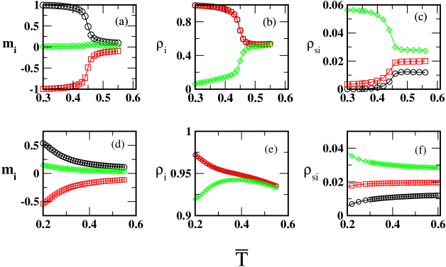
Figure 3: Sub-lattices distributions for solvent and solute properties for $2\%$ solute concentration and $\zeta=1/10$. From right to left, we have solvent particle orientation $m_{i}$ , solvent particle density $\rho_{i}$ and solute density $\rho_{si}$ versus reduced temperature $\overline{T}$ . Top graphs are for lower reduced chemical potential $\bar{\mu}=-1.6$, bottom graphs are for higher reduced chemical potential $\bar{\mu}=-0.4$. Colors identify sub-lattices.

Figure 4 displays the reduced chemical potential versus reduced temperature phase diagrams for $10\%$ concentration of the solute, for both values of hydrogen bond strength $\zeta=1/4$ (left) and $\zeta=1/10$ (right). In this case substantial change in the phase diagrams can be seen. The low temperature SL to NSL phase transition seen as one increases chemical potential for pure solvent is destroyed by the presence of solute. Instead, the transition may be reached only from temperature variations, and the SL phase extends to very high chemical potentials. The TMD line moves nearer to the critical SL-NSL line and crosses into the SL phase.

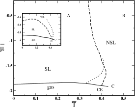
Figure 4: Solvent reduced chemical potential $\bar{\mu}$ versus reduced temperature $\bar{T}$ phase diagram for model solution at solute concentration $10\%$ for $\zeta=1/4$ and $\zeta=1/10$. Solid, dashed and dotted lines correspond to first-order, second-order phase transitions and the TMD, respectively. The symbols $CE$, $C$ and $t$ denote critical-ending, critical and tricritical points, respectively. The insets displays the corresponding phase diagrams for pure solvents for comparison.

In Fig. 5 we investigate the solvent orientation and density, as well as, the density of solute in each sublattice in different regions of the phase diagram at $10\%$ solute concentration for bond strength $\zeta=1/10$. For both low, $\bar{\mu}=-1.3$, and high, $\bar{\mu}=4.0$, reduced chemical potential, solute orders together with solvent at low temperatures. As can be seen from the color identification of lattices, solute goes into the empty lattice while solvent particles orient properly on two sub-lattice in order to connect through bonds.

For both reduced chemical potentials an abrupt variation of the solvent density, of the solute density and of the solvent orientation occur simultaneously, near $\bar{T}=0.45$ for $\bar{\mu}=-1.3$ and near $\bar{T}=0.3$ for $\bar{\mu}=4.0$ at the SL-NSL transition line.

However, despite of the qualitative similar behavior there are quantitative important differences between the two regions of chemical potential. For the lower chemical potential, $\bar{\mu}=-1.3$, solvent behavior is similar to that of pure solvent. The orientationally ordered solvent particles occupy mainly two of the sub-lattice, while the third sublattice remains nearly free of solvent. At $\bar{T}=0.3$ nearly $60\%$ of that sub-lattice stands vacant, while solute particles occupy $30\%$ of the sites, leaving the other two sub-lattice free of solute.

At high chemical potential, $\bar{\mu}=4.0$, while solute maintains the $30\%$ occupancy of one of the sub-lattice at low temperature, the solvent particles fill up the rest of the sublattice sites, reaching $70\%$ occupancy of that sublattice.

The new behavior induced by the presence of solute is better understood by comparing Fig. 3(e) and Fig. 5(e). Differently from the $2\%$ solute concentration, for the $10\%$ concentration case the filling up of the lattice yields only partial rupture of hydrogen-bonding. Maintenance of the hydrogen bond network at such high density seems to be a result of the structuring effect of solute.

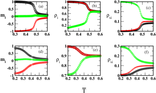
Figure 5: Solution structure in the new phase. Sub-Lattice solvent particle orientation $m_{i}$, solvent density $\rho_{i}$, and solute density $\rho_{si}$ vs. temperature for different chemical potentials for $10\%$ of solute concentration and $\zeta=1/10$. The top and bottom graphs correspond to solvent chemical potentials $\mu=-1.30$ and $\mu=4.0$.

Inspection of typical configurations in different regions of the phase diagrams are quite useful at this point. Fig. 7 and Fig. 6 display snapshots of the model system at different points (indicated by letters in Fig. 4) in the reduced chemical potential versus reduced temperature phase diagrams with solute concentration $10\%$.

For $\zeta=1/4$ (Fig. 6), at $\bar{\mu}=-0.50$ and $\bar{T}=0.25$ (inside SL phase, point A in Fig. 4 ), lattice is filled up, but patches of structured liquid can be seen with solute localizing only in sites which contribute to organize the hydrogen bond network. As the SL-NSL line is crossed and for $\bar{T}=0.50$ (point D in Fig. 4), a few isolated solute particles are surrounded by water particle structure, while most solute particles are clustered in vacant regions.

For $\zeta=1/10$ (Fig. 7), at $\bar{\mu}=-1.40$ and $\bar{T}=0.30<\bar{T}_{TMD}$ (point C in Fig. 4), a fully bonded network of solvent particles is accompanied by solute particles located in the empty sublattice. This gives rise to apparently linear aggregates intercalated by solvent. At a temperature higher than the TMD, $\bar{T}=0.50$ (point D in Fig. 4), some bonding of the solvent particles in hexagons are still seen, with intercalated solute.However, the system is much less dense, and solute particles also localize in large vacant regions.

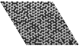
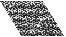
Figure 6: Snapshots of model system for concentration of $10\%$ and $\zeta=1/4$ at high chemical potential, $\bar{\mu}=-0.5$, in A ($\bar{T}=0.25$, left) and B ($\bar{T}=0.5$, right) points in Fig. 4. Black and Grey circles are two orientations of solvent particles, black dots represent solute particles.

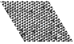
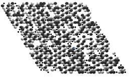
Figure 7: Snapshots of model system for concentration of $10\%$ and $\zeta=1/10$ at low chemical potential, $\bar{\mu}=-1.4$, in C ($\bar{T}=0.3$, left) and D ($\bar{T}=0.5$, right) points in Fig. 4. Black and gray circles are two orientations of solvent particles, black dots represent solute particles.

V Model solubility

The Ostwald solubility $\Sigma$ is defined as the ratio between solute densities $\rho_{X}$ in the two coexisting phases:

$$\Sigma=\frac{\rho_{X}^{I}}{\rho_{X}^{II}}.$$ (2)

The two coexisting phases, $I$ and $II$, might either be a gas phase $II$ that coexists with a homogeneous liquid phase $I$ Gu93 or two liquid phases $I$ and $II$, of different relative densities, the first poor in solute $X$, the other reach in $X$ Ba91 .

In the case of liquid-liquid phase separation, the form of the temperature-density coexistence curve, at fixed pressure, is indicative of solubility behavior. If the density gap decreases as temperature is increased, solubility increases with temperature. However, for reentrant coexistence curves, for which the density gap increases as temperature is increased, solubility decreases as temperature is raised.

On the other hand, minimal statistical models show that for dense lattice gas solutions with isotropic van der Waals-like interactions solubility behaves univocally with temperature. Coexistence densities between an ideal gas mixture and a lattice dense solution, for substances Y and X, are obtained from the equality of the corresponding chemical potentials. Consider interaction constants $w_{YY}$, $w_{XX}$ and $w_{YX}$ between pairs YY, XX and YX. For solute X in the gas phase given by the dimensionless solute X density $\rho_{X}^{gas}$, we might write

$$\mu_{X}^{gas}=k_{B}T\ln\rho_{X}^{gas},$$ (3)

whereas for solute X in the dense lattice solution, we have

$$\mu_{X}^{solution}=\frac{w_{XX}}{2}-\frac{w}{2}(1-x_{X})^{2}+k_{B}T\ln x_{X}^{solution},$$ (4)

where $w=w_{YY}+w_{XX}-2w_{YX}$ and $x_{X}$ is the solution concentration given in mole fraction. Equating Eq. (3) to Eq. (4) yields

$$\frac{x_{X}^{solution}}{\rho_{X}^{gas}}=e^{-\frac{\beta w_{XX}}{2}}e^{\frac{\beta w}{2}(1-x_{X}^{solution})^{2}}\;.$$ (5)

A slightly different definition of solubility, proportional to the inverse of Henry’s constant, is given by

$$\Sigma^{\prime}=\frac{x_{X}^{solution}}{\rho_{X}^{gas}/\rho_{X}^{0}},$$ (6)

where $\rho_{X}^{0}$ is gas density for pure liquid X. Comparing Eq. (5) with Eq. (6) gives

$$\Sigma^{\prime}=e^{\frac{\beta w}{2}(1-x_{X}^{solution})^{2}}.$$ (7)

Thus for poorly miscible solutions, with $w<0$, which phase separate at low temperatures, solubility increases with temperature, since $d\Sigma^{\prime}/dT\propto-w$. On the other hand, if the two liquids are miscible, when $w>0$, solubility decreases as temperature is raised. In either case, solubility displays monotonic behavior with temperature.

The solubility behavior of the dense lattice model is the result of a competition between entropy of mixture and an isotropic interaction potential. relies on positional entropy The model misses the role of density, an essential feature of water.

How does the introduction of asymmetry in the interaction potential, accompanied by orientational entropy, change this picture? In order to answer to this question we have measured the solubility of our model inert solute as a function of temperature for different fixed chemical potential of solvent, by assuming coexistence of a gas (phase $Y$) and a homogeneous solution phase ($X$). The gas phase was assumed ideal, thus

$$\mu_{X}^{gas}=-k_{B}T\ln\rho_{X}^{gas}.$$ (8)

For the solution phase, the chemical potential of solute was calculated from simulation data through Widom’s insertion method Wi63 . In our semi-grand canonical ensemble the semi-grand potential $\psi=\psi(T,V,N_{X},\mu)$ depends on $T$, $V$, $N_{X}$ and on the solvent chemical potential $\mu$. In the thermodynamic limit, the solute chemical potential $\mu_{X}^{solution}=-(\frac{\partial\psi}{\partial N_{X}})$ can be approximated by the difference $\psi(T,V,N_{X}+1,\mu)-\psi(T,V,N_{X},\mu)$ and we have

$$\mu_{X}^{solution}=-k_{B}T\ln\frac{\Xi(T,V,\mu,N_{X+1})}{\Xi(T,V,\mu,N_{X})},$$ (9)

which relates average values in two different ensembles of $N_{X}$ and $N_{X+1}$ particles. However, the numerator can be interpreted in terms of an average in the ensemble of $N_{X}$ solute particles. Thus we have

$$\mu_{X}^{solution}=-k_{B}T\ln\left(\frac{1}{\langle\rho_{X}^{solution}\rangle}\right)\langle e^{-\beta\Delta u}\rangle_{T,V,N_{X},\mu},$$ (10)

where $\Delta u$ is the additional energy due to insertion of solute molecule to a system of solute concentration $\rho_{X}^{solution}=N_{X}/V$. Finally, by equating $\mu_{X}^{solution}$ and $\mu_{X}^{gas}$, we obtain for the solubility

$$\Sigma=\frac{\rho_{X}^{solution}}{\rho_{X}^{gas}}=\langle e^{-\beta\Delta u}\rangle_{T,V,N_{X},\mu}.$$ (11)

In the Fig. 8 we display our data for solubility $\Sigma$ versus temperature for bond strength $\zeta=1/10$. As can be seen, a minimum is present for different chemical potential of solvent.

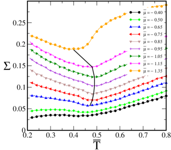
Figure 8: Ostwald coefficient $\Sigma$ versus $\overline{T}$ for different $\overline{\mu}$ for $\zeta=1/10$ and $10\%$. The black line corresponds the temperature for which the density presents a maximum.

The temperature of minimum solubility (TmS) coincides entirely with the temperature of maximum density (TMD), in the $\bar{\mu}$ vs. $\bar{T}$ plane. This is to be expected for inert solutes. Inspection of Eq. (11) for inert solutes yields $\exp\{-\beta\Delta u\}=1$ for insertion into empty sites and $0$, otherwise. Thus solubility can be directly related to the overall liquid density $(N_{X}+N^{solvent})/V$. Thus

$$\Sigma=\langle e^{-\beta\Delta u}\rangle_{T,V,N_{X},\mu}=1-\rho^{solvent}-\rho_{X}^{solute},$$ (12)

and for fixed solute density

$$\frac{d\Sigma}{dT}=-\frac{d\rho^{solvent}}{dT},$$ (13)

and therefore the TMD is accompanied by the TmS. Is the coincidence between TmS and TMD restricted to inert solutes?

It is tempting to extend our analysis of Eq. (11) to interacting solutes. A first simplest approach to the question would be to investigate the energetic effect on solubility through the following approximation

$$\Sigma=\langle e^{-\beta\Delta u}\rangle_{T,V,N_{X},\mu}\approx(1-\rho^{solvent}-\rho_{X}^{solute})e^{-\beta<\Delta u>},$$ (14)

thus

$$\frac{d\Sigma}{dT}\approx\left[-\frac{d\rho^{solvent}}{dT}+(1-\rho^{solvent}-\rho_{X}^{solute})\left(\frac{<\Delta u>}{k_{B}T^{2}}-\beta\frac{d<\Delta u>}{dT}\right)\right]e^{-\beta<\Delta u>}.$$ (15)

Since $<\Delta u>$ is necessarily negative and $\frac{d<\Delta u>}{dT}$ is necessarily positive, this result implies that the minimum in solubility should occur at a temperature higher than TMD. This is in accordance with data on solubility of gases.

VI Conclusions

In this paper we have considered the investigation of the thermodynamic phases and of solubility of the Bell-Lavis (BL) water model in the presence of small inert solute. The Bell-Lavis two-dimensional orientational model presents a density anomaly and two liquid phases of different structure.

We have considered two fixed concentrations of solute, respectively $2\%$ and $10\%$. In both cases, but more evidently for $10\%$ solute, the presence of solute ’strengthens’ the hydrogen bonds. Inspection and comparison of phase diagrams show that the structured phase is stabilized to higher temperatures, at fixed chemical potential, and to much higher chemical potentials. For the higher concentration of solute, the transition between the structured and the unstructured phases as chemical potential is varied disappears. Examination of solvent structure shows that the presence of solute nucleates patches of hydrogen-bonded solvent particles. Solute intercalates with properly oriented solvent. Both features, increment of water structure and solvent-separated solute states, have been reported from experiments and atomistic models La93 .

Solubility of our small inert solutes presents a minimum (TmS), which coincides with the maximum solvent density (TMD), as expected Pr77 . For interacting solute, a simple argument leads us to expect TmS to occur at higher temperatures for the BL solvent model.

Investigation of the latter point, as well as the effect of solute size are the subject of ongoing work.

References

- (1) T. L. Hill, Statistical Thermodynamics, Addison-Wesley Pub., New York, NY, 1960.
- (2) H. R. Batino, R. anda Clever, Chem. Rev. 66, 395 (1966).
- (3) J. D. Bernal and R. H. Fowler, J Chem. Phys. 1, 515 (1913).
- (4) T. Head-Gordon and G. Hura, Chem. Rev. 102, 2651 (2002).
- (5) J. B. Perrin, C. L. anda Nielson, Annu. Rev. Phys. Chem. 48, 511 (1997).
- (6) N. A. M. Besseling and J. Lyklema, J. Phys. Chem. 98, 11610 (1994).
- (7) G. M. Bell and D. A. Lavis, J. Phys. A 3, 568 (1970).
- (8) S. Sastry, P. G. Debenedetti, and F. Sciortino, Phys. Rev. E 53, 6144 (1996).
- (9) C. J. Roberts and P. G. Debenedetti, J. Chem. Phys. 105, 658 (1996).
- (10) G. Franzese and H. E. Stanley, J. Phys.: Cond. Matter 14, 2201 (2002).
- (11) M. Pretti and C. Buzano, J. Chem. Phys 121, 11856 (2004).
- (12) E. Lomba, N. G. Almarza, C. Martin, and C. McBride, J. Chem. Phys. 126, 244510 (2007).
- (13) N. G. Almarza, J. A. Capitan, J. A. Cuesta, and E. Lomba, J. Chem. Phys 131, 124506 (2009).
- (14) P. C. Hemmer and G. Stell, Phys. Rev. Lett. 24, 1284 (1970).
- (15) E. A. Jagla, Phys. Rev. E 58, 1478 (1998).
- (16) M. C. Wilding and P. F. McMillan, J. Non-Cryst. Solids 293, 357 (2001).
- (17) P. Camp, Phys. Rev. E 68, 061506 (2003).
- (18) V. N. Ryzhov and S. M. Stishov, Phys. Rev. E 67, 010201 (2003).
- (19) D. Y. Fomin et al., J. Chem. Phys 129, 064512 (2008).
- (20) G. Franzese, G. Malescio, A. Skibinsky, S. V. Buldyrev, and H. E. Stanley, Nature (London) 409, 692 (2001).
- (21) A. B. de Oliveira, P. A. Netz, T. Colla, and M. C. Barbosa, J. Chem. Phys. 124, 084505 (2006).
- (22) N. Barraz Jr., E. Salcedo, and M. Barbosa, J. Chem. Phys. 131, 094504 (2009).
- (23) A. B. de Oliveira et al., J. Chem. Phys. 132, 164505 (2010).
- (24) V. B. Henriques and M. C. Barbosa, Phys. Rev. E 71, 031504 (2005).
- (25) C. E. Fiore, M. M. Szortyka, M. C. Barbosa, and V. B. Henriques, J. Chem. Phys. 131, 164506 (2009).
- (26) M. M. Szortyka, M. Girardi, V. B. Henriques, and M. C. Barbosa, J. Chem. Phys. 132, 134904 (2010).
- (27) M. M. Szortyka, C. E. Fiore, V. B. Henriques, and M. C. Barbosa, J. Chem. Phys. 133, 104904 (2010).
- (28) L. R. Pratt and D. Chandler, J. Chem. Phys. 67, 3683 (1977).
- (29) B. J. Berne, Proc. Natl. Acad. Sci. 93, 8800 (1996).
- (30) G. G. Hummer, S. Garde, A. E. García, A. Pohorille, and L. R. Pratt, Proc. Natl. Acad. Sci. 93, 8951 (1996).
- (31) B. Guilot and Y. Guissani, J. Chem. Phys. 99, 8075 (1993).
- (32) M. A. A. Barbosa and V. B. Henriques, Phys. Rev. E 77, 051204 (2008).
- (33) F. S. Bates, Science 251, 898 (1991).
- (34) B. Widom, J. Phys. Chem. 39, 11 (1963).
- (35) C. Buzano, E. B. De Stefanis, and M. Pretti, Phys. Rev. E 71, 051502 (2005).
- (36) B. M. Laadanyi and M. S. Skaf, Annu. Rev. Phys. Chem. 44, 3335 (1993).