Insights into the Nucleon Spin from Lattice QCD

Abstract

Flavour singlet contributions to the nucleon spin are elusive due to the fact that they cannot be determined directly in experiment but require extrapolations to the small x region. Direct calculations of these contributions are possible using Lattice QCD, however, they pose a significant computational challenge due to the presence of disconnected quark line diagrams. We report on recent progress in determining these sea quark contributions on the lattice.

1 Introduction and Results

The distribution of the spin of the proton among its constituents has long been a topic of interest. The total spin can be decomposed into the contribution from the quark spins, $\Delta\Sigma$, the quark orbital angular momenta, $L_{\psi}$, and the gluon total angular momentum $J_{g}$ [1],

$$\frac{1}{2} = \frac{1}{2}\Delta\Sigma+L_{\psi}+J_{g},$$ (1)

where $\Delta\Sigma=\Delta u+\Delta d+\Delta s$ (heavier quarks are normally neglected). In this work, $\Delta q$ ($q=u,d,s$) denotes the combined spin contribution of the quark and the antiquark. Using Lattice QCD, one can determine the $\Delta q$ from first principles through the axial-vector matrix element,

$$\frac{1}{m_{N}}\langle N,s|\bar{q}\gamma_{\mu}\gamma_{5}\frac{1}{2}q|N,s\rangle = \frac{\Delta q}{2}\hskip 2.84544pts_{\mu},$$ (2)

where $m_{N}$ is the mass of the nucleon with spin $s_{\mu}$ ($s_{\mu}^{2}=-1)$. Thus, one can construct the axial charges, $a_{3}=\Delta u-\Delta d=g_{A}$, $a_{8}=\Delta u+\Delta d-2\Delta s$ and $a_{0}(Q^{2})=\Delta u+\Delta d+\Delta s=\Delta\Sigma(Q^{2})$. $\Delta\Sigma$ acquires a scale dependence, $Q^{2}$, due to the axial anomaly. The axial-vector matrix element is related to the first moment of the quark helicity distributions. The second moment, $\langle x\rangle_{\Delta}$, and the second moment of the transverse helicity distribution, $\langle x\rangle_{\delta}$, can also be calculated on the lattice, higher moments are more challenging. Furthermore, the total angular momentum of quark $q$, $J_{q}=\frac{1}{2}\Delta q+L_{q}$ ($\sum_{q}J_{q}=\frac{1}{2}\Delta\Sigma+L_{\psi}$) can be obtained from the generalised form factors, $A^{q}_{20}(Q^{2})$ and $B^{q}_{20}(Q^{2})$, which parameterise the matrix element of the energy-momentum tensor for momentum transfer, $Q$. For a review of recent Lattice results of $J_{q}$, $\langle x\rangle_{\Delta}$ and $\langle x\rangle_{\delta}$ see [2, 3] and references therein.

In these proceedings we focus on $\Delta q$ and $\Delta s$ in particular. Lattice results for $\Delta s$ have an important role to play in constraining fits of polarised parton distribution functions (PDF). The spin structure function of the proton and neutron, $g^{n,p}_{1}(x,Q^{2})$, is measured in deep inelastic experiments. The first moment is related to the axial charges via the operator product expansion. To leading twist:

$$\Gamma^{p,n}_{1}(Q^{2})=\int_{0}^{1}\mathrm{d}x\,g_{1}^{p,n}(x,Q^{2}) = \frac{1}{36}\left[(a_{8}\pm 3a_{3})C_{NS}+4a_{0}C_{S}\right]$$ (3)

where $C_{S}$ and $C_{NS}$ are the singlet and non-singlet Wilson coefficients, respectively. Model assumptions are made in order to extrapolate $g^{n,p}_{1}(x,Q^{2})$ from the minimum $x=0.02$ accessible in experiment down to $x=0$. $a_{3}$ is known from neutron $\beta$-decay, while, assuming $SU(3)$ flavour symmetry, $a_{8}$ can be obtained from hyperon $\beta$-decays. Thus, in combination with $\Gamma^{p,n}_{1}(Q^{2})$, $a_{0}$ and the $\Delta q$ can be deduced. For example, HERMES find $\Delta s(5\mathrm{GeV}^{2})=\frac{1}{3}(a_{0}-a_{8})=-0.085(13)(8)(9)$ [4]. However, if the range of $x$ in the integral in Eq. 3 is restricted to the experimental range, $x>0.02$, $\Delta s$ is consistent with zero, indicating the large negative value arises from model assumptions in the low $x$ region.

Semi-inclusive deep inelastic scattering (SIDIS) experiments offer a direct measurement of the $\Delta q$ using pion and kaon beams. Results from COMPASS show the strangeness contribution is consistent with zero down to $x=0.004$ [5]. A naive extrapolation to $x=0$ gives $\Delta s=-0.02(2)(2)$, while using the parameterisation of De Florian et al. (DSSV) [6] gives $\Delta s=-0.10(2)(2)$. Present measurements via SIDIS are limited by the knowledge of the quark fragmentation functions, to which $\Delta s$ is particularly sensitive. Another possibility of directly determining $\Delta s$ combines $\nu p$, $\bar{\nu}p$ and parity-violating $ep$ elastic scattering data [7]. Here, the MicroBooNE experiment will enable errors to be significantly reduced.

Considering the lattice approach, simulations are performed at finite volume ($V$) and lattice spacing ($a$) and typically with $u$ and $d$ quarks with unphysically heavy masses ($m_{q}$). Physical results are recovered in the continuum ($a\to 0$) and infinite volume ($V\to\infty$) limits at physical quark masses. The $u$, $d$ and $s$ quark masses used in simulations are normally expressed in terms of the pseudoscalar meson masses they correspond to ($M_{PS}^{2}\propto m_{q}$). Developments in algorithmic techniques and computing power mean typical simulations now involve lattices with $a\sim{0.05-0.1}$ fm, $V\sim 2.5-6$ fm and $M_{PS}(u/d)\sim 200$ MeV.

For any lattice prediction, the size of the main systematic errors, discretisation effects, finite volume and so on, must be investigated thoroughly. However, the systematic uncertainties should always be compared to the inherent statistical error, where for some quantities the latter dominates. $\Delta s$ is one such example. Evaluating $\langle N|\bar{s}\gamma_{\mu}\gamma_{5}s|N\rangle$ involves calculating a disconnected quark line diagram (for the strange quark). These types of diagrams are computationally expensive to calculate as they involve the quark propagator from all space-time lattice points to all points. In the past these diagrams were often not calculated and differences of quantities were quoted, for which the disconnected contribution cancelled assuming isospin symmetry, for example, $g_{A}=\Delta u-\Delta d$, $J_{u-d}$ and $\langle x\rangle_{\Delta u-\Delta d}$. However, methods have been developed which enable the disconnected contributions to be calculated [8], in particular, also $\Delta s$. Note that for $\Delta u$ and $\Delta d$ a “connected” quark line diagram must also be evaluated in addition to the disconnected one.

In the following we present results for the quark spin contributions to the proton generated on configurations with two degenerate flavours of sea quarks, with $a\sim 0.072$ fm and $u/d$ quark masses given by $M_{PS}=285$ MeV. The quark action employed has leading order discretisation effects of $O(a^{2})$, which are not expected to be significant for this value of the lattice spacing. Two lattice volumes, with spatial dimensions of $2.3$ fm and $2.9$ fm, were used and no significant finite volume effects were found. Although the $u$ and $d$ quark masses are unphysically heavy, we varied the quark masses in the range corresponding to $M_{PS}=285-720$ MeV and found no significant change in the results. This suggests our results may also apply to physical quark masses. Further details can be found in [9].

$q$	$\Delta q^{\mathrm{lat}}_{\rm con}$	$\Delta q^{\mathrm{lat}}_{\rm dis}$	$\Delta q^{\mathrm{\overline{MS}}}(Q)$	DSSV $x_{min}$	DSSV $0$
$u$	1.071(15)	-0.049(17)	0.787(18)(2)	0.793	0.814
$d$	-0.369( 9)	-0.049(17)	-0.319(15)(1)	-0.416	-0.458
$s$	0	-0.027(12)	-0.020(10)(1)	-0.012	-0.114
$a_{3}$	1.439(17)	0	1.105(13)(2)	1.21	1.272
$a_{8}$	0.702(18)	-0.044(19)	0.507(20)(1)	0.401	0.583
$\Sigma$	0.702(18)	-0.124(44)	0.448(37)(2)	0.366	0.242

Table 1: The bare (lattice) connected, $\Delta q^{\mathrm{lat}}_{\rm con}$, and disconnected, $\Delta q^{\mathrm{lat}}_{\rm dis}$, quark spin contributions of the proton. Renormalisation to the $\mathrm{\overline{MS}}$ scheme is performed for $Q\sim\sqrt{7.4}$ GeV, to obtain $\Delta q^{\mathrm{\overline{MS}}}(Q)$. The first error is statistical, the second is from the renormalisation. A comparison is made with the results of DSSV global fits to DIS and SIDIS data [10] (see this reference for the uncertainties on the values) for the cases where $x$ is restricted to $\left[x_{min}=0.001\to 1\right]$ and where $x=\left[0\to 1\right]$.

Table 1 displays the results for $\Delta s$ and the axial charges and compares them to results from a DSSV global analysis [10]. We obtain a small, negative value for $\Delta s$, consistent with the result obtained from a truncated DSSV fit to experimental data. Notably, $a_{3}$ is significantly lower than the experimental value of $a_{3}=g_{A}=1.2695(29)$. This is a general feature of lattice calculations of $g_{A}$. A summary plot of recent simulations taken from [3] is shown in Fig. 1. Over the range of $u/d$ quark masses available the results obtained using different lattice quark actions, volumes and lattice spacings, are fairly constant and lie approximately $10\%$ below the experimental result. Simulations at smaller $u/d$ quark masses are needed. Problems with excited state contaminations have also been suggested as a possible source of the discrepancy, see, for example, Ref. [11]. On the lattice an operator with the quantum numbers of the proton, creates all states of $J^{P}=\frac{1}{2}^{+}$ and one needs to ensure that the matrix element for the ground state has been extracted. Nonetheless, the uncertainty in the lattice determination of $g_{A}$ seems to be multiplicative, as shown on the right in Fig. 1: the ratio of $g_{A}/f_{\pi}$ tends to the experimental value.

Considering the underestimate of $g_{A}$, we add a $20\%$ uncertainty to our results and obtain a final value of

$$\Delta s=-0.020(10)(4).$$

The first error is statistical, the second is due to the systematic uncertainty, which dominates. Other groups using similar methods, albeit at heavier quark masses and without renormalisation, obtain consistent results, see [12] and [13]. This is in contradiction to earlier exploratory work by, for example, the Kentucky group [14]. Note that this group have recently also calculated flavour singlet contributions to $J_{q}$ [15].

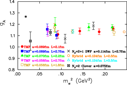
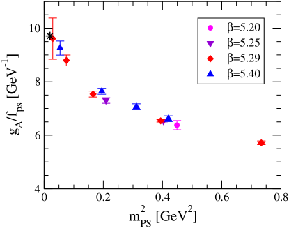
Figure 1: (left) A summary plot of $a_{3}=g_{A}$ for different lattice simulations as a function of the $u/d$ quark mass, expressed in terms of $M_{PS}^{2}=m_{\pi}^{2}$ [3]. (right) The ratio of $g_{A}/f_{\pi}$ as a function of $M_{PS}^{2}$ for different lattice spacings [16]. $\beta=5.2-5.4$ corresponds to $a\sim 0.083-0.060$ fm.

2 Acknowledgements

This work is supported by the EU ITN STRONGnet and the DFG SFB/TRR 55. S.C. acknowledges support from the Claussen-Simon-Foundation (Stifterverband für die Deutsche Wissenschaft).

References

- [1] X.-D. Ji. Phys.Rev.Lett. 78 (1997) 610–613, arXiv:hep-ph/9603249 [hep-ph].
- [2] P. Hagler. Phys.Rept. 490 (2010) 49–175, arXiv:0912.5483 [hep-lat].
- [3] C. Alexandrou. Prog. Part. Nucl. Phys. 67 (2012) 101–116, arXiv:1111.5960 [hep-lat].
- [4] A. Airapetian et al. Phys. Rev. D75 (2007) 012007, arXiv:hep-ex/0609039 [hep-ex].
- [5] M. Alekseev et al. Phys. Lett. B693 (2010) 227–235, arXiv:1007.4061 [hep-ex].
- [6] D. de Florian, R. Sassot, M. Stratmann, and W. Vogelsang. Phys.Rev.Lett. 101 (2008) 072001, arXiv:0804.0422 [hep-ph].
- [7] S. F. Pate. Phys.Rev.Lett. 92 (2004) 082002, arXiv:hep-ex/0310052 [hep-ex].
- [8] G. S. Bali, S. Collins, and A. Schafer. Comput.Phys.Commun. 181 (2010) 1570–1583, arXiv:0910.3970 [hep-lat].
- [9] G. S. Bali et al. arXiv:1112.3354 [hep-lat].
- [10] D. de Florian, R. Sassot, M. Stratmann, and W. Vogelsang. Phys. Rev. D80 (2009) 034030, arXiv:0904.3821 [hep-ph].
- [11] S. Capitani, M. Della Morte, G. von Hippel, B. Jager, A. Juttner, et al. arXiv:1205.0180 [hep-lat].
- [12] R. Babich, R. C. Brower, M. A. Clark, G. T. Fleming, J. C. Osborn, et al. Phys. Rev. D85 (2012) 054510, arXiv:1012.0562 [hep-lat].
- [13] M. Engelhardt. PoS LATTICE2010 (2010) 137, arXiv:1011.6058 [hep-lat].
- [14] S. Dong, J.-F. Lagae, and K. Liu. Phys.Rev.Lett. 75 (1995) 2096–2099, arXiv:hep-ph/9502334 [hep-ph].
- [15] K. Liu, M. Deka, T. Doi, Y. Yang, B. Chakraborty, et al. arXiv:1203.6388 [hep-ph].
- [16] D. Pleiter et al. PoS LATTICE2010 (2010) 153, arXiv:1101.2326 [hep-lat].