Keeping greed good: sparse regression under design uncertainty with application to biomass characterization

Abstract

In this paper, we consider the classic measurement error regression scenario in which our independent, or design, variables are observed with several sources of additive noise. We will show that our motivating example’s replicated measurements on both the design and dependent variables may be leveraged to enhance a sparse regression algorithm. Specifically, we estimate the variance and use it to scale our design variables. We demonstrate the efficacy of scaling from several points of view and validate it empirically with a biomass characterization data set using two of the most widely used sparse algorithms: least angle regression (LARS) and the Dantzig selector (DS).

1 Introduction

This paper is motivated by the practical problem of how to meaningfully perform sparse regression when the predictor variables are observed with measurement error or some source of uncertainty. We will refer to this error or noise as design uncertainty to emphasize that perturbations in the design matrix may arise from a number of random sources unrelated to experimental or measurement error per se. Recent work in this area has just begun to address the issue of sparse regression under design uncertainty from a theoretical point of view. We are primarily interested in describing an approach that, while theoretically justifiable, is essentially pragmatic and broadly applicable. In short, we argue that greed - a basic feature of many sparsity promoting algorithms - is indeed good (Tropp, 2004), so long as the design data is scaled by the uncertainty variances. We demonstrate the efficacy of scaling from several points of view and validate it empirically with a biomass characterization data set using two of the most widely used sparse algorithms: least angle regression (LARS) and the Dantzig selector (DS).

Our work was motivated by an example from a biomass characterization experiment related to work at the National Renewable Energy Laboratory. The example is described in detail in Section 4 and contains repeated measurements of mass spectral (design, or predictor) and sugar mass fraction (response) values within each switchgrass sample. The domain scientists’ goal was to find a small subset of masses in the spectrum that could be used to predict sugar mass fraction. We will show that the replication of each measurement allows for simple estimates of the error variances which, in turn, may be used to guide the model selection procedure. Thus, we are interested in sparse regression under design uncertainty. We would also like for a scientist examining the model to have some hope of interpreting its meaning, either for immediate understanding or to indicate new research directions.

Sparse regression by $l_{1}$ minimization is a thriving and relatively young field of research. In the statistical inference literature, early stepwise-type algorithms paved the way for the now-familiar lasso (Tibshirani, 1996), least angle regression (LARS) (Efron et al., 2004), and many variants tailored to specific problems (for example, Yuan and Lin (2006); Zou and Hastie (2005); Tibshirani and Taylor (2011); Hastie et al. (2007); Percival et al. (2011)). A parallel evolution in the signal processing literature led to the development of widely used basis and matching pursuit algorithms (Chen et al., 1998, 2001; Tropp, 2004), the Dantzig selector (DS) (Candes and Tao, 2007), and many others (see, e.g., Elad (2010), Chapters 3 and 5, for a good overview). Despite their mostly independent development, the algorithms coming out of the statistical and signal processing worlds lead to remarkably similar results in many applications (e.g., Bickel et al. (2009)).

Linear regression under the assumption of design uncertainty has, in comparison, a long history, going by various names such as error in variables or functional modeling, and a variety of techniques have been developed to address it (e.g., Gillard (2010); Fuller (1987, 1995)). Until fairly recently, however, much of the analysis of sparse representations has not confronted this issue. As we will discuss, there is good reason for this, namely, that this problem obfuscates the goal of sparse regression.

Several recent works that have looked at sparse regression under various assumptions about the noise should be mentioned. Rosenbaum and Tsybakov (2010), develop a Dantzig-like estimator that they argue is more stable than the standard lasso or Dantzig. Sun and Zhang (2011) describe an algorithm to estimate the lasso solution and the noise level simultaneously. A similar idea, leading to the “adaptive lasso”, was developed by Huang et al. (2008) under homoscedastic assumptions. An algorithm that hybridizes total least squares (Golub and Loan, 1980), a computational error in variables model, and the lasso was also recently published by Zhu et al. (2011).

The work that comes nearest to our discussion is by Wagener and Dette (2011a, b). In these papers, the authors present some asymptotic results for bridge and lasso estimators under the assumption of heteroscedasticity. In particular, they develop a weighting scheme that leads to adaptive lasso estimates that are sign consistent (i.e., they satisfy the “oracle property”).

We consider this paper to be somewhat disjoint from the aforementioned for two reasons. First, we are primarily concerned with an approach that incorporates empirical knowledge of design uncertainty into the analysis. Second, we wish to argue from a more general, and necessarily more heuristic, point of view that does not require stringent conditions, such as those described by Wagener and Dette (2011a), Section 3, to hold. In other words, we want to allow for the possibility that the data that is given to us may be “messy.” For example, we do not expect the design matrix to satisfy the restricted isometry property or to have low mutual coherence which, under certain circumstances, would guarantee the efficacy of an appropriate sparse algorithm.

A central notion throughout this paper is that many of the standard sparse regression algorithms are greedy, that is, they search for a solution incrementally, using the best available update at any given point in the search. As such, we argue that estimates of uncertainty should modify the notion of greed. Some algorithms, such as orthogonal matching pursuit (OMP), basis pursuit (BP), and forward stagewise regression (FS), are explicitly greedy. Others, like those that solve the lasso and Dantzig selector problems, may also be viewed as greedy via their connection to homotopy methods (Asif and Romberg, 2009, 2010; Efron et al., 2004). These methods generally take an initial estimate of the solution and move along a continuous path to the final one, choosing the best available search direction at each step.

Initially, we take forward stagewise (FS) regression as our prototype for analysis, noting its close relationship to the lasso and LARS (Hastie et al., 2007), as well as OMP and BP (Elad, 2010). We show that for all solution paths of a fixed norm, the uncertainty of the residual and the solution norm have a dual-like relationship in which the homogeneity of one induces inhomogeneity of the other, and that one can move from one problem to the other via a scaling of the design variables. From the standpoint of sparse pursuit, we argue that, as a general principle, uniform growth of the uncertainty along the solution path is preferable to uniform growth of the solution norm. Similar arguments are shown to apply to the Dantzig selector (DS). We then compare LARS and DS cross-validated model selection on a repeated measures biomass characterization data set in which variances are estimated via an analysis of variance (ANOVA) model. In this application, scaling by the uncertainty variance leads to sparser and more accurate models. Prediction error is reduced even further if, after down-selection of the variables by LARS and DS, the solution is updated via an $l_{2}$ method such as ridge regression.

2 Regression under design uncertainty

In this section, we formulate the model of interest and outline the challenges posed by design uncertainty. More importantly, we derive a simple estimate of this quantity which will play a central role in the discussion. We also give a simple example that illustrates how a very sparse solution can sometimes be associated with more of the design uncertainty than a less sparse one, further motivating our approach.

2.1 Model

We consider response data of the form,

$$y_{i} = w_{i}+\epsilon_{i},$$ (2.1)

$$w_{i} \sim N(0,\sigma_{w}^{2}),$$

$$\epsilon_{i} \sim N(0,\sigma_{\epsilon}^{2}),$$

$$\mbox{Cov}(\boldsymbol{w},\boldsymbol{\epsilon}) = 0,$$

and design data,

$$x_{ij} = v_{ij}+\delta_{ij},$$ (2.2)

$$v_{ij} \sim N(0,\sigma_{v_{j}}^{2}),$$

$$\delta_{ij} \sim N(0,\sigma_{\delta_{j}}^{2}),$$

$$\mbox{Cov}(\boldsymbol{v}_{j},\boldsymbol{\delta}_{j}) = 0,\,\,\,\,\,\,\,\,\,\,\,\,\forall j$$

for $1\leq i\leq n$ and $1\leq j\leq p$. The assumptions on $\mathbf{w}$ and $\mathbf{v}_{j}$ imply that the data are mean centered, and we interpret $\boldsymbol{\epsilon}$ and $\boldsymbol{\delta}_{j}$ as independent uncertainties,

$$\mbox{Cov}(\boldsymbol{\epsilon},\boldsymbol{\delta}_{j}) = 0,\,\,\,\forall j,$$

$$\mbox{Cov}(\boldsymbol{\delta}_{j},\boldsymbol{\delta}_{k}) = 0,\,\,\,j\neq k,$$

arising from measurement error, natural within-sample variability, or other random sources.

We will often express the system in matrix form,

$$\mathbf{y} = \mathbf{w}+\boldsymbol{\epsilon},$$

$$X = V+\Delta,$$

where $\boldsymbol{\epsilon}=(\epsilon_{1},\epsilon_{2},\dots,\epsilon_{n})^{\prime}$ and $\Delta=[\delta_{ij}]_{n\times p}$, and take the columns of $X$ and $\mathbf{y}$ to be scaled to unit variance, leading to the constraints

$$\sigma_{w}^{2}+\sigma_{\epsilon}^{2} = 1,$$

$$\sigma_{v_{j}}^{2}+\sigma_{\delta_{j}}^{2} = 1,\,\,\,\,\,\forall j.$$

Furthermore, we have

$$\mbox{Cov}(X) = \mbox{Cov}(V)+\Sigma^{2},$$

where $\Sigma^{2}\equiv\mbox{Cov}(\Delta)=\mbox{diag}(\sigma_{\delta_{1}}^{2},\sigma_{\delta_{2}}^{2},\dots,\sigma_{\delta_{p}}^{2})$ by the independence of the errors. When using finite sample estimates $s_{\delta_{j}}^{2}$ of $\sigma_{\delta_{j}}^{2}$, we denote the corresponding matrix by $S^{2}$. In the absence of noise ($\sigma_{\epsilon}^{2}=0$ and $\sigma_{\delta_{j}}^{2}=0,\,\forall j$), we assume that the design and response admit a linear model,

$$\mathbf{w}=V\boldsymbol{\beta}.$$ (2.3)

We are particularly interested in the case where $\boldsymbol{\beta}$ is sparse: loosely speaking, many of its elements are zero.

In the application discussed in Section 4, repeated measurements are used to estimate the variances $\sigma_{\delta_{j}}^{2}$. For a more theoretical application, it may be the case that these parameters are known exactly. Either way, for the remainder of the discussion we assume that either the variances or their sample estimates are available.

2.2 The challenge of design uncertainty

One intrinsic challenge in working with noisy design data is that the estimated regression coefficients are attenuated from their true values. Suppose, instead of (2.3), we were to solve

$$\mathbf{y}=X\boldsymbol{\beta}$$ (2.4)

via ordinary least squares (OLS) to obtain $\hat{{\beta}}$. For $p=1$, it is straightforward to show that

$$\frac{\mathbb{E}\{\hat{\beta}\}}{\beta}=\frac{\sigma_{\nu}^{2}}{\sigma_{\nu}^{2}+\sigma_{\delta}^{2}}<1,$$ (2.5)

where $\mathbb{E}$ denotes expected value. This implies that the estimators are biased towards zero by an amount that depends on the signal-to-noise ratio, $\sigma_{\nu}^{2}/\sigma_{\delta}^{2}$. More generally, for any full rank $X\in\mathbb{R}^{n\times p}$ with $n\geq p$, $X$ may be diagonalized such that in the new system of coordinates an analogous result holds.

Design uncertainty also degrades the model fit even if the exact solution $\boldsymbol{\beta}$ is known. To see this, consider the residual error when design uncertainty is present:

$$\mathbb{E}\{||\mathbf{y}-X\boldsymbol{\beta}||_{2}^{2}\} = \mathbb{E}\{||(\mathbf{w}+\boldsymbol{\epsilon})-(V+\Delta)\boldsymbol{\beta}||_{2}^{2}\}$$

$$= \mathbb{E}\{||\boldsymbol{\epsilon}-\Delta\boldsymbol{\beta}||_{2}^{2}\}$$

$$= \mathbb{E}\{\boldsymbol{\epsilon}^{\prime}\boldsymbol{\epsilon}-2\boldsymbol{\epsilon}^{\prime}\Delta\boldsymbol{\beta}+\boldsymbol{\beta}^{\prime}\Delta^{\prime}\Delta\boldsymbol{\beta}\}$$

$$= \sigma_{\epsilon}^{2}+\boldsymbol{\beta}^{\prime}\mathbb{E}\{\Delta^{\prime}\Delta\}\boldsymbol{\beta}$$

$$= \sigma_{\epsilon}^{2}+\boldsymbol{\beta}^{\prime}\Sigma^{2}\boldsymbol{\beta}$$

$$= \sigma_{\epsilon}^{2}+||\Sigma\boldsymbol{\beta}||_{2}^{2},$$

where we have explicitly used (2.3) and the independence of the errors.

This brings us to a main point, that the contribution of the design uncertainty to the residual is of the form $||\Sigma\boldsymbol{\beta}||_{2}^{2}$, which is quadratic in $\Sigma$. While we may only have access to the attenuated estimate $\hat{\boldsymbol{\beta}}$ of $\boldsymbol{\beta}$, the structure of the residual error remains the same with respect to the error variances. We illustrate the effect this can have on sparse regression with a simple example.

Example.

Suppose $p=3$ and

$$\mathbf{w} = v_{1},$$

$$v_{1} = \frac{1}{\sqrt{2}}(v_{2}+v_{3}),$$

$$\sigma_{\epsilon}^{2} = 0,$$

$$\Sigma^{2} = \mbox{diag}(\frac{1}{2},\frac{1}{4},\frac{1}{4}).$$

The system admits the two solutions $\boldsymbol{\beta}^{(1)}=(1,0,0)^{\prime}$ and $\boldsymbol{\beta}^{(2)}=\frac{1}{\sqrt{2}}(0,1,1)^{\prime}$. The first solution is the sparsest but in light of (2.2) has greater expected error since $||\Sigma\boldsymbol{\beta}^{(1)}||_{2}=1/2$ while $||\Sigma\boldsymbol{\beta}^{(2)}||_{2}=\sqrt{2}/4$. Hence, recovery of the sparsest solution results in greater uncertainty in the fit than the less sparse one. The issue becomes even more prominent - and more difficult to track - in higher dimensions with non-trivial covariance of the design matrix.

Apparently, greed is not always good under design uncertainty.

3 Scaling penalizes design uncertainty in the solution path

In this section, we briefly describe a prototypical greedy algorithm for sparse regression, forward stagewise regression (FS). We do so because it is helpful to have a particular algorithm in mind for the discussion, and this one is particularly easy to understand. In addition, it solves the widely-used lasso optimization problem and thus is closely related to a variety of other important algorithms (Efron et al., 2004; Hastie et al., 2007). Next, we state the main result and provide simple algebraic and geometric interpretations of it. Finally, we note implications of the result for the Dantzig selector problem.

3.1 A prototypical pursuit algorithm: forward stagewise (FS) regression

The FS algorithm may be summarized as follows:

1. Fix small $\gamma>0$ and initialize: $\hat{\boldsymbol{\beta}}=\mathbf{0}$, $\mathbf{r}=\mathbf{y}$.

2. Identify the design variable $\mathbf{x}_{j}$ most correlated with $\mathbf{r}$.

3. Incremental update : $\hat{\beta}_{j}\leftarrow\hat{\beta}_{j}+\eta_{j}$, where $\eta_{j}=\gamma\cdot\mbox{sign}(\mbox{Corr}(\mathbf{x}_{j},\mathbf{r})).$

4. Subtract the projection of $\mathbf{r}$ onto $\mathbf{x}_{j}$: $\mathbf{r}\leftarrow\mathbf{r}-\eta_{j}\mathbf{x}_{j}$.

5. If the residual norm is small enough, stop. Otherwise, return to step 2.

Qualitatively, the algorithm finds the best search direction - the coordinate with highest residual correlation - and takes a small step in that direction. It does so iteratively, updating the solution and residual at each step, until the minimal residual error is reached.

As an optimization procedure, FS regression (like the lasso and LARS) implicitly solves

$$\arg\min_{\boldsymbol{\beta}\in\mathbb{R}^{p}}\frac{1}{2}||\mathbf{y}-X\boldsymbol{\beta}||_{2}^{2}\,\,\,\,\,\mbox{subject to}\,\,\,\,\,||\boldsymbol{\beta}||_{1}<\lambda,$$ (3.1)

which is often expressed in Lagrangian form,

$$\arg\min_{\boldsymbol{\beta}\in\mathbb{R}^{p}}\frac{1}{2}||\mathbf{y}-X\boldsymbol{\beta}||_{2}^{2}+\lambda||\boldsymbol{\beta}||_{1},$$ (3.2)

for a range of values of the tuning parameter $\lambda>0$. In the limit $\lambda\rightarrow 0$, the optimum is attained by the ordinary least squares solution, while solutions for $\lambda\rightarrow\infty$ are increasingly sparse ($\lambda=\infty\Leftrightarrow\boldsymbol{\beta}=0$) (Tibshirani, 1996).

3.2 Main result

Our main result is simple: it says that for all solutions of a fixed norm, the accumulated design uncertainty (estimated by $||\Sigma\hat{\boldsymbol{\beta}}||_{2}$ in equation (2.2)) is path-dependent unless the data are scaled by the uncertainty variance. In other words, scaling the data leads to a uniform increase of the design uncertainty contribution, independent of the search direction.

To see this (and with a slight abuse of notation), we first modify equation (2.4) to include scaling of the design variables,

$$\mathbf{y}=XD^{-1}\boldsymbol{\beta},$$ (3.3)

noting that if $\boldsymbol{\beta}$ solves (2.3), then $D\boldsymbol{\beta}$ solves (3.3). The expected residual variance is then

$$\mathbb{E}\{||\mathbf{y}-XD^{-1}\boldsymbol{\beta}||_{2}^{2}\} = \sigma_{\epsilon}^{2}+\mathbb{E}\{\boldsymbol{\beta}^{\prime}D^{-1}\Delta^{\prime}\Delta D^{-1}\boldsymbol{\beta}\}$$ (3.4)

$$= \sigma_{\epsilon}^{2}+\boldsymbol{\beta}^{\prime}D^{-1}\Sigma^{2}D^{-1}\boldsymbol{\beta}$$

$$= \sigma_{\epsilon}^{2}+||\Sigma D^{-1}\boldsymbol{\beta}||_{2}^{2}.$$

Now let $U(\boldsymbol{\beta};D)=||\Sigma D^{-1}\boldsymbol{\beta}||_{2}^{2}$ denote the design uncertainty denoted with a solution $\boldsymbol{\beta}$ of fixed norm, $||\boldsymbol{\beta}||_{2}^{2}=T^{2}$. Clearly, the uncertainty is independent of the uncertainty variances when $D=\Sigma^{-1}$ (i.e., $D_{jj}=\sigma_{\delta_{j}}^{-1}$). Specifically, $U(\boldsymbol{\beta};D)=T^{2}$ for any $\Sigma$.

Scaling the data will result in solutions of different norms, so that two solutions of norm $T$ under different scalings $D_{1}^{-1}$ and $D_{2}^{-1}$ are not directly comparable in terms of the underlying optimization problem. However, the result says that scaling by $D=\Sigma$ leads to a solution space in which all solutions of identical norm have identical uncertainty.

3.2.1 Algebraic interpretation of scaling

Based on our claim, we consider scaling the columns of $X$ by the associated uncertainties,

$$D = \Sigma,$$

$$X \leftarrow XD^{-1}.$$

The most obvious effect of scaling is that the correlations change and so (potentially) does the order in which the variables are selected (step 2 of the FS algorithm). Recalling that the columns of $X$ and $\mathbf{y}$ have unit variance, we initially have

$$\mbox{Corr}(\mathbf{x}_{j},\mathbf{y})=\mathbf{x}_{j}^{\prime}\mathbf{y},$$

while after scaling,

$$\mbox{Corr}(\mathbf{x}_{j},\mathbf{y})=\mathbf{x}_{j}^{\prime}\mathbf{y}/\sigma_{\delta_{j}}.$$

A less obvious effect of scaling is that the underlying problem (3.2) is transformed so that uncertainty in the solution path is penalized explicitly. The scaled problem,

$$\arg\min_{\boldsymbol{\beta}\in\mathbb{R}^{p}}\frac{1}{2}||\mathbf{y}-XD^{-1}\boldsymbol{\beta}||_{2}^{2}+\lambda||\boldsymbol{\beta}||_{1},$$ (3.5)

by a simple change of variables, $\boldsymbol{\beta}\leftarrow D\boldsymbol{\beta}$, may be written

$$\arg\min_{\boldsymbol{\beta}\in\mathbb{R}^{p}}\frac{1}{2}||\mathbf{y}-X\boldsymbol{\beta}||_{2}^{2}+\lambda||D\boldsymbol{\beta}||_{1}.$$

We note that this is the “generalized lasso” problem described in Tibshirani and Taylor (2011). The lasso penalty term represents the “$l_{1}$ version” of the design uncertainty (recall that $||\Sigma\boldsymbol{\beta}||_{2}\leq||\Sigma\boldsymbol{\beta}||_{1}\leq\sqrt{p}||\Sigma\boldsymbol{\beta}||_{2},$ by norm equivalence). Hence, scaling by $D=\Sigma$ leads to a direct $l_{1}$ penalization of design uncertainty within the lasso framework.

3.2.2 Geometric interpretation of scaling

Figure 3.1: The dual-like relationship between uncertainty and solution norm. Left: Without scaling, uncertainty grows anisotropically (indicated by an ellipse around the origin) for fixed step size $\gamma$ of the greedy algorithm, while the solution norm grows uniformly (indicated by perpendicular contour lines on each axis). Right: After scaling by $D^{-1}$, the uniformity of uncertainty and solution norm are reversed. The notation $||d(\cdot)||_{1}$ represents the increase in the $l_{1}$ penalty term for a small step in the solution path.

Geometrically, scaling by the uncertainty induces a dual-like problem in which the homogeneity of solution norm and the uncertainty are reversed (Figure 3.1). In particular, before scaling, a step of fixed size $\gamma$ leads to constant growth of the $l_{1}$ penalty but potentially non-uniform growth of the uncertainty. After scaling, on the other hand, the uncertainty grows uniformly at each step while the $l_{1}$ penalty does not.

Of course, for a given data set, the greedy algorithms we have discussed are not random but deterministic. But if we consider the task of sparse regression as applying to an ensemble of noisy data sets, one can think of the solution paths as being effectively random (for a similar line of reasoning see, e.g., Donoho and Tsaig (2008)). That is, a statistical analysis of the algorithm is then necessarily and justifiably carried out in terms of expectations, rather than specific search paths.

3.3 Connection to the Dantzig selector

While a detailed analysis is beyond our scope, we take a brief moment to point out the connection between scaling and the Dantzig selector. Candes and Tao (2007) proposed an alternative formulation for sparse regression,

$$\arg\min_{\boldsymbol{\beta}}||\boldsymbol{\beta}||_{1}\,\,\,\,\,\mbox{subject to}\,\,\,\,\,||X^{\prime}(\mathbf{y}-X\boldsymbol{\beta})||_{\infty}\leq\lambda\sigma_{\epsilon},$$

where $\lambda>0$ is a tuning parameter (different from the lasso parameter) and $\sigma_{\epsilon}^{2}$ is the variance in (2.1) . The Dantzig selector has two main features that distinguish it from other pursuit algorithms. The first is that the problem may be written explicitly as a linear program (LP), for instance,

$$\arg\min_{\boldsymbol{\alpha},\boldsymbol{\beta}}\boldsymbol{1}^{\prime}\boldsymbol{\alpha} -\boldsymbol{\alpha}\leq\boldsymbol{\beta}\leq\boldsymbol{\alpha}$$ subject to

and $$-\sigma\lambda\mathbf{1}\leq X^{\prime}(\mathbf{y}-X\boldsymbol{\beta})\leq\sigma\lambda\mathbf{1}.$$

The second is that the $l_{\infty}$ constraint is with respect to residual correlations as opposed to residual error. This seems intuitively correct since, in the presence of noise, we would expect the residual corresponding to an optimal solution to have exactly this property.

Now consider the change of variables $X\leftarrow XD^{-1}$, $\boldsymbol{\beta}\leftarrow D\boldsymbol{\beta}$, and $\boldsymbol{\alpha}\leftarrow D\boldsymbol{\alpha}$ as in Section 3.2.1. In the Dantzig context, this leads to the linear program:

$$\arg\min_{\boldsymbol{\alpha},\boldsymbol{\beta}}\boldsymbol{1}^{\prime}(D\boldsymbol{\alpha}) -\boldsymbol{\alpha}\leq\boldsymbol{\beta}\leq\boldsymbol{\alpha}$$ subject to

and $$-\sigma\lambda D\mathbf{1}\leq X^{\prime}(\mathbf{y}-X\boldsymbol{\beta})\leq\sigma\lambda D\mathbf{1}.$$

Notice that the feasible region is stretched along the noisier dimensions (proportionally to $\sigma_{\delta_{j}})$, resulting in relaxed requirements for the residual correlation in those coordinates. This is reasonable, as we would expect the accuracy for a given variable to be inversely related to its uncertainty. As in the lasso context, scaling also results in an explicit $l_{1}$ penalization of the variables commensurate with their noise level via minimization of the quantity $\boldsymbol{1}^{\prime}(D\boldsymbol{\alpha})$.

Example.

Continuing the example from Section 2.2, recall that

$$\Sigma_{11}^{2} = 1/2,$$

$$\Sigma_{22}^{2} = S_{33}^{2}=1/4,$$

and that the uncertainty in the sparsest solution was greater than the next sparsest. Figure 3.2 gives a concrete illustration of the solution path for the scaled and unscaled data as well as the uncertainty in the fit (left panel). After three FS steps (identically for lasso and LARS), there is zero residual error for both the scaled and unscaled design (red lines, right panel). However, the uncertainty associated with $\boldsymbol{\beta}_{2}$ is less than that of $\boldsymbol{\beta}_{1}$ by a factor of 2 (black lines, right panel).

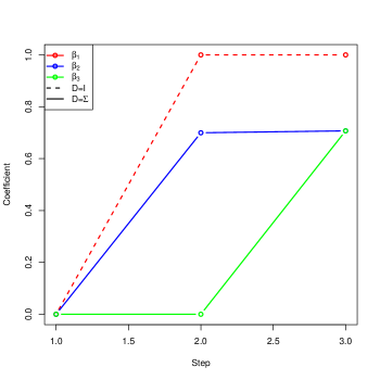
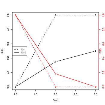
Figure 3.2: A toy example in which the sparsest solution has more uncertainty than the next sparsest one (see Section 2.2). Left: the regression coefficients at each stage of the FS algorithm. Only non-zero coefficients are plotted. Right: the uncertainty as estimated by $||S\boldsymbol{\beta}||_{2}$ (black), with residual sum of squares (RSS) on the right axis (red). The results are identical for lasso and LARS.

4 Application to biomass characterization data

In this section, we present results for both LARS and DS applied to a biomass characterization data set, with and without scaling. We highlight the challenges in working with this data, and illustrate the efficacy of scaling.

4.1 Description of the data

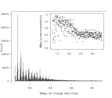
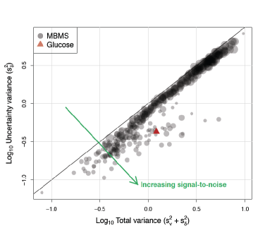
Figure 4.1: Graphical summary of the biomass characterization data. The top plot shows a typical raw MBMS spectrum. The inset shows, after pre-processing, the maximum cross-correlations for each peak and indicates a high degree of mutual dependence between the predictors. The bottom plot shows the distribution of variances estimated via a random one-way ANOVA model before normalization. The marker radius is proportional to mass-to-charge ratio of the peak, while the response ratio is indicated by a red triangle. A $1:1$ ratio is indicated by a black line. Points lying further down and to the right of the solid black line have higher fidelity (i.e., higher signal-to-noise ratio).

The characterization experiment we consider is motivated by a desire to quickly and inexpensively screen potential biofuel candidates for recalcitrance - a plant’s natural resistance to releasing usable sugars - after a chemical or enzymatic pre-treatment. Here, $n=759$ switchgrass plants were grown at different outdoor locations and in uncontrolled conditions. The predictors consist of $p=421$ pyrolysis molecular beam mass spectral (pyMBMS or MBMS, Sykes et al. (2009)) lines measured twice for each sample. As each sample is pyrolyzed, the spectrometer counts the number of molecules that reach a detector over a range of mass-to-charge ratios. The raw spectrum for each sample is then normalized to have unit mass and each peak is divided by a standard (control) value measured during the same run, allowing samples from different experiments to be compared directly. So, after pre-processing, each peak may be thought of as being an expression level for that mass-to-charge ratio relative to a control.

The response is the mass fraction of extractable glucose as inferred by the absorbance of 510-nm visible light, where each sample is measured in triplicate (Selig et al., 2011). In this experiment, a previously validated linear model is calibrated via measurement of a pure glucose sample. The mass and absorbance of each biological sample from the same run are then input to the calibrated model, yielding an estimate of glucose mass fraction for that sample.

The question we ask is: can the MBMS spectrum (a proxy for chemical composition) be used to predict the mass fraction of extractable glucose (usable biofuel)? To answer this, we seek a sparse linear model that incorporates estimates of uncertainty. Brief justifications for this approach are:

• Sparse: The spectroscopy experiment results in high cross-correlations between the peaks because large masses break into smaller ones in a somewhat predictable way. Hence, we expect a significant amount of redundancy in the peaks. In addition, the relationship between mass spectral peaks and cell chemistry is complex, making a sparse model appealing in that it narrows the focus of future investigations to a few, rather than hundreds, of peaks and their associated compounds.

• Incorporates uncertainty: Some of the peaks are far noisier than others, leading to unequal uncertainties. We would like to ensure that the model depends on the noisy peaks as little as possible, without completely excluding them from consideration.

• Linear: The assumed physical model is one of linear mixture, i.e., doubling the concentration of an analyte in the sample should result in a doubling of its spectral signature.

The data are summarized graphically in Figure 4.1. A typical raw mass spectrum is shown in the left panel where line height indicates count following convention for this field. The inset plot shows the maximum absolute cross-correlation of each peak with every other peak, from which we infer that there is a high degree of linear dependence among the variables, especially the smaller masses. In the right panel, the estimated total and within-sample ANOVA variances are shown before normalization or scaling, with equality indicated by a black line. The mass-to-charge ratios of the MBMS lines are proportional to the marker radius while glucose is indicated by a triangle. Clearly, many of the peaks are quite noisy, with almost all of the variance attributed to noise.

4.2 Methods

Model selection was performed using nested $k$-fold cross validation (CV), in which standard $k$-fold CV errors were averaged over $100/k$ outer loops for $k=2,5,$ and $10$. This approach ensured that $100$ different prediction models were validated for each choice of $k$. We fit both LARS and Dantzig models for comparison. LARS models were fit in ${\tt R}$ R F (2010) using the ${\tt lars}$ package (Hastie and Efron, 2011), and Dantzig in ${\tt MATLAB}$ using the ${\tt L_{1}\,\,Homotopy\,\,Toolbox}$ of Mat (2011); Asif and Romberg (2012, 2010). As has been suggested before (e.g., Elad (2010) Chapter 8.5), it can sometimes be beneficial to regress $\mathbf{y}$ on the sparse predictor set using another fitting procedure. For comparison, we used the LARS- and Dantzig-selected peaks as input to cross validated ridge regression via the ${\tt parcor}$ package in ${\tt R}$ (Kraemer and Schaefer, 2010). In all instances, the scaling matrix was estimated as part of the cross validation procedure (see Appendix for details).

4.3 Results

Cross-validation results are given in Table Cross validation procedure. in the Appendix, and may be summarized as follows. Scaling leads to:

1. improved accuracy, as measured by cross-validated MSEP, for both LARS and DS (Figure 4.2)

2. increased sparsity for both LARS and DS (Figure 4.3)

3. higher degree of consistency between LARS and DS

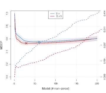
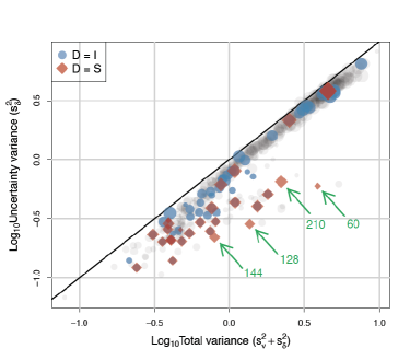
Figure 4.2: LARS cross validation results for $k=10$. The top plot shows the mean square error of prediction (MSEP) in bold lines and standard error as shaded regions. The dashed lines are estimates of uncertainty via $||S\hat{\boldsymbol{\beta}}||_{2}$, with units on the right axis. The optimal model is indicated with an x. Apparently, scaling by uncertainty variances leads to a sparser and more accurate model, with less associated uncertainty. The bottom plot is identical to the one in Figure 4.1, but with solution coordinates selected by LARS given different markers based on scaling (blue circles: unscaled, red diamonds: scaled). At least 4 peaks with high signal-to-noise are clearly selected after scaling that are not otherwise (green arrows, with numbers indicating the $m/z$ ratio).

The left panel of Figure 4.2 shows the prediction error per LARS step (solid lines), the standard error (shaded regions), and the uncertainty as estimated by $||S\hat{\boldsymbol{\beta}}||_{2}$ for $k=10$ (dashed lines). The optimal models are indicated by x’s. While the standard error of prediction is similar for the scaled and unscaled case, the uncertainty accumulates more slowly for the scaled input (almost identical results hold for $k=2,5$, not shown). The right panel provides a graphical impression of the quality of the variables selected for the scaled and unscaled data. One can see that, in general, the scaled approach (red diamonds) leads to selection of peaks with higher signal-to-noise ratio, indicated by green arrows, than the unscaled (blue circles).

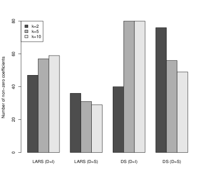
Figure 4.3: Number of non-zero coefficients for LARS and DS for $k=2,5,10$. In all cases, the prediction error decreases as $k$ (i.e., the number of training samples) increases. Without scaling, the more accurate models use more variables while with scaling, remarkably, they use fewer.

Figure 4.3 shows the sparsity of the LARS and DS models as a function of the CV fold sizes. Remarkably, the number of non-zero coefficients for both LARS and DS actually increases with increasing sample size when the data are unscaled. This is somewhat surprising since, heuristically, one would expect the model selection to be more discriminating as more samples are utilized. On the other hand, the number of non-zeros decreases with increasing sample size for the scaled data. To explain this, we speculate that when the data are unscaled, it is more likely for the algorithm to select variables that are either neutral or even detrimental with respect to prediction. If this is the case, then our results suggest that scaling leads to a more discriminating variable selection and higher prediction accuracy.

Finally, while the LARS and DS solutions are not in perfect agreement in either case (scaled or unscaled), they are seen to be in better agreement after scaling. Only $46\%$ of the LARS peaks are also selected by DS without scaling, while the number is $86\%$ with scaling. Alternatively, of the total number of distinct peaks selected by LARS and DS combined, only 24% are common to both without scaling, while 45% are common to both with scaling.

4.4 Discussion

It should be stated up front that the assumption of linearity made in Section 4.1 does not appear to be completely valid. While the assumption should be valid on physical grounds, there are obviously experimental, biological or other factors that introduce significant error terms beyond those formulated in Section 2.1. That said, the fact that scaling leads to a reduction in CV error, increased sparsity, and better agreement between LARS and DS suggests that the method can still be practically useful under non-ideal circumstances.

While some of the peaks identified by both scaled LARS and DS have been previously recognized as related to recalcitrance, many have not (see Table 2 in Appendix). Of particular interest are the peaks with large $m/z$ ratios, as these are less likely to be correlated coincidentally with recalcitrance: light particles can originate from a variety of sources, but less so for larger particles. Furthermore, some of the unknown peaks have regression coefficients that are not small. We believe that these results warrant taking a further look at the unknown peak associations to better understand chemical mechanisms of recalcitrance.

5 Conclusions

We have argued that sparse regression under design uncertainty presents several challenges that (to the best of our knowledge) have not been addressed in the literature. Focusing on the the uncertainty term, $||\Sigma\hat{\boldsymbol{\beta}}||_{2}^{2}$, in the residual error (2.2), we propose a scaling of the design variables by their uncertainty variances. In the context of greedy algorithms, doing this guarantees a uniform growth of uncertainty regardless of the order in which the variables are selected. Within the lasso formulation, scaling is shown to enforce an $l_{1}$ penalization of the uncertainty. In the Dantzig selector context, scaling leads to modified bounds on the residual error that reflect the amount of uncertainty associated with each variable.

In a biomass characterization application, scaling is shown empirically to reduce uncertainty in the optimal solution. It also leads to sparser solutions and lower prediction error. The solution estimates are improved even further if the LARS- and Dantzig-selected peaks are used independently for ridge regression. In addition, these models are more consistent with one another after scaling, that is, they identify more of the same predictors. The improvements resulting from scaling are promising and deserve further consideration.

Appendix

ANOVA model.

We use a one way, random effects ANOVA model to estimate the uncertainty variances. Let $r$ denote the number of replicate measurements of a random variable $Z$ and let $n$ denote the number of samples. The relevant quantities needed to estimate the variance components are shown in Table 1. In particular, the estimates are $s_{\delta}^{2}$ = SSE/df, and $s_{\nu}^{2}$ = (SSTr/df-$\sigma_{\delta}^{2}$)/$r$.

Source	df	Sum of squares	Expected mean square
Treatment	$n-1$	SSTr = $\sum_{i=1}^{n}r(\bar{z}_{i\cdot}-\bar{z}_{\cdot\cdot})^{2}$	$r\sigma_{\nu}^{2}+\sigma_{\delta}^{2}$
Error (uncertainty)	$n(r-1)$	SSE = $\sum_{i=1}^{n}\sum_{j=1}^{r}(z_{ij}-\bar{z}_{i\cdot})^{2}$	$\sigma_{\delta}^{2}$

Table 1: Standard one-way, random effects ANOVA table.

Cross validation procedure.

For clarity, we outline our procedure for cross-validated model selection using replicated measurements. It is a completely standard cross-validation procedure with the simple addition that we estimate the uncertainty variances only from the training data.

For each of the $k$ cross-validation groups:

1. Split the data into training, $\{\mathbf{y}_{train},X_{train}\}$, and test sets, $\{\mathbf{y}_{test},X_{test}\}$, of appropriate sizes.

2. Using only $X_{train}$, estimate the error variances, $s_{\delta_{j}}^{2}$, via a suitable method (we used one-way, random effects ANOVA).

3. Form the diagonal matrix $D_{jj}=s_{\delta_{j}}^{2}$ and scale the training data, $X_{train}\leftarrow X_{train}D^{-1}$.

4. Fit the desired models to $\mathbf{y}_{train}$ using scaled $X_{train}$.

5. Using $D$ from step 3, scale the test data, $X_{test}\leftarrow X_{test}D^{-1}$, and predict.

Model selection method	Scaling	$k$	# predictors	MSEP	Avg # predictors	Avg MSEP
		2	47	0.564
LARS	NO	5	57	0.551	54.3	0.555
		10	59	0.550
		2	36	0.539
LARS	YES	5	31	0.531	31.7	0.533
		10	28	0.530
		2	47	0.508
LARS-RR	NO	5	57	0.485	54.3	0.493
		10	59	0.485
		2	36	0.492
LARS-RR	YES	5	31	0.491	31.7	0.492
		10	28	0.494
		2	40	0.622
Dantzig selector	NO	5	80	0.583	66.7	0.599
		10	80	0.574
		2	76	0.547
Dantzig selector	YES	5	56	0.528	60.3	0.536
		10	49	0.523
		2	40	0.512
Dantzig-RR	NO	5	80	0.487	66.7	0.494
		10	80	0.482
		2	76	0.460
Dantzig-RR	YES	5	56	0.454	60.3	0.455
		10	49	0.451
		2	421	0.533
Ridge regression	NO	5	421	0.536	421	0.535
		10	421	0.535
		2	421	0.515
Ridge regression	YES	5	421	0.517	421	0.516
		10	421	0.517

Results of $k$-fold cross validation (see also Figure 4.3). The -RR suffix indicates ridge regression was performed on the subset selected by the corresponding sparse algorithm. For comparison, results for ridge regression using all of the predictor variables are also shown.

$m/z$	Assignment inSykes et al. (2008)	Avg. coefficient (relative to max)
45	?	+1.0000
60	C5 sugars	-0.0534
120	Vinylphenol	-0.2519
126	?	-0.1432
128	?	-0.0482
129	?	-0.2177
137	Ethylguaiacol, homovanillin, coniferyl alcohol	-0.7648
143	?	+0.1795
144	?	-0.2338
150	Vinylguaiacol	+0.8777
159	?	+0.1016
160	?	+0.1988
164	Allyl $\pm$ propenyl guaiacol	-0.3966
168	4-Methyl-2, 6-dimethoxyphenol	-0.3949
175	?	+0.0554
182	Syringaldehyde	-0.0734
194	4-Propenylsyringol	-0.8661
208	Sinapyl aldehyde	-0.0038
210	Sinapyl alcohol	+0.4334
226	?	+0.3021
264	?	+0.1883
287	?	-0.1646
371	?	-0.1970
374	?	+0.2153

Table 2: Peaks identified by both scaled LARS and DS for $k=10$. The peaks previously identified in Sykes et al. (2008) as significant to sugar release are described where possible. The LARS and DS regression coefficients were averaged and divided by the maximum to highlight the relative significance and sign of correlation of the peaks. Some of the most highly-weighted variables have not previously been identified as being related to recalcitrance.

References

- Asif and Romberg [2009] M. Salman Asif and Justin Romberg. Dantzig selector homotopy with dynamic measurements. Proceedings of the SPIE, 7246, 2009.
- Asif and Romberg [2010] M. Salman Asif and Justin Romberg. Dynamic updating for l1 minimization. IEEE Journal of Selected Topics in Signal Processing, 4(2):421–434, 2010.
- Asif and Romberg [2012] M. Salman Asif and Justin Romberg. L1 homotopy: a MATLAB Toolbox for homotopy algorithms in l1 norm minimization problems, 2012. URL http://users.ece.gatech.edu/ sasif/homotopy/.
- Bickel et al. [2009] Peter J. Bickel, Ya’acov Ritov, and Alexandre B. Tsybakov. Simultaneous analysis of lasso and dantzig selector. Annals of Statistics, 37(4):1705–1732, 2009.
- Candes and Tao [2007] Emmanuel Candes and Terence Tao. The dantzig selector: statistical estimation when p is much larger than n. Annals of Statistics, 35(6):2313–2351, 2007.
- Chen et al. [1998] Scott Shaobing Chen, David L. Donoho, and Michael A. Saunders. Atomic decomposition by basis pursuit. SIAM Journal on Scientific Computing, 20(1):33–61, 1998.
- Chen et al. [2001] Scott Shaobing Chen, David L. Donoho, and Michael A. Saunders. Atomic decomposition by basis pursuit. SIAM Review, 43(1):129–159, 2001.
- Donoho and Tsaig [2008] David L. Donoho and Yaakov Tsaig. Fast solution of l1-norm minimization problems when the solution may be sparse. IEEE Transactions on Information Theory, 54(11):4789–4812, 2008.
- Efron et al. [2004] Bradley Efron, Trevor Hastie, Iain Johnstone, and Robert Tibshirani. Least angle regression. The Annals of Statistics, 32(2):407–499, 2004.
- Elad [2010] Michael Elad. Sparse and redundant representations. Springer, 2010.
- Fuller [1987] Wayne A. Fuller. Measurement error models. John Wiley and Sons Ltd., 1987.
- Fuller [1995] Wayne A. Fuller. Estimation in the presence of measurement error. International Statistical Review, 63(2):121–141, August 1995.
- Gillard [2010] Jonathan Gillard. An overview of linear structural models in errors in variables regression. Revstat Statistical Journal, 8(1):57–80, 2010.
- Golub and Loan [1980] Gene H. Golub and Charles F. Van Loan. An analysis of the total least squares problem. SIAM Journal of Numerical Analysis, 17(6):883–893, 1980.
- Hastie and Efron [2011] Trevor Hastie and Brad Efron. lars: Least Angle Regression, Lasso and Forward Stagewise, 2011. URL http://CRAN.R-project.org/package=lars.
- Hastie et al. [2007] Trevor Hastie, Jonathan Taylor, Robert Tibshirani, and Guenther Walther. Forward stagewise regression and the monotone lasso. Electronic Journal of Statistics, 1:1–29, 2007.
- Huang et al. [2008] Jian Huang, Shuangge Ma, and Cun-Hui Zhang. Adaptive lasso for sparse high-dimensional regression models. Statistica Sinica, 18:1603–1618, 2008.
- Kraemer and Schaefer [2010] Nicole Kraemer and Juliane Schaefer. parcor: regularized estimation of partial correlation matrices, 2010. URL http://CRAN.R-project.org/package=parcor.
- Mat [2011] Matlab version 7.12.0 (R2011a). The MathWorks Inc., Natick, Massachusetts, 2011.
- Percival et al. [2011] Daniel Percival, Kathryn Roeder, Roni Rosenfeld, and Larry Wasserman. Structured, sparse regression with application to hiv drug resistance. The Annals of Applied Statistics, 5(2A):628–644, 2011.
- R F [2010] R: A Language and Environment for Statistical Computing. R Foundation for Statistical Computing, Vienna, Austria, 2010. URL http://www.R-project.org/.
- Rosenbaum and Tsybakov [2010] Mathieu Rosenbaum and Alexandre B. Tsybakov. Sparse recovery under matrix uncertainty. The Annals of Statistics, 38(5):2620–2651, 2010.
- Selig et al. [2011] Michael J. Selig, Melvin P. Tucker, Cody Law, Crissa Doeppke, Michael E. Himmel, and Stephen R. Decker. High throughput determination of glucan and xylan fractions in lignocellulose. Biotechnology Letters, 33:961–967, 2011.
- Sun and Zhang [2011] Tingni Sun and Cun-Hui Zhang. Scaled sparse linear regression. arXiv:1104.4595v2 [stat.ML], April 2011. URL http://arxiv.org/abs/1104.4595.
- Sykes et al. [2008] Robert Sykes, Bob Kodrzycki, Gerald Tuskan, Kirk Foutz, and Mark Davis. Within tree variability of lignin composition in populus. Wood Science and Technology, 42:649–661, 2008.
- Sykes et al. [2009] Robert Sykes, Matthew Yung, Evandro Novaes, Matias Kirst, Gary Peter, and Mark Davis. High-throughput screening of plant cell-wall composition using pyrolysis molecular beam mass spectroscopy. Methods in Molecular Biology, 581:169–183, 2009.
- Tibshirani [1996] Robert Tibshirani. Shrinkage and selection via the lasso. Journal of the Royal Statistical Society: Series B (Methodological), 58(1):267–288, 1996.
- Tibshirani and Taylor [2011] Ryan J. Tibshirani and Jonathan Taylor. The solution path of the generalized lasso. The Annals of Statistics, 39(2):1335–1371, 2011.
- Tropp [2004] Joel A. Tropp. Greed is good: algorithmic results for sparse approximation. IEEE Transactions on Information Theory, 50(10):2231–2242, 2004.
- Wagener and Dette [2011a] Jens Wagener and Holger Dette. The adaptive lasso in high dimensional sparse heteroscedastic models. Discussion paper, Ruhr-Unversitat Bochum, Bochum, Germany, 2011a.
- Wagener and Dette [2011b] Jens Wagener and Holger Dette. Bridge estimators and the adaptive lasso under heteroscedasticity. Technical report, Ruhr-Unversitat Bochum, 2011b.
- Yuan and Lin [2006] Ming Yuan and Yi Lin. Model selection and estimation in regression with grouped variables. Journal of the Royal Statistical Society: Series B (Methodological), 68:49–67, 2006.
- Zhu et al. [2011] Hao Zhu, Geert Leus, and Georgios B. Giannakis. Sparsity-cognizant total least squares for perturbed compressive sampling. IEEE Transactions on Signal Processing, 59(5):2002–2016, May 2011.
- Zou and Hastie [2005] Hui Zou and Trevor Hastie. Regularization and variable selection via the elastic net. Journal of the Royal Statistical Society: Series B (Methodological), 67:301–320, 2005.