Long-range adiabatic quantum state transfer through tight-binding chain as quantum data bus

Abstract

We introduce a scheme based on adiabatic passage which allows for long-range quantum communication through tight-binding chain with always-on interaction. By adiabatically varying the external gate voltage applied on the system, the electron can be transported from the sender’s dot to the aim one. We numerically solve the schrödinger equation for a system with given number of quantum dots. It is shown that this scheme is a simple and efficient protocol to coherently manipulate the population transfer under suitable gate pulses. The dependence of the energy gap and the transfer time on system parameters is analyzed and shown numerically. Our method provides a guidance for future realization of adiabatic quantum state transfer in experiments.

I Introduction

Quantum state transfer (QST), as the name suggests, refers to the transfer of an arbitrary quantum state from one qubit to another, which is a central task in quantum information science. For the solid-state based quantum computing at the large scale, it is very crucial to have a solid system serving as such quantum data bus, which can provide us with a quantum channel for quantum communication. During the last years many efforts have been made in different fields to design a feasible proposal for perfect QST. One kind of proper QST proposals is based on solid-state system with always-on interaction Bose1 ; Song ; Christandle1 . The communication is achieved by simply placing a quantum state at one end of the chain and waiting for an optimized time to let this state propagate to the other end with a high fidelity. The other kinds of proposals have paid much attention to adiabatic passage for coherent QST in time-evolving quantum systems, which is a powerful tool for manipulating a quantum system from an initial state to a target state. This way of population transfer has the important property of being robust against small variations of the Hamiltonian and the transport time, which is crucial in experiment since the system parameters are often hard to control. The typical scheme for coherently spatial population transfer has been independently proposed for neutral atoms in optical traps Eckert and for electrons in quantum dot (QD) systems CTAP via a dark state of the system, which is termed coherent tunneling via adiabatic passage (CTAP) following Ref. CTAP . In such a scheme, the tunneling interaction between adjacent quantum units is dynamically tuned by changing either the distance or the height of the neighboring potential wells following a counterintuitive scheme which is a solid-state analog of the well-known stimulated Raman adiabatic passage (STIRAP) protocol STIRAP of quantum optics. Since then, the CTAP technique has been proposed in a variety of physical systems for transporting single atoms atom1 ; atom2 , spin states spin , electrons electron1 ; electron2 and Bose-Einstein condensates BEC1 ; BEC2 ; BEC3 . It has also been considered as a crucial element in the scale up to large quantum processors LR1 ; LR2 .

Recently, Ref. chen1 presented a scheme to adiabatically transfer an electron from the left end to the right end of a three dot chain using the ground state of the system. This technique is a copy of the frequency chirping method CF1 ; CF2 , which is used in quantum optics to transfer the population of a three-level atom of the Lambda configuration. The scheme chen1 is presented as an alternative to a well known transfer scheme (CTAP) CTAP . However, different from CTAP process, the protocol in Ref. chen1 considers a three QD array with always-on interaction which can be manipulated by the external gate voltage applied on the two external dots (sender and receiver). Through maintaining the system in the ground state, it shows that it is a high-fidelity process for a proper choice of system parameters and also robust against experimental parameter variations. The obvious extension of this work is to consider the passage through more than one intervening dot chen2 . In this paper we will consider a quasi-one-dimensional chain of QDs, which is schematically illustrated in Fig. 1. The central tight-binding chain serves as the quantum channel and two external QDs are attached to the media chain. The sender (Alice) and the receiver (Bob) control one external QD each and Alice transmits information via a qubit using the chain to Bob by adiabatically changing the gate voltages. Different from previously discussed schemes, we will consider a fixed $N$-site coupled QDs media chain and QST can be realized in required transfer distance by modulating the positions where QD A and B are connected to the chain. In particular, the nearest-neighbor hopping amplitudes are set to be uniform. We first theoretically elaborate the adiabatic QST in this scheme. Taking a 50-dot structure as an example, we show that the electron can be robustly transported from Alice to Bob through the media chain, by slowly varying the gate voltages.

The paper is organized as follows. In Sec. II the model is setup and we describe the adiabatic transfer of an electron between QDs. In Sec. III we show numerical results that substantiate the analytical results. The last section is the summary and discussion of the paper.

II Model Setup

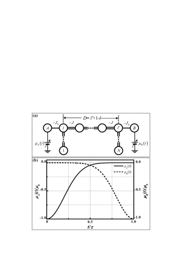
Figure 1: (a) Schematic illustrations of adiabatic QST in multi-dot array. The system is controlled by external gates voltage $\mu_{i}(t)$ $(i=A,$ $B)$. By adiabatically varying the gates voltage, one can achieve long-range QST from the QD $A$ to QD $B$ of the chain. (b) Gate voltages as a function of time (in units of $\tau$). $\mu_{A}(t)$ is the solid line and $\mu_{B}(t)$ is the dash line.

Consider a quasi-one-dimensional chain of QDs, realized by the empty or singly occupied states of a positional eigenstate, see Fig. 1. The whole quantum system consists of two sites ($A$ and $B$) and a simple tight-binding $N$-site chain. The sender (Alice) and the receiver (Bob) can only control the external gates voltage $\mu_{\alpha}(t)$ $(\alpha=A,$ $B)$. The total Hamiltonian $\mathcal{H}(t)=\mathcal{H}_{M}+\mathcal{H}_{I}+\mathcal{H}_{C},$contains three parts, the medium Hamiltonian

$$\mathcal{H}_{M}=-J\sum_{j=1}^{N-1}\left|j\right\rangle\left\langle j+1\right|+\text{h.c.}$$ (1)

describing the tight-binding chain with uniform nearest neighbor hopping integral $-J$ $(J>0),$ the coupling Hamiltonian

$$\mathcal{H}_{I}=-J_{0}\left(\left|A\right\rangle\left\langle l\right|+\left|B\right\rangle\left\langle l^{\prime}\right|\right)+\text{h.c.},$$ (2)

describing the connections between QDs $A$, $B$, and the chain with hopping integral $-J_{0}$ $(J_{0}>0)$, and the operating Hamiltonian

$$\mathcal{H}_{C}=\mu_{A}(t)\left|A\right\rangle\left\langle A\right|+\mu_{B}(t)\left|B\right\rangle\left\langle B\right|$$ (3)

describing the adiabatic manipulation of the Hamiltonian parameters. In $\mathcal{H}(t)$, $\left|j\right\rangle$ represents the Wannier state localized in the $j$-th quantum site for $j=A,$ $1,$ $2,...,$ $N,$ $B$. In $\mathcal{H}_{I}$, $l$ and $l^{\prime}$ denote the sites of medium connecting to the QDs $A$ and $B$. The distance between $A$ and $B$ is $D=l^{\prime}+1-l$. In this proposal, we just consider one connection way: $l^{\prime}=N+1-l$, that is the quantum state is transferred between site $A$ and its mirror-conjugate site $B$. In term $\mathcal{H}_{C}$, $\mu_{A}(t)$ and $\mu_{B}(t)$ are site energies (externally controlled), which are modulated by a Gaussian pulses (shown in Fig. 1(b))

$$\mu_{A}(t) = -\mu_{0}\exp\left[-\frac{1}{2}\alpha^{2}t^{2}\right],$$

$$\mu_{B}(t) = -\mu_{0}\exp\left[-\frac{1}{2}\alpha^{2}\left(t-\tau\right)^{2}\right],$$ (4)

where $\mu_{0}$ is the peak voltage of the pulse; $\tau$ and $\alpha$ the total adiabatic evolution time and standard deviation of the control pulse. To realize high fidelity transfer in this scheme, the peak voltage $\mu_{0}$ must be much larger than hopping integral, i.e. $\mu_{0}\gg J,J_{0}$. The reason is that small peak values improve adiabaticity, but lead to a low fidelity because the final instantaneous eigenstate is not the desired one. According to Ref. chen2 , the transfer is optimized when we choose $\alpha=8/\tau$. Throughout this paper, all energies ($J_{0}$ and $\mu_{0}$) are scaled in units of $J$, and evolution time $\tau$ is in units of $1/J$.

In this proposal, we focus our study on the ground state $\left|\psi_{g}(t)\right\rangle$ of Hamiltonian $\mathcal{H}(t)$ to induce population transfer from state $\left|A\right\rangle$ to $\left|B\right\rangle$. For single electron transfer, a state in the single particle Hilbert space is assumed as $\left|\psi_{k}\right\rangle=f_{A}^{k}\left|A\right\rangle+\sum_{j=1}^{N}f_{j}^{k}\left|j\right\rangle+f_{B}^{k}\left|B\right\rangle$, where $k$ denotes the momentum. Duo to the translational symmetry of the present system, the instantaneous Hamiltonian’s eigen equation for $f_{j}^{k},$ $j\in\left[1,N\right]$ is easily shown to be

$$-J\left[f_{j-1}^{k}+f_{j+1}^{k}\right] = \left[\varepsilon_{k}-V_{A}\left(\varepsilon_{k}\right)\delta_{j,l}-V_{B}\left(\varepsilon_{k}\right)\delta_{j,N+1-l}\right]f_{j}^{k},$$

$$J_{0}f_{A}^{k} = V_{A}\left(\varepsilon_{k}\right)f_{l}^{k},$$ (5)

$$J_{0}f_{B}^{k} = V_{B}\left(\varepsilon_{k}\right)f_{N+1-l}^{k},$$

here $\varepsilon_{k}$ is the eigenenergy and the term

$$V_{i}\left(\varepsilon_{k}\right)=\frac{J_{0}^{2}}{\varepsilon_{k}+\mu_{i}},i\in\left[A,B\right]$$ (6)

on the right hand side is contributed by the interactions between the sites $A$, $B$, and medium chain which is dependent on the eigenenergy $\varepsilon_{k}$. The $\delta$-type potential forms a confining barrier to the transportation of single electron in the chain and forms a bounded state of single electron, similar to those proposed in Ref. Sun . In this work, we focus our attention on the bound state, which is the ground state of the total system to realize the long-range QST.

Starting from $t=0$, we have $\mu_{A}(0)=-\mu_{0}$ and $\mu_{B}(0)\approx 0$. The solution to Eq. (5) is

$$\left|\psi_{g}(0)\right\rangle=\mathcal{N}^{-1/2}\left[\sum_{j=1}^{N}e^{-\kappa\left|j-l\right|}\left|j\right\rangle+\frac{\lambda_{+}}{J_{0}}\left|A\right\rangle+\frac{\lambda_{-}}{J_{0}}e^{-\kappa(N+1-2l)}\left|B\right\rangle\right],$$ (7)

where $\lambda_{\pm}=\left(\sqrt{\mu_{0}^{2}+4J_{0}^{2}}\pm\mu_{0}\right)/2$ and $\kappa=\ln\left(\lambda_{+}/J\right)$; $\mathcal{N}=\sum_{j=1}^{N}e^{-2\kappa\left|j-l\right|}+\left(\mu_{0}^{2}+2J_{0}^{2}\right)/J_{0}^{2}$ is the normalization factor. By choosing a sufficiently large value of $\mu_{0}$, the ground state $\left|\psi_{g}(0)\right\rangle$ can be reduced to $\left|\psi_{g}(0)\right\rangle\approx\left|A\right\rangle$.

With the same results, in the time limit $t=\tau$, the parameter $\mu_{A}(t)$ goes to zero and $\mu_{B}(t)$ goes to $-\mu_{0}$. Duo to the reflection symmetry (relabeling sites from right to left) of the system, for $j=A,1,2,...,N,B,$

$$\langle j\left|\psi_{g}(\tau)\right\rangle=\langle\bar{j}\left|\psi_{g}(0)\right\rangle.$$ (8)

We have used $\bar{j}=N+1-j$ to indicate the mirror-conjugate site of $j$. This leads to the final ground state $\left|\psi_{g}(\tau)\right\rangle\approx\left|B\right\rangle$. To illustrate with an example, the probability of $\left|B\right\rangle$ in $\left|\psi_{g}(\tau)\right\rangle$ can achieve 99.7% when the parameters are set to be $J_{0}/J=1$ and $\mu_{0}/J=20$. Preparing the system in state $\left|\Psi\left(t=0\right)\right\rangle=\left|A\right\rangle\,$and adiabatially changing $\mu_{A}(t)$ and $\mu_{B}(t)$, one can see that the system will end up in $\left|B\right\rangle$,

$$\left|\Psi\left(t=0\right)\right\rangle=\left|A\right\rangle\rightarrow\left|\Psi\left(t=\tau\right)\right\rangle=\left|B\right\rangle,$$ (9)

hence we can see that a high fidelity transfer may still be possible, even with imperfect controls.

In the absence of hopping term between the two external QDs $A$, $B$ and the medium chain ($J_{0}=0$), the Hamiltonian $\mathcal{H}(t)$ can be diagonalized as

$$\mathcal{H}(t)=\sum_{k}-2J\cos k\left|k\right\rangle\left\langle k\right|+\mu_{A}(t)\left|A\right\rangle\left\langle A\right|+\mu_{B}(t)\left|B\right\rangle\left\langle B\right|$$

with $\left|k\right\rangle=\sqrt{2/\left(N+1\right)}\sin(kj)\left|j\right\rangle$, where $k=n\pi/(N+1),n=1,2,...,N$. One can see that at $t=\tau/2$, the eigenstates $\left|A\right\rangle$ and $\left|B\right\rangle$ are degenerate which leads to a breakdown of adiabaticity. The presence of the hopping term $J_{0}$ will open up energy gap at the crossing. To evaluate instantaneous eigenvalues of the Hamiltonian is generally only possible numerically. In Fig. 2(a) we present the results showing the eigenenergy gap between the instantaneous first-excited state and ground state undergoing evolution due to modulation of the gate voltages according to pulse Eq. (4). The eigenvalues shown in this figure exhibit pronounced avoided crossing and approach nonzero minimum $\Delta=\varepsilon_{1}\left(\tau/2\right)-\varepsilon_{g}\left(\tau/2\right)$. This minimum energy gap plays a significant role in the transfer, because the total evolution time should be larger enough compared to $\Delta$. In this scheme, the energy gap $\Delta$ depends both on the transfer distance $D$ and the coupling constance $J_{0}$. To study the relationship between the total evolution time and system parameters is one of the important contributions of this paper.

As an example, we show in Fig. 2 the effect two factors has on the energy gap $\Delta$ for a system with $N=48$ QDs and coupling strength $J=1.0$. The pulse’s parameters we choose are $\alpha=8/\tau$, and $\mu_{0}=20$. In Fig. 2(b), we plot the energy gap $\Delta$ as a function of transfer distance $D$ for $J_{0}=0.5J$, and $J_{0}=0.7J$. The horizontal line $\delta\approx 3J\pi^{2}/N^{2}$ indicates the minimum gap of medium chain $\mathcal{H}_{M}$. One can see that the logarithmic scales chosen suggest that as transfer distance $D$ increasing there is an exponential disappearance of the gap $\Delta$. The smaller hopping constant $J_{0}$, the slower the decay of $\Delta$. The other thing is that $\Delta$ is also determined by the coupling strength $J_{0}$. Fig. 2(c) shows the numerically computed behavior of $\Delta$ as a function of $J_{0}$ for $D=8$, $16$, and $24$. As $J_{0}$ increases, the gap $\Delta$ increase for short-distance transfer ($D<N/3$) and decreases for long-distance transfer ($D>N/3$). The results shown in Fig. 2(c) also suggest that decreasing coupling strength $J_{0}$ can obtain relatively large $\Delta$ for long-range transfer. But it does not mean the weaker the coupling $J_{0}$, the better the result of QST will be. The reason is that the energy gap is not the sufficient and necessary condition for adiabatic process. In this proposal, the negative effects of distance on the gap can be partially compensated by $J_{0}$.

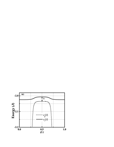
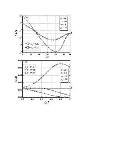
Figure 2: (a) The instantaneous eigenenergy (in units of $J$) of the lowest two states $\psi_{g}$ and $\psi_{1}$ through the gate pulse shown in Fig. 1(b). The gap is minimum at $t=\tau/2$, $\Delta=\varepsilon_{1}\left(\tau/2\right)-\varepsilon_{g}\left(\tau/2\right)$. (b) Plot of gap $\Delta$ (in units of $J$) as a function of transfer distance $D$ for $J_{0}=$0.5$J$, and 0.7$J$. The energy gap $\Delta$ is exponentially decreasing as transfer distance $D$ increase for a given $J_{0}$. (c) The gap $\Delta$ (in units of $J$) as a function of coupling constant $J_{0}$ for the transfer distance $D=$8, 16, and 24. The horizontal line $\delta$ is the minimum gap of the medium chain $\mathcal{H}_{M}$.

III Numerical Simulations

In this section let us firstly review the transfer process of this protocol. At $t=0$ we initialize the device so that the electron occupies site-$1$, i.e., the total initial state is $\left|A\right\rangle$. Provided we transform the gate pulses adiabatically, then the adiabatic theorem states that the system will stay in the same eigenstate. Therefore, the quantum state starting in $\left|A\right\rangle$ will end up in $\left|B\right\rangle$.

The analysis above is based on the assumption that the adiabaticity is satisfied. The adiabaticity parameter defined for this scheme is

$$\mathcal{A}\left(t\right)=\frac{\left|\left\langle\psi_{g}(t)\right|\partial\mathcal{H}/\partial t\left|\psi_{1}(t\right\rangle\right|}{\left|\varepsilon_{g}(t)-\varepsilon_{1}(t)\right|^{2}},$$ (10)

where $\left|\psi_{g}(t\right\rangle$ ($\left|\psi_{1}(t\right\rangle$) is the instantaneous ground state (first-excited state) of the Hamiltionian $\mathcal{H}(t)$ and $\varepsilon_{g}(t)$ ($\varepsilon_{1}(t)$) is the corresponding instantaneous eigenvalue of the state $\left|\psi_{g}(t\right\rangle$ ($\left|\psi_{1}(t\right\rangle$). For adiabatic evolution of the system we require $\mathcal{A}\left(t\right)\ll 1$ for all time, which greatly suppresses the quantum transition from the ground state $\left|\psi_{g}(t)\right\rangle$ to the first-excited state $\left|\psi_{1}(t)\right\rangle$. Fig. 3(a) and (b) show the numerical result of energy difference $\varepsilon_{1}(t)-\varepsilon_{g}(t)$ and $\mathcal{A}\left(t\right)\tau$ as a function of pulse time. Note that the appearance time of maxima of $\mathcal{A}\left(t\right)$ is not at the middle of the pulse sequence, but the energy difference $\varepsilon_{1}(t)-\varepsilon_{g}(t)$ at this time is slightly larger than the minimum gap $\Delta$. So we can use minimum gap $\Delta$ to estimate the minimum pulse time required for high-fidelity transfer. Fig. 3(c) shows the maximum adiabaticity $\max\{\mathcal{A}\left(t\right)\tau\}$ through the protocol as a function of $J_{0}$ for $D=10$, $16$, and $20$. One sees that there is an optimal value of $J_{0}$ which ensures the shortest time for realizing perfect QST and the optimal value decreases as transfer distance $D$ increases. To sum up, the adiabatic regime necessary to obtain transport with high fidelity can be concluded to the condition $\tau\gg 1/\Delta^{\ast}\left(D\right)$, where $\Delta^{\ast}\left(D\right)$ is the minimum gap of the system when the coupling strength $J_{0}$ takes the optimal value corresponding to transfer distance $D$.

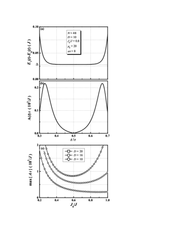
Figure 3: (a) The energy difference $E_{1}(t)-E_{g}(t)$ (in units of $J$) and (b) adiabaticity $\mathcal{A}\left(t\right)\tau$ (in units of $10^{3}/J$) as a function of time in the time interval $t\in[0.3\tau,0.7\tau]$. Note that the energy gap approximately equals $\Delta$ in a wide time range and the maxima of adiabaticity is not at the middle of the pulse sequence. (c) Maximum adiabaticity $\max\{\mathcal{A}\left(t\right)\tau\}$ through the protocol as a function of $J_{0}$ for three different transfer distances. $\max\{\mathcal{A}\left(t\right)\tau\}$ varies with $J_{0}$, and reaches minimum value when the $J_{0}$ takes specific value.

The consequent time evolution of the state is given by the Schrödinger equation (assuming $\hbar=1$)

$$i\frac{d}{dt}\left|\Psi\left(t\right)\right\rangle=\mathcal{H}(t)\left|\Psi\left(t\right)\right\rangle.$$ (11)

The time evolution creates a coherent superposition:

$$\left|\Psi\left(t\right)\right\rangle=c_{A}(t)\left|A\right\rangle+\sum_{j=1}^{N}c_{j}(t)\left|j\right\rangle+c_{B}(t)\left|B\right\rangle,$$ (12)

where $c_{j}(t)$ denotes the time-dependent probability amplitude for the electron to be in $j$-th QD. We define the probability of finding the electron on the medium chain as $\left|c_{M}(t)\right|^{2}=\sum_{j=1}^{N}\left|c_{j}(t)\right|^{2}$ that obeys the normalization condition$\,\left|c_{A}(t)\right|^{2}+\left|c_{M}(t)\right|^{2}+\left|c_{B}(t)\right|^{2}=1$. At time $\tau$ the fidelity of initial state transferring to the dot-$B$ is defined as $F=\left|\langle B\left|\Psi(\tau)\right\rangle\right|^{2}=\left|c_{B}(\tau)\right|^{2}$.

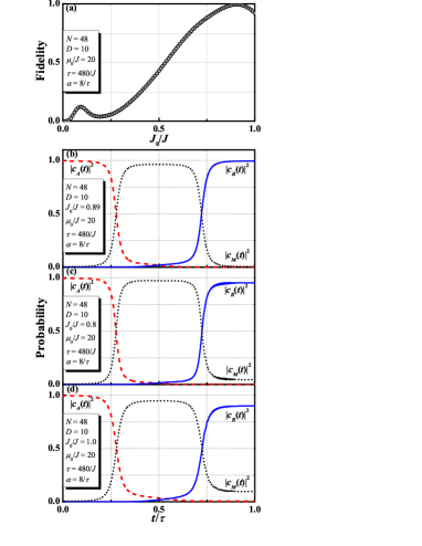
Figure 4: (Color online) QST from QD $A$ to $B$ attached to a tight-binding chain of length with $N=48$ for two different transfer distance: $D=11$ (a)-(d) and $D=21$ (e)-(h). (a) The transfer fidelity as a function of coupling strength $J_{0}$ for transfer distance $D=11$. The calculation was done for various values of $J_{0}$ at fixed total evolution time $\tau=480/J$. Note that there is an optimal value of $J_{0}$ to achieve high fidelity QST. Population transfer as a function of time obtained for three coupling strength $J_{0}$:(b) $J_{0}=0.8J$; (c) $J_{0}=0.91J$; (d) $J_{0}=1.0J$. Initially the population is on QD $A$ (dashed red line) and finally mainly on QD $B$ (solid blue line). The population on the media chain is shown as a dotted black line. (e) The same as in (a), but for transfer distance $D=21$ and $\tau=1200/J$. (f)-(h) The population behavior under the influence of $J_{0}$. The parameters are like that in (b)-(d).

In order to proceed, we used standard numerical methods to integrate the Schrödinger equation for probability amplitudes. Because the scheme relies on maintaining adiabatic conditions, we examine the effect of system parameters on the target state population. In Fig. 4, we consider the system with $N=48$ and show QST from QD $A$ to QD $B$ for two different transfer distance: $D=11$ and $D=21$. Firstly, we examine the effect of coupling strength $J_{0}$ on transfer fidelity. It is seen that there is an optimal value of $J_{0}$ to achieve high-fidelity transfer.

To illustrate the process of QST for $D=11$, we exhibit in Fig. 4(b)-(d) the exact evolution of the probabilities of finding electron in QD $A$ (red dashed line), $B$ (blue solid line), and media chain (black dotted line) as a function of time for three different values of coupling strength $J_{0}$ but the same remaining parameters ($\mu_{0}=20J$, $\tau=480/J$ and $\alpha=8/\tau$). We get good results for the transfer if we choose $J_{0}=0.89J$ as shown in Fig. 4(b). The populations on the QD $A$ and QD $B$ are exchanged in the expected adiabatic manner. If we choose parameters deviated from the optimum value, $J_{0}=0.8J$ and $1.0J$, we find the results in Fig. 4(c) and Fig.  4(d). We can see that a slight deviations from the values will breaks adiabaticity and lead to major deteriorations of the quality of transfer. When the transfer distance becomes large, we should enlarge evolution time $\tau$ to enhance the adiabaticity. In Fig. 4(e), transfer fidelity as a function of $J_{0}$ for transfer distance $D=21$ and evolution time $\tau=1200/J$. The time evolution of the probabilities the same as Fig. 4(b)-(d) for $D=21$ and three different $J_{0}$ are illustrated in Fig. 4(f)-(g). We can still see from Fig. 2 that the optimum value of $J_{0}$ to achieve high-fidelity transfer decreases as the transfer distance increase which is consistent with the results shown before.

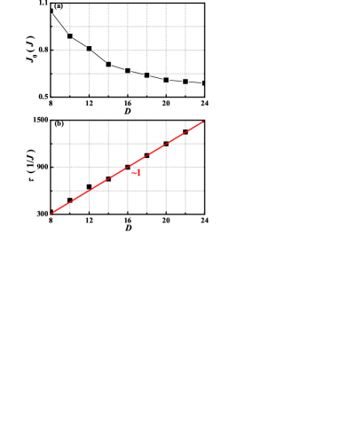
Figure 5: (Color online) For a given chain length $N=48$ and a chosen fidelity $F=0.995$, (a) the optimum value of coupling strength $J_{0}$ (in units of $J$) and (b) the minimum time $\tau$ (in units of $1/J$) required for state transfer varies as a function of transfer distance $D$. The other system parameters we choose is $J=1$, $\mu_{0}=20$ and $\alpha=8/\tau$. It shows that optimum value of $J_{0}$ decreases as $D$ increasing and time $\tau$ scales linearly with transfer distance $D$.

In order to provide the most economical choice of parameters for reaching high transfer efficiency, we perform numerical analysis, as shown in Fig. 5. Specifically, we depict the optimum coupling $J_{0}$ (shown in Fig. 5(a)) and the corresponding minimum state transfer time $\tau$ (shown in Fig. 5(b)) for a given chain length $N=48$ and a given tolerable transfer fidelity $F=99.5\%$, the minimum time varies as a function of transfer distance $D$. One can see that the time $\tau$ required for high-fidelity transfer scales linearly with transfer distance $D$.

IV Summary and Discussion

An efficient QST scheme should not only admit a state transfer of any quantum state in a fixed period of time of the state evolution with high fidelity, but also the transfer time can not grow fast as communication distance increases. In this paper, we have introduced a long-range transport mechanism for quantum information around a quasi-one-dimensional QDs network, based on adiabatic passage. This scheme is realized by modulation of gate voltages applied on the two external QDs which is connected to the tight-binding chain. Under suitable system parameters, the electron can be transported from the sender QD to the receiver one with high efficiency, carrying along with it the quantum information encoded in its spin. Different from the CTAPn Scheme CTAPn , our method is to induce population transfer through tight-binding chain by maintaining the system in its ground state and this is more operable in experiments. We have studied the adiabatic QST through the system by theoretical analysis and numerical simulations of the ground state evolution of tight-binding model. The result demonstrates that it is an efficient high-fidelity process (99.5%) for an economical choice of system parameters. Increasing the transfer distance, we found that the efficiency of QST is inversely proportional to the distance of the two QDs.

In a real system, decoherence is the main obstacle to the experimental implementation of quantum information Ivanov ; Kam . There are two sources of quantum decoherence in QDs, one is due to charge dephasing brought by lead-QD coupling and the other is due to the hyperfine interaction. For the former, the coherence time of quantum dot is $\sim$1 ns, which plays a role in this case. On the other hand, the maximum time in $N=48$ QD system needed for the appearance of the better fidelity is roughly proportional to $10^{4}/J$. As a simple estimate of the effects of decoherence, we compare this time with the dephasing time, which leads to a limit of coupling strength of $J$ of $\sim$10 THz. The probability of realization of this idea in experiment can be maximized by more precise manipulation technology and by cooling the system. Furthermore, the development of cold atom physics provides us with an alternative realization of our systems in experiment, because decoherence in cold-atom system is much less destructive.

References

- (1) S. Bose, Phys. Rev. lett. 91, 207901 (2003).
- (2) Z. Song and C. P. Sun, Low Temperature Physics 31, 686 (2005).
- (3) M. Christandl, N. Datta, A. Ekert and A.J. Landahl, Phys. Rev. Lett. 92, 187902 (2004).
- (4) K. Eckert, M. Lewenstein, R. Corbalán, G. Birkl, W. Ertmer, and J. Mompart, Phys. Rev. A 70, 023606 (2004).
- (5) A. D. Greentree, J. H. Cole, A. R. Hamilton, and L. C. L. Hollenberg, Phys. Rev. B 70, 235317 (2004).
- (6) N. V. Vitanov, T. Halfmann, B. W. Shore, and K. Bergmann, Annu. Rev. Phys. Chem. 52, 763 (2001).
- (7) K. Eckert, J. Mompart, R. Corbalan, M. Lewenstein, and G. Birkl, Opt. Commun. 264, 264 (2006).
- (8) T. Opatrný, K. K. Das, Phys. Rev. A 79, 012113 (2009).
- (9) T. Ohshima, A. Ekert, D. K. L. Oi, D. Kaslizowski, L. C. Kwek, e-print arXiv:quant-ph/0702019.
- (10) P. Zhang, Q. K. Xue, X. G. Zhao, and X. C. Xie, Phys. Rev. A 69, 042307 (2004).
- (11) J. Fabian and U. Hohenester, Phys. Rev. B 72, 201304(R) (2005).
- (12) E. M. Graefe, H. J. Korsch, and D. Witthaut, Phys. Rev. A 73, 013617 (2006).
- (13) M. Rab, J. H. Cole, N. G. Parker, A. D. Greentree, L. C. L. Hollenberg, and A. M. Martin, Phys. Rev. A 77, 061602(R) (2008).
- (14) V. O. Nesterenko, A. N. Nikonov, F. F. de Souza Cruz, and E. L. Lapolli, Laser Phys. 19, 616 (2009).
- (15) L. C. L. Hollenberg, A. D. Greentree, A. G. Fowler, and C. J. Wellard, Phys. Rev. B 74, 045311 (2006).
- (16) A. D. Greentree, S. J. Devitt, and L. C. L. Hollenberg, Phys. Rev. A 73, 032319 (2006).
- (17) B. Chen, W. Fan, and Y. Xu, Phys. Rev. A 83, 014301 (2011).
- (18) B. Chen, W. Fan, and Y. Xu, Sci China Ser G-Phys Mech Astron, in press.
- (19) J. Cheng and J.-Y. Zhou, Phys. Rev. A 64, 065402 (2001).
- (20) D. Goswami, Phys. Rep. 374, 385 (2003).
- (21) D. Z. Xu, H. Lan, T. Shi, H. Dong, and C. P. Sun, Sci China Ser G-Phys Mech Astron, 53(7): 1234-1238 (2010).
- (22) L. C. L. Hollenberg, A. D. Greentree, A. G. Fowler, and C. J. Wellard, Phys. Rev. B 74, 045311 (2006).
- (23) P. A. Ivanov, N. V. Vitanov, and K. Bergmann, Phys. Rev. A 70, 063409 (2004).
- (24) I. Kamleitner, J. Cresser, and J. Twamley, Phys. Rev. A 77, 032331 (2008).
- (25) Z. Song, P. Zhang, T. Shi and C.-P. Sun, Phys. Rev. B 71, 205314 (2005).