Estimation in the partially observed stochastic Morris–Lecar neuronal model with particle filter and stochastic approximation methods

Abstract

Parameter estimation in multidimensional diffusion models with only one coordinate observed is highly relevant in many biological applications, but a statistically difficult problem. In neuroscience, the membrane potential evolution in single neurons can be measured at high frequency, but biophysical realistic models have to include the unobserved dynamics of ion channels. One such model is the stochastic Morris–Lecar model, defined by a nonlinear two-dimensional stochastic differential equation. The coordinates are coupled, that is, the unobserved coordinate is nonautonomous, the model exhibits oscillations to mimic the spiking behavior, which means it is not of gradient-type, and the measurement noise from intracellular recordings is typically negligible. Therefore, the hidden Markov model framework is degenerate, and available methods break down. The main contributions of this paper are an approach to estimate in this ill-posed situation and nonasymptotic convergence results for the method. Specifically, we propose a sequential Monte Carlo particle filter algorithm to impute the unobserved coordinate, and then estimate parameters maximizing a pseudo-likelihood through a stochastic version of the Expectation–Maximization algorithm. It turns out that even the rate scaling parameter governing the opening and closing of ion channels of the unobserved coordinate can be reasonably estimated. An experimental data set of intracellular recordings of the membrane potential of a spinal motoneuron of a red-eared turtle is analyzed, and the performance is further evaluated in a simulation study.

and t1Supported in part by grants from the Danish Council for Independent Research $\mid$ Natural Sciences. t2Supported in part by grants from the University Paris Descartes PCI.

1 Introduction

In neuroscience, it is of major interest to understand the principles of information processing in the nervous system, and a basic step is to understand signal processing and transmission in single neurons. Therefore, there is a growing demand for robust methods to estimate biophysical relevant parameters from partially observed detailed models. Statistical inference from experimental data in biophysically detailed models of single neurons is difficult. Often these models are compared to experimental data by hand-tuning to reproduce the qualitative behaviors observed in experimental data, but without any formal statistical analysis. It is of particular interest to estimate conductances, which reflect the synaptic input from the surrounding network. These can be estimated from intracellular recordings, where the neuronal membrane potential is recorded at high frequency, and are typically done using only subthreshold fluctuations, ignoring the dynamics during action potentials [Berg and Ditlevsen (2013), Berg, Alaburda and Hounsgaard (2007), Borg-Graham, Monier and Frégnac (1998), Monier, Fournier and Frégnac (2008), Pospischil et al. (2009), Rudolph et al. (2004)]. The aim of this article is to estimate such biophysical parameters during the dynamics of spiking from intracellular data.

The Morris–Lecar model [Morris and Lecar (1981)] is a simple biophysical model and a prototype for a wide variety of neurons. It is a conductance-based model [Gerstner and Kistler (2002)], introduced to explain the dynamics of the barnacle muscle fiber. It is given by two coupled first order differential equations, the first modeling the membrane potential evolution and the second the activation of potassium current. If both current and conductance noise should be taken into account, the stochastic Morris–Lecar model arises, where diffusion terms have been added on both coordinates. If one of these noise sources are zero, a hypoelliptic diffusion arises leading to singular transition densities and particular statistical challenges [Pokern, Stuart and Wiberg (2009), Samson and Thieullen (2012)]. Typically, the membrane potential will be measured discretely at high frequency, whereas the second variable cannot be observed. Our goal is to estimate model parameters from discrete observations of the first coordinate in the nonsingular case of nonnegligible noise on both coordinates. This includes estimation of a central rate parameter characterizing the channel kinetics of the unobserved component, which we believe has not been done before.

Estimation in these conductance-based models is not straightforward. Because of the coupling between the coordinates of the stochastic differential equation (SDE), the unobserved coordinate is nonautonomous, and the model does not fit into the (nondegenerate) Hidden Markov Model (HMM) framework, as explained in Section 2.3. Furthermore, the diffusion is not time reversible and the likelihood is generally not tractable. Thus, the problem of inference is complex. The literature contains various methodologies when all the coordinates are observed [Aït-Sahalia (2002), Beskos et al. (2006), Durham and Gallant (2002), Jensen et al. (2012), Pedersen (1995), Sørensen (2004, 2012)] or the hidden state is Markovian [Ionides et al. (2011)]. They strongly rely on the Markov property and are hard to generalize to the non-Markovian case we are studying. In the non-Markovian case, methods are mainly based on data augmentation. The idea is that the likelihood can be approximated given the entire path or a sufficient partition of it. Therefore, the unobserved coordinates are treated as missing data and are imputed. Most methods propose to approximate the transition density by the Euler–Maruyama scheme and consider a Bayesian point of view to estimate the posterior distribution of the parameters [Elerian, Chib and Shephard (2001), Eraker (2001), Golightly and Wilkinson (2006, 2008)]. Golightly and Wilkinson (2006) study a model similar to us but with low frequency data. So they need to impute data between observations, which is computationally costly. Furthermore, there exists a strong dependence between the imputed sample paths and the diffusion coefficient, and it is not possible to estimate the diffusion parameter with this kind of approach. An alternative is reparametrization of the diffusion, but it is limited to scalar diffusions [Roberts and Stramer (2001)] or an autonomous hidden coordinate [Kalogeropoulos (2007)].

In this paper, we propose to estimate the parameters with a maximum likelihood approach. We approximate the SDE through an Euler–Maruyama scheme to obtain a tractable pseudo-likelihood. Then we consider the statistical model as an incomplete data model and maximize the pseudo-likelihood through a stochastic Expectation–Maximization (EM) algorithm, where the unobserved data are imputed at each iteration of the algorithm. We are in the setting of high frequency data so we do not need to impute data between observations, but our approach could be extended to that type of data as well. A similar but different method has been proposed by Huys, Ahrens and Paninski (2006), where up to $10^{4}$ parameters are estimated in a detailed multicompartmental single neuron model. However, only parameters entering linearly in the loss function are considered, and channel kinetics are assumed known. It is a quadratic optimization problem solved by least squares and shown to work well for low noise and high frequency sampling. When either the discretization step or the noise increase, a bias is introduced. In Huys and Paninski (2009) they extend the estimation to allow for measurement noise, first smoothing the data by a particle filter and then maximizing the likelihood through a Monte Carlo EM algorithm. Because of the measurement noise, the model fits into the HMM framework and they can use a standard particle filter. But again, only parameters entering linearly in the pseudo-likelihood are considered. In particular, all parameters of the hidden coordinate are assumed known.

Here, we also want to estimate parameters from the hidden coordinate and we do not consider measurement noise. We propose to impute the hidden non-Markovian path in the stochastic EM algorithm with a Sequential Monte Carlo (SMC) algorithm. Monte Carlo methods for nonlinear filtering are widely spread, with, among other algorithms, sequential importance sampling, sequential importance sampling with resampling (SISR), auxiliary SISR and stratified resampling [see Cappé, Moulines and Rydén (2005) for a general presentation]. All SISR algorithms are now called SMC. Most of them are designed for HMM. In the specific setting of multidimensional SDEs, Del Moral, Jacod and Protter (2001) propose a particle filter for a two-dimensional SDE, where the second equation is autonomous. Although the first coordinate is observed at discrete times, they propose to simulate it at each iteration of the filter. Fearnhead, Papaspiliopoulos and Roberts (2008) generalize this particle filter to a nonautonomous hidden path but with drift of gradient type. In the ergodic case this corresponds to a time-reversible diffusion. In particular, models exhibiting oscillations are not covered, which is the case of any realistic neuronal model.

These algorithms cannot be directly applied because we are studying a multidimensional coupled SDE that is not of gradient type. Thus, we consider the SMC algorithm proposed by Doucet, de Freitas and Gordon (2001) for more general dynamic models than HMM. As we combine this SMC with the Stochastic Approximation Expectation–Maximization (SAEM) algorithm which maximizes the pseudo-likelihood based on an Euler–Maruyama approximation of the SDE defining the model, we need nonasymptotic convergence results for the SMC to obtain the convergence of the SAEM–SMC. Nonasymptotic results for SMC, such as deviation inequalities, have been proposed in the literature only in the HMM framework [Del Moral and Miclo (2000), Del Moral, Jacod and Protter (2001), Douc et al. (2011), Künsch (2005)], and the Markovian structure of the hidden path is a key element in the proofs. A major contribution here is that we are able to extend this result to a SMC for a non-Markovian hidden path. Then we prove that the estimator obtained from this combined SAEM–SMC algorithm converges with probability one to a local maximum of the pseudo-likelihood. We also prove that the pseudo-likelihood converges to the true likelihood as the time step between observations go to zero.

The paper is organized as follows: In Section 2 the model is presented, the noise structure is motivated, and the pseudo-likelihood arising from the Euler–Maruyama approximation is found. In Section 3 the filtering problem is presented, as well as the SMC algorithm and deviation inequalities. In Section 4 we present the estimation procedure and the assumptions needed for the convergence results to hold. In Section 5 we apply the method on an experimental data set of intracellular recordings of the membrane potential of a motoneuron of a turtle, and in Section 6 we conduct a simulation study to document the performance of the method. Proofs and technical results can be found in the Appendix.

2 Stochastic Morris–Lecar model

2.1 Exact diffusion model

The stochastic Morris–Lecar model including both current and channel noise is defined as the solution to

$$\cases{dV_{t}=f(V_{t},U_{t})\,dt+\gamma\,d\tilde{B}_{t},\cr dU_{t}=b(V_{t},U_{t})\,dt+\sigma(V_{t},U_{t})\,dB_{t},}$$ (1)

where

$$f(V_{t},U_{t}) = \frac{1}{C}\bigl{(}-g_{\mathrm{Ca}}m_{\infty}(V_{t})(V_{t}-V_{\mathrm{Ca}})-g_{\mathrm{K}}U_{t}(V_{t}-V_{\mathrm{K}})-g_{\mathrm{L}}(V_{t}-V_{\mathrm{L}})+I\bigr{)},$$

$$b(V_{t},U_{t}) = \bigl{(}\alpha(V_{t})(1-U_{t})-\beta(V_{t})U_{t}\bigr{)},$$

$$m_{\infty}(v) = \frac{1}{2}\biggl{(}1+\tanh\biggl{(}\frac{v-V_{1}}{V_{2}}\biggr{)}\biggr{)},$$

$$\alpha(v) = \frac{1}{2}\phi\cosh\biggl{(}\frac{v-V_{3}}{2V_{4}}\biggr{)}\biggl{(}1+\tanh\biggl{(}\frac{v-V_{3}}{V_{4}}\biggr{)}\biggr{)},$$

$$\beta(v) = \frac{1}{2}\phi\cosh\biggl{(}\frac{v-V_{3}}{2V_{4}}\biggr{)}\biggl{(}1-\tanh\biggl{(}\frac{v-V_{3}}{V_{4}}\biggr{)}\biggr{)},$$

and the initial condition $(V_{0},U_{0})$ is random with density $p(V_{0},U_{0})$. Processes $(\tilde{B}_{t})_{t\geq t_{0}}$ and $(B_{t})_{t\geq t_{0}}$ are independent Brownian motions. The variable $V_{t}$ represents the membrane potential of the neuron at time $t$, and $U_{t}$ represents the normalized conductance of the K⁺ current. It varies between 0 and 1, and can be interpreted as the probability that a K⁺ ion channel is open at time $t$. The equation for $f(\cdot)$ describing the dynamics of $V_{t}$ contains four terms, corresponding to Ca²⁺ current, K⁺ current, a general leak current and the input current $I$. The functions $\alpha(\cdot)$ and $\beta(\cdot)$ model the rates of opening and closing of the K⁺ ion channels. The function $m_{\infty}(\cdot)$ represents the equilibrium value of the normalized Ca²⁺ conductance for a given value of the membrane potential. The parameters $V_{1},V_{2},V_{3}$ and $V_{4}$ are scaling parameters; $g_{\mathrm{Ca}},g_{\mathrm{K}}$ and $g_{\mathrm{L}}$ are conductances associated with Ca²⁺, K⁺ and leak currents; $V_{\mathrm{Ca}},V_{\mathrm{K}}$ and $V_{\mathrm{L}}$ are reversal potentials for Ca²⁺, K⁺ and leak currents; $C$ is the membrane capacitance; $\phi$ is a rate scaling parameter for the opening and closing of the K⁺ ion channels; and $I$ is the input current.

Various noise sources are present in single neurons, and they act on many different spatial and temporal scales [Gerstner and Kistler (2002), Longtin (2013)]. A main component arises from the synaptic bombardment from other neurons in the network, and in the diffusion limit appears as an additive noise on the current equation. Parameter $\gamma$ scales this current noise. Conductance fluctuations caused by random opening and closing of ion channels leads to multiplicative noise on the conductance equation. Function $\sigma(V_{t},U_{t})$ models this channel or conductance noise. We consider the following function that ensures that $U_{t}$ stays bounded in the unit interval if $\sigma\leq 1$ [Ditlevsen and Greenwood (2013)]: $\sigma(V_{t},U_{t})=\sigma\sqrt{2\frac{\alpha(V_{t})\beta(V_{t})}{\alpha(V_{t})+\beta(V_{t})}U_{t}(1-U_{t})}$. A trajectory of the model is simulated in Figure 1. The peaks of $(V_{t})$ correspond to spikes of the neuron.

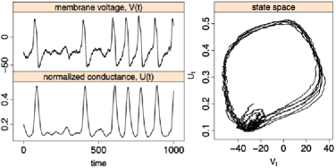
Figure 1: Simulated trajectory of the stochastic Morris–Lecar model: $(V_{t})$ as a function of time (left, top), $(U_{t})$ as a function of time (left, bottom), and $(U_{t})$ against $(V_{t})$ (right). Parameters are given in Section 6. Time is measured in ms, voltage in mV, and the conductance is normalized between 0 and 1.

2.2 Observations and approximate model

Data are discrete measurements of $(V_{t})$, while $(U_{t})$ is not measured. We denote $t_{0}\leq t_{1}\leq\cdots\leq t_{n}$ the discrete observation times. We denote $V_{i}=V_{t_{i}}$ the observation at time $t_{i}$ and $V_{0:n}=(V_{t_{0}},\ldots,V_{t_{n}})$ the vector of all the observed data. Let $\theta\in\Theta\subseteq\mathbb{R}^{p}$ be the vector of parameters to be estimated. We consider estimation of all identifiable parameters of the observed coordinate and the rate parameter of the unobserved channel dynamics $\theta=(g_{\mathrm{Ca}},g_{\mathrm{K}},g_{\mathrm{L}},V_{\mathrm{Ca}},V_{\mathrm{K}},I,\gamma,\phi)$. Note that $C$ is a proportionality factor of the conductance parameters and thus unidentifiable, as well as the constant level in $f(\cdot)$ is given by $g_{\mathrm{L}}V_{\mathrm{L}}+I$ and, thus, $V_{\mathrm{L}}$ (or $I$) is unidentifiable. We conjecture that the information about $\sigma$ in the observed coordinate is close to zero and, thus, in practice, also $\sigma$ is unidentifiable from observations of $V_{0:n}$ only, at least for any finite sample size. This happens because $\sigma$ is mainly shaping the dynamics of $U_{t}$ between spikes, while the dynamics during spikes resemble deterministic behavior, and the influence of $U_{t}$ on $V_{t}$ is only strong during spikes. This is confirmed in Sections 5 and 6 where misspecification of $\sigma$ is shown not to deteriorate the estimation of $\theta$. Finally, we assume the scaling parameters $V_{1}$–$V_{4}$ known because otherwise the model does not belong to an exponential family, as required by assumption (M1) below. This could be solved by introducing an extra optimization step in the EM algorithm at the cost of precision and computer time. It is not pursued further in this work.

The aim is to estimate $\theta$ by maximum likelihood. However, this likelihood is intractable, as the transition density of model (1) is not explicit. Let $\Delta$ denote the step size between two observation times, which for simplicity we assume do not depend on $i$. The extension to unequally spaced observation times is straightforward. The Euler–Maruyama approximation of model (1) leads to a discretized model defined as follows:

$$V_{i+1} = V_{i}+\Delta f(V_{i},U_{i})+\sqrt{\Delta}\gamma\tilde{\eta}_{i},$$

$$U_{i+1} = U_{i}+\Delta b(V_{i},U_{i})+\sqrt{\Delta}\sigma(V_{i},U_{i})\eta_{i},$$

where $(\tilde{\eta}_{i})$ and $(\eta_{i})$ are independent centered Gaussian variables. To ease readability, the same notation $(V_{i},U_{i})$ is used for the original and the approximated processes. This should not lead to confusion, as long as the transition densities are distinguished, as done below.

2.3 Property of the observation model

The observation model is a degenerate HMM. Let us recall the definition proposed by Cappé, Moulines and Rydén (2005). A HMM with not countable state space is defined as a bivariate Markov chain $(X_{i},Y_{i})$ with only partial observations $Y_{i}$, whose transition kernel has a special structure: both the joint process $(X_{i},Y_{i})$ and the marginal hidden chain $(X_{i})$ are Markovian.

In our model, $(U_{i})$ is not Markovian, only $(V_{i},U_{i})$ is Markovian. So set $X_{i}=(V_{i},U_{i})$, with Markov kernel $R(X_{i-1},dX_{i})=p_{\Delta}(dV_{i},dU_{i}|V_{i-1},U_{i-1})$, the transition density of model (2.2), and $Y_{i}=X_{i}^{(1)}$, the first coordinate of $X_{i}$ with transition kernel $F(X,dY)=\mathbh{1}_{\{Y=X^{(1)}\}}$. Here, $\mathbh{1}_{x}$ is the Dirac measure in $x$. Thus, the kernel $F$ is zero almost everywhere and the HMM is degenerate. This leads to an intrinsic degeneracy of the particle filter used in the standard HMM toolbox, as explained below.

Therefore, we consider the observation model as a bivariate Markov chain $(V_{i},U_{i})$ with only partial observations $V_{i}$ whose hidden coordinate $U_{i}$ is not Markovian. It is not a HMM but a general dynamic model as considered by Andrieu, Doucet and Punskaya (2001). The hidden process ${U_{i}}$ is distributed as

$$U_{0}\sim\mu(dU_{0}),\qquad U_{i}|(U_{0:i-1},V_{0:i-1})\sim K(dU_{i}|U_{0:i-1},V_{0:i-1})$$

for some conditional distribution function $K$ and the observed process $V_{i}$ is distributed as

$$V_{i}|(U_{0:i},V_{0:i-1})\sim G(dV_{i}|U_{0:i},V_{0:i-1})$$

for some distribution function $G$. Given the Markovian structure of the pair $(V_{i},U_{i})$, we have $K(dU_{i}|U_{0:i-1},V_{0:i-1})=K(dU_{i}|U_{i-1},V_{i-1})$ and $G(dV_{i}|U_{0:i},\allowbreak V_{0:i-1})=G(dV_{i}|U_{i-1:i},V_{i-1})$. To simplify, we use the same notation for random variables and their realizations and assume that $G(dV_{i}|U_{0:i}$, $V_{0:i-1})=G(V_{i}|U_{0:i},V_{0:i-1})\,dV_{i}$.

2.4 Likelihood function

We want to estimate the parameter $\theta$ by maximum likelihood of the approximate model, with likelihood

$$p_{\Delta}(V_{0:n};\theta)=\int p(V_{0},U_{0};\theta)\prod_{i=1}^{n}p_{\Delta}(V_{i},U_{i}|V_{i-1},U_{i-1};\theta)\,dU_{0:n}.$$ (3)

It corresponds to a pseudo-likelihood for the exact diffusion. The multiple integrals of equation (3) are difficult to handle and it is not possible to maximize the pseudo-likelihood directly.

A solution is to consider the statistical model as an incomplete data model. The observable vector $V_{0:n}$ is then part of a so-called complete vector $(V_{0:n},U_{0:n})$, where $U_{0:n}$ has to be imputed. To maximize the likelihood of the complete data vector $(V_{0:n},U_{0:n})$, we propose to use a stochastic version of the EM algorithm, namely, the SAEM algorithm [Delyon, Lavielle and Moulines (1999)]. Simulation under the smoothing distribution $p_{\Delta}(U_{0:n}|V_{0:n};\theta)$ is likely to be difficult, and direct simulation of the nonobserved data $(U_{0:n})$ is not possible. A SMC algorithm, also known as Particle Filtering, provides a way to approximate this distribution [Doucet, de Freitas and Gordon (2001)]. We have adapted this algorithm to handle a coupled two-dimensional SDE, that is, the unobserved coordinate is nonautonomous and non-Markovian. Then, we combine the SAEM algorithm with the SMC algorithm, where the unobserved data are filtered at each iteration step, to estimate the parameters of model (2.2). Details on the filtering are given in Section 3, and the SAEM algorithm is presented in Section 4.1. To prove the convergence of this new SAEM–SMC algorithm, a nonasymptotic deviation inequality is required for the SMC algorithm. Then we derive the convergence of the SAEM–SMC algorithm to a maximum of the likelihood.

3 Filtering

3.1 The filtering problem and the SMC algorithm

For any bounded Borel function $f\dvtx\mathbb{R}\mapsto\mathbb{R}$, we denote $\pi_{n,\theta}f=\mathbb{E}_{\Delta}(f(U_{n})|V_{0:n};\theta)$, the conditional expectation under the exact smoothing distribution $p_{\Delta}(U_{0:n}|V_{0:n};\theta)$ of the approximate model. The aim is to approximate this distribution for a fixed value of $\theta$. When included in the stochastic EM algorithm, this value will be the current value $\widehat{\theta}_{m}$ at the given iteration. For notational simplicity, $\theta$ is omitted in the rest of this section.

We now argue why the HMM point of view is ill-posed for the filtering problem. Considering the model as a HMM, $X_{i}=(V_{i},U_{i})$ is the hidden Markov chain and $Y_{i}=X_{i}^{(1)}$. But then the filtering problem $\pi_{n}f$ is the ratio of $\int\mu(dU_{0})R(X_{0},dX_{1})F(X_{0};Y_{1})\cdots R(X_{n-1},dX_{n})F(X_{n-1};Y_{n})f(X_{n})$ and$\int\mu(dU_{0})R(X_{0},dX_{1})F(X_{0};Y_{1})\cdots R(X_{n-1},dX_{n})F(X_{n-1};Y_{n})$. Since $F(X_{n-1};\allowbreak Y_{n})=\mathbh{1}_{\{Y_{n}=X_{n-1}^{(1)}\}}$ and the state space is continuous, the denominator is zero almost surely and the filtering problem is ill-posed.

Now consider the model in a more general framework with the hidden state $U_{i}$ not Markovian, and introduce for $i=1,\ldots,n$ the kernels $H_{i}$ from $\mathbb{R}$ into itself by

$$H_{i}f(u) = \int K(dz|u,V_{i-1})G(V_{i}|u,V_{i-1},z)f(z)$$

$$= \int p_{\Delta}(V_{i},z|V_{i-1},u)f(z)\,dz.$$

Then $\pi_{n}$ can be expressed recursively by

$$\pi_{n}f = \frac{\pi_{n-1}H_{n}f}{\pi_{n-1}H_{n}1}=\frac{\int\mu(U_{0})\prod_{i=1}^{n}p_{\Delta}(V_{i},U_{i}|V_{i-1},U_{i-1})f(U_{n})\,dU_{0:n}}{\int\mu(U_{0})\prod_{i=1}^{n}p_{\Delta}(V_{i},U_{i}|V_{i-1},U_{i-1})\,dU_{0:n}}.$$ (5)

Note that the denominator of (5) is $\mu H_{1}\cdots H_{n}1=p_{\Delta}(V_{0:n})$, which is different from 0 since its support is the real line. Thus, the filtering problem is well-posed.

The kernels $H_{i}$ are extensions of the kernels considered by Del Moral, Jacod and Protter (2001) in the context of two-dimensional SDEs with hidden coordinate $U_{t}$ autonomous (and thus Markovian). We do not extend their particle filter since it is based on simulation of both $V_{i}$ and $U_{i}$ with transition kernel $p_{\Delta}(V_{i},U_{i}|V_{i-1},U_{i-1})$. They avoid the degeneracy of the weights by introducing an instrumental function $\psi$ and the weights are computed as $\psi(V_{i}^{(k)}-V_{i})$. The choice of this instrumental function may influence the numerical properties of the filter. Therefore, we adopt the general filter proposed by Andrieu, Doucet and Punskaya (2001) for a more general dynamic system, that we recall here.

The SMC algorithm provides a set of $K$ particles $(U^{(k)}_{0:n})_{k=1,\dots,K}$ and weights $(W^{(k)}_{0:n})_{k=1,\dots,K}$ approximating the conditional smoothing distribution $p_{\Delta}(U_{0:n}|\allowbreak V_{0:n})$ [see Doucet, de Freitas and Gordon (2001)]. The SMC method relies on proposal distributions $q(U_{i}|V_{i},V_{i-1},U_{i-1})$ to sample what we call particles from these distributions. We write $V_{0:i}=(V_{0},\ldots,V_{i})$ and likewise for $U_{0:i}$.

Algorithm 1 ((SMC algorithm)).

• At time $i=0$: $\forall k=1,\ldots,K$:

  1. sample $U_{0}^{(k)}$ from $p(U_{0}|V_{0})$,

  2. compute and normalize the weights:

     $$w_{0}\bigl{(}U^{(k)}_{0}\bigr{)}=p\bigl{(}V_{0},U^{(k)}_{0}\bigr{)},\qquad W_{0}\bigl{(}U^{(k)}_{0}\bigr{)}=\frac{w_{0}(U^{(k)}_{0})}{\sum_{k=1}^{K}w_{0}(U^{(k)}_{0})}.$$

• At time $i=1,\ldots,n$: $\forall k=1,\ldots,K$:

  1. sample indices $A_{i-1}^{(k)}\sim r(\cdot|W_{i-1}(U_{0:i-1}^{(1)}),\ldots,W_{i-1}(U_{0:i-1}^{(K)}))$. Set $U_{0:i-1}^{\prime(k)}=U_{0:i-1}^{(A_{i-1}^{(k)})}$,

  2. sample $U^{(k)}_{i}\sim q(\cdot|V_{i-1:i},U^{\prime(k)}_{i-1})$ and set $U^{(k)}_{0:i}=(U_{0:i-1}^{\prime(k)},U^{(k)}_{i})$,

  3. compute and normalize the weights

     $$W_{i}\bigl{(}U^{(k)}_{0:i}\bigr{)} = \frac{w_{i}(U^{(k)}_{0:i})}{\sum_{k=1}^{K}w_{i}(U^{(k)}_{0:i})}\qquad\mbox{with }$$

     $$w_{i}\bigl{(}U^{(k)}_{0:i}\bigr{)} = \frac{p_{\Delta}(V_{0:i},U^{(k)}_{0:i})}{p_{\Delta}(V_{0:i-1},U_{0:i-1}^{\prime(k)})q(U^{(k)}_{i}|V_{i-1:i},U_{0:i-1}^{\prime(k)}).}$$

The SMC algorithm provides an empirical measure $\Psi^{K}_{n}=\break\sum_{k=1}^{K}W_{n}(U_{0:n}^{(k)})\mathbh{1}_{U_{0:n}^{(k)}}$ which is an approximation to the smoothing distribution $p_{\Delta}(U_{0:n}|V_{0:n})$. A draw from this distribution can be obtained by sampling an index $k$ from a multinomial distribution with probabilities $W_{n}(U_{0:n}^{(1)}),\ldots,W_{n}(U_{0:n}^{(K)})$ and setting the draw $U_{0:n}$ equal to $U_{0:n}=U^{(k)}_{0:n}$.

The variable $A_{i-1}^{(k)}$ plays an important role to discard the samples with small weights and multiply those with large weights [Gordon, Salmond and Smith (1993)]. It generates a number of offspring $N_{i-1}^{(\ell)}$, $\ell=1,\ldots,K$, such that $\sum_{\ell=1}^{K}N_{i-1}^{(\ell)}=K$ and $\mathbb{E}(N_{i-1}^{(\ell)})=KW_{i-1}(U^{(l)}_{0:i-1})$. Many schemes for $r$ have been presented in the literature, including multinomial sampling [Gordon, Salmond and Smith (1993)], residual sampling [Liu and Chen (1998)] or stratified resampling [Doucet, Godsill and Andrieu (2000)]. They differ in terms of $\operatorname{var}(N_{i-1}^{(\ell)})$ [see Doucet, Godsill and Andrieu (2000)]. The key property that we need in order to prove the deviation inequality is that $\mathbb{E}(\mathbh{1}_{\{A_{i-1}^{(k)}=\ell\}})=W_{i-1}(U^{(l)}_{0:i-1})$.

Since our model is not a HMM, the weights $w_{i}(U^{(k)}_{0:i})$ cannot be written in terms of a Markov transition kernel of the hidden path as is usually done. It follows that the proposal $q$, which is crucial to ensure good convergence properties, has to depend on $V_{i}$. The first classical choice of $q$ is $q(U_{i}|V_{i-1:i},U_{i-1})=p_{\Delta}(U_{i}|V_{i-1},U_{i-1})$, that is, the transition density. In this case, the weight reduces to $w_{i}(U^{(k)}_{0:i})=p_{\Delta}(V_{i}|V_{i-1},U^{(k)}_{0:i})$. A second choice for the proposal is $q(U_{i}|V_{i-1:i},U_{i-1})=p_{\Delta}(U_{i}|V_{i-1:i},U_{i-1})$, that is, the conditional distribution. In this case, the weight reduces to $w_{i}(U^{(k)}_{0:i})=p_{\Delta}(V_{i}|V_{i-1},U^{(k)}_{0:i-1})$. Transition densities and conditional distributions are detailed in Appendix A. When the two Brownian motions are independent, as we assume, the two choices are equivalent.

This SMC algorithm is plugged into the EM algorithm to estimate the parameters. We thus need nonasymptotic convergence results on the SMC algorithm to ensure the convergence of the EM algorithm. This is discussed in the next section.

3.2 Deviation inequality

In the literature, deviation inequalities forSMC algorithms only appear for HMM. To our knowledge, this is the first nonasymptotic result proposed for a SMC applied to a non-Markovian hidden path. The only result of this type with SDEs has been obtained by Del Moral, Jacod and Protter (2001), with autonomous second coordinate. Here, we generalize their deviation inequality to a nonautonomous hidden path.

For a bounded Borel function $f$, denote $\Psi_{n}^{K}f=\sum_{k=1}^{K}f(U_{n}^{(k)})W_{n,\theta}(U_{0:n}^{(k)})$, the conditional expectation of $f$ under the empirical measure $\Psi_{n,\theta}^{K}$ obtained by the SMC algorithm for a given value of $\theta$. We have the following:

Proposition 1

Under assumption (SMC3), for any $\varepsilon>0$, and for any bounded Borel function $f$ on $\mathbb{R}$, there exist constants $C_{1}$ and $C_{2}$, independent of $\theta$, such that

$$\mathbb{P}\bigl{(}\bigl{|}\Psi_{n,\theta}^{K}f-\pi_{n,\theta}f\bigr{|}\geq\varepsilon\bigr{)} \leq C_{1}\exp\biggl{(}-K\frac{\varepsilon^{2}}{C_{2}\|f\|^{2}}\biggr{)},$$ (6)

where $\|f\|$ is the sup-norm of $f$.

The proof is provided in Appendix D. A similar result can be obtained with respect to the exact smoothing distribution of the exact diffusion model, under assumptions on the number of particles and the step size of the Euler approximation.

4 Estimation method

4.1 SAEM algorithm

The EM algorithm [Dempster, Laird and Rubin (1977)] is useful in situations where the direct maximization of the marginal likelihood $\theta\rightarrow p_{\Delta}(V_{0:n};\theta)$ is more difficult than the maximization of the conditional expectation of the complete likelihood $Q(\theta|\theta^{\prime})=\mathbb{E}_{\Delta}[\log p_{\Delta}(V_{0:n},U_{0:n};\theta)|V_{0:n};\theta^{\prime}]$, where $p_{\Delta}(V_{0:n},U_{0:n};\theta)$ is the likelihood of the complete data $(V_{0:n},U_{0:n})$ of the approximate model (2.2) and the expectation is under the conditional distribution of $U_{0:n}$ given $V_{0:n}$ with density $p_{\Delta}(U_{0:n}|V_{0:n};\theta^{\prime})$. The EM algorithm is an iterative procedure: at the $m$th iteration, given the current value $\widehat{\theta}_{m-1}$, the E-step is the evaluation of $Q_{m}(\theta)=Q(\theta|\widehat{\theta}_{m-1})$, while the M-step updates $\widehat{\theta}_{m-1}$ by maximizing $Q_{m}(\theta)$. To fulfill convergence conditions of the algorithm, we consider the particular case of a distribution from an exponential family. More precisely, we assume the following:

• [(M1)]

• The parameter space $\Theta$ is an open subset of $\mathbb{R}^{p}$. The complete likelihood $p_{\Delta}(V_{0:n},U_{0:n};\theta)$ belongs to a curved exponential family, that is, $\log p_{\Delta}(V_{0:n},U_{0:n};\theta)=-\psi(\theta)+\langle S(V_{0:n},U_{0:n}),\nu(\theta)\rangle$, where $\psi$ and $\nu$ are two functions of $\theta$, $S(V_{0:n},U_{0:n})$ is known as the minimal sufficient statistic of the complete model, taking its value in a subset ${\mathcal{S}}$ of $\mathbb{R}^{d}$, and $\langle\cdot,\cdot\rangle$ is the scalar product on $\mathbb{R}^{d}$.

The approximate Morris–Lecar model (2.2) satisfies this assumption when the scaling parameters $V_{1},V_{2},V_{3}$ and $V_{4}$ are known. Details of the sufficient statistic $S$ are given in Appendix B.

Under assumption (M1), the E-step reduces to the computation of$\mathbb{E}_{\Delta}[S(V_{0:n},\allowbreak U_{0:n})|V_{0:n};\widehat{\theta}_{m-1}]$. When this expectation has no closed form, Delyon, Lavielle and Moulines (1999) propose the Stochastic Approximation EM algorithm (SAEM), replacing the E-step by a stochastic approximation of $Q_{m}(\theta)$. The E-step is then divided into a simulation step (S-step) of the nonobserved data $(U_{0:n}^{(m)})$ with the conditional density $p_{\Delta}(U_{0:n}|V_{0:n};\widehat{\theta}_{m-1})$ and a stochastic approximation step (SA-step) of $\mathbb{E}_{\Delta}[S(V_{0:n},U_{0:n})|V_{0:n};\widehat{\theta}_{m-1}]$ with a sequence of positive numbers $(a_{m})_{m\in\mathbb{N}}$ decreasing to zero. We write $s_{m}$ for the approximation of this expectation. At the S-step, the simulation under the smoothing distribution is done by SMC, as explained in Section 3. We call this algorithm the SAEM–SMC algorithm. Iterations of the SAEM–SMC algorithm are written as follows:

Algorithm 2 ((SAEM–SMC algorithm)).

• Iteration $0$: initialization of $\widehat{\theta}_{0}$ and set $s_{0}=0$.

• Iteration $m\geq 1$:

  • [SA-step:]

  • simulation of the nonobserved data $(U_{0:n}^{(m)})$ with SMC targeting the distribution $p_{\Delta}(U_{0:n}|V_{0:n};\widehat{\theta}_{m-1})$.

  • update $s_{m-1}$ using the stochastic approximation:

    $$s_{m}=s_{m-1}+a_{m-1}\bigl{[}S\bigl{(}V_{0:n},U_{0:n}^{(m)}\bigr{)}-s_{m-1}\bigr{]}.$$ (7)

  • update of $\widehat{\theta}_{m}$ by $\widehat{\theta}_{m}=\operatorname{\arg\max}_{\theta\in\Theta}(-\psi(\theta)+\langle s_{m},\nu(\theta)\rangle)$.

Standard errors of the estimators can be evaluated through the Fisher information matrix. Details are given in Appendix C. An advantage of the SAEM algorithm is the low-level dependence on the initialization $\widehat{\theta}_{0}$, due to the stochastic approximation of the E-step. The other advantage over a Monte Carlo EM algorithm is the computational time. Indeed, only one simulation of the hidden variables $U_{0:n}$ is needed in the simulation step, while an increasing number of simulated hidden variables is required in a Monte Carlo EM algorithm.

4.2 Convergence of the SAEM–SMC algorithm

The SAEM algorithm we propose in this paper is based on an approximate simulation step performed with an SMC algorithm. We prove that even if this simulation is not exact, the SAEM algorithm still converges toward the maximum of the likelihood of the approximated diffusion (2.2). This is true because the SMC algorithm has good convergence properties.

Let us be more precise. We introduce a set of convergence assumptions which are the classic ones for the SAEM algorithm [Delyon, Lavielle and Moulines (1999)]:

• [(SAEM3)]

• The functions $\psi(\theta)$ and $\nu(\theta)$ are twice continuously differentiable on $\Theta$.

• The function $\bar{s}\dvtx\Theta\longrightarrow\mathcal{S}$ defined by $\bar{s}(\theta)=\int S(v,u)p_{\Delta}(u|v;\theta)\,dv\,du$ is continuously differentiable on $\Theta$.

• The function $\ell_{\Delta}(\theta)=\log p_{\Delta}(v,u,\theta)$ is continuously differentiable on $\Theta$ and $\partial_{\theta}\int p_{\Delta}(v,u;\theta)\,dv\,du=\int\partial_{\theta}p_{\Delta}(v,u;\theta)\,dv\,du$.

• Define $L\dvtx\mathcal{S}\times\Theta\rightarrow\mathbb{R}$ by $L(s,\theta)=-\psi(\theta)+\langle s,\nu(\theta)\rangle$. There exists a function $\hat{\theta}\dvtx\mathcal{S}\rightarrow\Theta$ such that $\forall\theta\in\Theta,\forall s\in\mathcal{S},L(s,\hat{\theta}(s))\geq L(s,\theta)$.

• The positive decreasing sequence of the stochastic approximation $(a_{m})_{m\geq 1}$ is such that $\sum_{m}a_{m}=\infty$ and $\sum_{m}a^{2}_{m}<\infty$.

• $\ell_{\Delta}\dvtx\Theta\rightarrow\mathbb{R}$ and $\hat{\theta}\dvtx\mathcal{S}\rightarrow\Theta$ are $d$ times differentiable, where $d$ is the dimension of $S(v,u)$.

• For all $\theta\in\Theta$, $\int\|S(v,u)\|^{2}p_{\Delta}(u|v;\theta)\,du<\infty$ and the function $\Gamma(\theta)=\operatorname{Cov}_{\theta}(S(\cdot,U_{0:n}))$ is continuous, where the covariance is under the conditional distribution $p_{\Delta}(U_{0:n}|V_{0:n};\theta)$.

• Let $\{\mathcal{F}_{m}\}$ be the increasing family of $\sigma$-algebras generated by the random variables $s_{0},U_{0:n}^{(1)}$, $U_{0:n}^{(2)},\ldots,U_{0:n}^{(m)}$. For any positive Borel function $f$, $\mathbb{E}_{\Delta}(f(U_{0:n}^{(m+1)})|\mathcal{F}_{m})=\int f(u)p_{\Delta}(u|v,\widehat{\theta}_{m})\,du$.

Assumptions (M1)–(M5) ensure the convergence of the EM algorithm when the E-step is exact [Delyon, Lavielle and Moulines (1999)]. Assumptions (M1)–(M5) and (SAEM1)–(SAEM4) together with the additional assumption that $(s_{m})_{m\geq 0}$ takes its values in a compact subset of $\mathcal{S}$ ensure the convergence of the SAEM estimates to a stationary point of the observed likelihood $p_{\Delta}(V_{0:n};\theta)$ when the simulation step is exact [Delyon, Lavielle and Moulines (1999)].

Here the simulation step is not exact and we have three additional assumptions on the SMC algorithm to bound the error induced by this algorithm and prove the convergence of the SAEM–SMC algorithm:

• [(SMC3)]

• The number of particles $K$ used at each iteration of the SAEM algorithm varies along the iteration: there exists a function $g(m)\rightarrow\infty$ when $m\rightarrow\infty$ such that $K(m)\geq g(m)\log(m)$.

• The function $S$ is bounded uniformly in $u$.

• The functions $p_{\Delta}(V_{i}|U_{i},V_{i-1},U_{i-1};\theta)$ are bounded uniformly in $\theta$.

Theorem 1

Assume that (M1)–(M5), (SAEM1)–(SAEM3) and (SMC1)–(SMC3) hold. Then, with probability 1, $\lim_{m\rightarrow\infty}$ $d(\widehat{\theta}_{m},\mathcal{L})=0$, where $\mathcal{L}=\{\theta\in\Theta,\partial_{\theta}\ell_{\Delta}(\theta)=0\}$ is the set of stationary points of the log-likelihood$\ell_{\Delta}(\theta)=\log p_{\Delta}(V_{0:n};\theta)$.

Theorem 1 is proved in Appendix D. Note that assumption (SAEM4) is not needed thanks to the conditional independence of the particles generated by the SMC algorithm, as detailed in the proof. Similarly, the additional assumption that $(s_{m})_{m\geq 0}$ takes its values in a compact subset of $\mathcal{S}$ is not needed, as it is directly satisfied under assumption (SMC2).

We deduce that the SAEM algorithm converges to a (local) maximum of the likelihood under standard additional assumptions (LOC1)–(LOC3) proposed by Delyon, Lavielle and Moulines (1999) on the regularity of the log-likelihood $\ell_{\Delta}(V_{0:n};\theta)$ that we do not recall here.

Corollary 1

Under the assumptions of Theorem 1 and additional assumptions (LOC1)–(LOC3), the sequence $\widehat{\theta}_{m}$ converges with probability 1 to a (local) maximum of the likelihood $p_{\Delta}(V_{0:n};\theta)$.

The classical assumptions (M1)–(M5) are usually satisfied. Assumption (SAEM1) is easily satisfied by choosing properly the sequence $(a_{m})$. Assumptions (SAEM2) and (SAEM3) depend on the regularity of the model. They are satisfied for the approximate Morris–Lecar model.

In practice, the SAEM algorithm is implemented with an increasing number equal to the iteration number, which satisfies Assumption (SMC1). Assumption (SMC2) is satisfied for the approximate Morris–Lecar model because the variables $U$ are bounded between 0 and 1 and the variables $V$ are fixed at their observed values. This would not have been the case with the filter of Del Moral, Jacod and Protter (2001), which resimulates the variables $V$ at each iteration. Assumption (SMC3) is satisfied if we require that $\gamma$ is strictly bounded away from zero; $\gamma\geq\varepsilon>0$.

4.3 Properties of the approximate diffusion

The SAEM–SMC algorithm provides a sequence which converges to the set of stationary points of the log-likelihood $\ell_{\Delta}(\theta)=\log p_{\Delta}(V_{0:n};\theta)$. The following result aims at comparing this likelihood, which corresponds to the Euler approximate model (2.2), with the true likelihood $p(V_{0:n};\theta)$. The result is based on the bound of the Euler approximation proved by Gobet and Labart (2008). Their result holds under the following assumption:

• [(H1)]

• Functions $f$, $b$, $\sigma$ are 2 times differentiable with bounded derivatives with respect to $u$ and $v$ of all orders up to 2.

Let us assume we apply the SAEM algorithm on an approximate model obtained with an Euler scheme of step size $\delta=\Delta/L$. Then we have the following:

Theorem 2

Under assumption (H1), there exists a constant $C$, independent of $\theta$, such that for any $\theta\in\Theta$ and any vector $V_{0:n}$,

$$\bigl{|}p(V_{0:n};\theta)-p_{\delta}(V_{0:n};\theta)\bigr{|}\leq C\frac{1}{L}n\Delta.$$

Proof is given in Appendix D. Assumption (H1) is a strong assumption, which is sufficient and not necessary. It does not hold for the Morris–Lecar model. Different sets of weaker assumptions have been proposed to prove the convergence of the Euler scheme in the strong sense (expectation of the absolute error between the exact and approximated process). The proofs are mainly based on localization arguments; see Kloeden and Neuenkirch (2012) for a review paper. The convergence of the densities has been less studied, and it is beyond the scope of this paper.

5 Intracellular recordings from a turtle motoneuron

The membrane potential from a spinal motoneuron in segment D10 of an adult red-eared turtle (Trachemys scripta elegans) was recorded while a periodic mechanical stimulus was applied to selected regions of the carapace with a sampling step of 0.1 ms [for details see Berg, Alaburda and Hounsgaard (2007), Berg, Ditlevsen and Hounsgaard (2008)]. The turtle responds to the stimulus with a reflex movement of a limb known as the scratch reflex, causing an intense synaptic input to the recorded neuron. Due to the time-varying stimulus, a model for the complete data set needs to incorporate the time inhomogeneity, as done in Jahn et al. (2011). However, in Jahn et al. (2011), only one-dimensional diffusions are considered, and spikes are modeled as single points in time by adding a jump term with state-dependent intensity function to the SDE, ignoring the detailed dynamics during spikes. In this paper we aim at estimating parameters during spiking activity by explicit modeling of time-varying conductances. Therefore, we only analyze four traces during on-cycles [following Jahn et al. (2011)] where spikes occur. Furthermore, in these time windows, the input is approximately constant, which is required for the Morris–Lecar model with constant parameters. An example of the analyzed data is plotted in Figure 2, together with a filtered trace of the unobserved coordinate.

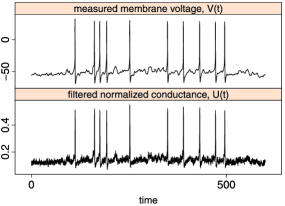
Figure 2: Observations of the membrane potential in a spinal motoneuron of an adult red-eared turtle during 600 ms (upper panel) and the filtered hidden process of the normalized conductance associated with K⁺ current (lower panel) for the estimated parameters with the scaling parameters fixed at $V_{1}=-2.4$ mV, $V_{2}=36$ mV, $V_{3}=4$ mV and $V_{4}=60$ mV.

Table 1: Parameter estimates obtained from observations of the membrane potential of a spinal motoneuron of an adult red-eared turtle during 600 ms for two different sets of scaling parameters. With $\sigma=0.05$ fixed. First trace

	Parameter
	$\bm{g_{\mathrm{L}}}$	$\bm{g_{\mathrm{Ca}}}$	$\bm{g_{\mathrm{K}}}$	$\bm{\gamma}$	$\bm{V_{\mathrm{K}}}$	$\bm{\phi}$	$\bm{V_{\mathrm{Ca}}}$	$\bm{I}$
With $V_{1}=-1.2$ mV, $V_{2}=18$ mV, $V_{3}=2$ mV, $V_{4}=30$ mV
Estimate	$-0.296$	$11.274$	$6.553$	$2.801$	$-124.481$	$1.989$	$35.769$	$-5.024$
SE	$0.001$	$0.028$	$0.049$	$0.001$	$14.563$	$0.000$	$0.122$	$0.052$
With $V_{1}=-2.4$ mV, $V_{2}=36$ mV, $V_{3}=4$ mV, $V_{4}=60$ mV
Estimate	$1.046$	$12.906$	$20.878$	$2.466$	$-67.097$	$2.153$	$98.698$	$-65.403$
SE	$0.009$	$0.008$	$0.021$	$0.001$	$0.227$	$0.001$	$0.198$	$1.204$

First the model was fitted with the values of the scaling parameters $V_{1}$–$V_{4}$ given in Rinzel and Ermentrout (1989) and used in Section 6 below; see Table 1 for one of the traces. Most of the estimates are reasonable and in agreement with the expected order of magnitudes for the parameter values, except for the $V_{\mathrm{Ca}}$ reversal potential, which in the literature is reported to be around 100–150 mV (estimated to 44.7 mV), and the leak conductance, which is estimated to be negative. Conductances are always nonnegative. This is probably due to wrong choices of the scaling constants $V_{1}$–$V_{4}$. For the parameters given in Rinzel and Ermentrout (1989), the average of the membrane potential $V_{t}$ between spikes is around $-$26 mV, whereas the average of the experimental trace between spikes is around $-$56 mV, a factor two larger. We therefore rerun the estimation procedure fixing $V_{1}$–$V_{4}$ to twice the value from before, which provides approximately the same values of the normalized Ca²⁺ conductance, $m_{\infty}(\cdot)$, and the rates of opening and closing of K⁺ ion channels, $\alpha(\cdot)$ and $\beta(\cdot)$, as in the theoretical model when $V_{t}$ is at its equilibrium value. In this case all parameters are reasonable and in agreement with the expected order of magnitudes.

Table 2: Parameter estimates obtained from observations of the membrane potential of a spinal motoneuron of an adult red-eared turtle during 600 ms for three different values of $\sigma$. With $V_{1}=-2.4$ mV, $V_{2}=36$ mV, $V_{3}=4$ mV, $V_{4}=60$ mV fixed. First trace

	Parameter
	$\bm{g_{\mathrm{L}}}$	$\bm{g_{\mathrm{Ca}}}$	$\bm{g_{\mathrm{K}}}$	$\bm{\gamma}$	$\bm{V_{\mathrm{K}}}$	$\bm{\phi}$	$\bm{V_{\mathrm{Ca}}}$	$\bm{I}$
$\sigma$ fixed to 0.02
Estimate	$1.302$	$12.460$	$16.550$	$2.280$	$-74.301$	$2.881$	$99.398$	$-52.742$
SE	$0.003$	$0.028$	$0.131$	$0.000$	$0.703$	$0.001$	$2.384$	$2.727$
$\sigma$ fixed to 0.05
Estimate	$1.046$	$12.906$	$20.878$	$2.466$	$-67.097$	$2.153$	$98.698$	$-65.403$
SE	$0.009$	$0.008$	$0.021$	$0.001$	$0.227$	$0.001$	$0.198$	$1.204$
$\sigma$ fixed to 0.15
Estimate	$1.308$	$12.442$	$16.419$	$2.301$	$-74.576$	$2.911$	$99.417$	$-52.341$
SE	$0.002$	$0.007$	$0.120$	$0.000$	$0.021$	$0.000$	$4.529$	$1.558$

Table 3: Parameter estimates obtained from four different traces of the membrane potential of a spinal motoneuron of an adult red-eared turtle. Each trace has 6000 observations points with a sampling step of 0.1 ms. With $V_{1}=-2.4$ mV, $V_{2}=36$ mV, $V_{3}=4$ mV, $V_{4}=60$ mV and $\sigma=0.05$ fixed

	Parameter
	$\bm{g_{\mathrm{L}}}$	$\bm{g_{\mathrm{Ca}}}$	$\bm{g_{\mathrm{K}}}$	$\bm{\gamma}$	$\bm{V_{\mathrm{K}}}$	$\bm{\phi}$	$\bm{V_{\mathrm{Ca}}}$	$\bm{I}$
First trace
Estimate	$1.046$	$12.906$	$20.878$	$2.466$	$-67.097$	$2.153$	$98.698$	$-65.403$
SE	$0.009$	$0.008$	$0.021$	$0.001$	$0.227$	$0.001$	$0.198$	$1.204$
Second trace
Estimate	$1.430$	$11.705$	$15.791$	$2.253$	$-73.029$	$3.138$	$103.709$	$-53.183$
SE	$0.003$	$0.008$	$0.029$	$0.000$	$0.641$	$0.001$	$1.269$	$0.651$
Third trace
Estimate	$1.371$	$11.878$	$15.379$	$2.210$	$-75.024$	$3.004$	$99.887$	$-49.499$
SE	$0.002$	$0.013$	$0.017$	$0.000$	$0.195$	$0.000$	$0.464$	$0.614$
Fourth trace
Estimate	$1.197$	$11.452$	$12.521$	$2.012$	$-85.982$	$3.776$	$99.615$	$-37.017$
SE	$0.002$	$0.055$	$0.017$	$0.000$	$0.089$	$0.000$	$1.466$	$0.861$

To check the robustness to misspecifications in the diffusion parameter $\sigma$ of the unobserved coordinate, we fitted the model for three different values of $\sigma$; see Table 2. Results are stable and suggest that $\sigma$ is primarily affecting the subthreshold fluctuations of the channel dynamics, and mainly the spiking dynamics of the unobserved coordinate influences the first coordinate.

Final results for all four traces are presented in Table 3. It is reassuring that the parameter estimates seem so reproducible over different traces; the largest variation was below 10%. This is not due to starting values, for example, the starting value for $g_{\mathrm{L}}$ was 0.1, and all four estimates ended up between 1.3 and 1.4, and the starting value for $V_{\mathrm{K}}$ was $-55$, and all four estimates ended up between $-75.4$ and $-74.4$.

6 Simulation study

Parameter values of the Morris–Lecar model used in the simulations are the same as those of Rinzel and Ermentrout (1989), Tateno and Pakdaman (2004) for a class II membrane, except that we set the membrane capacitance constant to $C=1$ $\mu$F$/$cm², which is the standard value reported in the literature. Conductances and input current were correspondingly changed and, thus, the two models are the same. The values are as follows: $V_{\mathrm{K}}=-84$ mV, $V_{\mathrm{L}}=-60$ mV, $V_{\mathrm{Ca}}=120$ mV, $C=1$ $\mu$F$/$cm², $g_{\mathrm{L}}=0.1$ $\mu$S$/$cm², $g_{\mathrm{Ca}}=0.22$ $\mu$S$/$cm², $g_{\mathrm{K}}=0.4$ $\mu$S$/$cm², $V_{1}=-1.2$ mV, $V_{2}=18$ mV, $V_{3}=2$ mV, $V_{4}=30$ mV, $\phi=0.04$ ms^-1. Input is chosen to be $I=4.5$ $\mu$A$/$cm². Initial conditions of the Morris–Lecar model are $V_{t_{0}}=-26$ mV, $U_{t_{0}}=0.2$. The volatility parameters are $\gamma=1$ mV ms^-1/2, $\sigma=0.03$ $\mbox{ms}^{-1/2}$. Trajectories are simulated with time step $\delta=0.01$ ms and $n=2000$ points are subsampled with observations time step $\Delta=10\delta$. Then $\theta$ is estimated on each simulated trajectory. A hundred repetitions are used to evaluate the performance of the estimators. An example of a simulated trajectory (for $n=10\mbox{,}000$) is given in Figure 1.

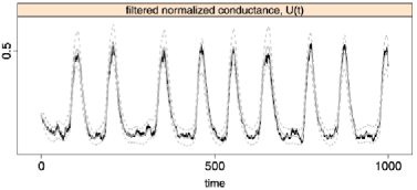
Figure 3: Filtering of $(U_{t})$ with the particle filter algorithm (100 particles): hidden simulated trajectory of the Morris–Lecar model $(U_{t})$ (black), mean filtered signal (grey full drawn line), 95% confidence interval of filtered signal (grey dashed lines).

6.1 Filtering results

The Particle filter aims at filtering the hidden process $(U_{t})$ from the observed process $(V_{t})$. We illustrate its performance on a simulated trajectory, with $\theta$ fixed at its true value. The SMC Particle filter algorithm is implemented with $K=100$ particles and the transition density as proposal; see Figure 3. The true hidden process, the mean filtered signal and its 95% confidence interval are plotted. The filtered process appears satisfactory. The confidence interval includes the true hidden process $(U_{t})$.

6.2 Estimation results

The performance of the SAEM–SMC algorithm is illustrated on 100 simulated trajectories. The SAEM algorithm is implemented with $m=200$ iterations and a sequence ($a_{m}$) equal to 1 during the 100 first iterations and equal to $a_{m}=1/(m-100)^{0.8}$ for $m>100$. The SMC algorithm is implemented with $K(m)=\min(m,100)$ particles at each iteration of the SAEM algorithm. The SAEM algorithm is initialized by a random draw of $\widehat{\theta}_{0}$ not centered around the true value: $\widehat{\theta}_{0}=\theta_{\mathrm{true}}+0.1+\theta_{\mathrm{true}}/3\mathcal{N}(0,1)$.

An example of the convergence of the SAEM algorithm for one of the iterations is presented in Figure 4. It is seen that the algorithm converges for most of the parameters in a few iterations to a neighborhood of the true value, even if the initial values are far from the true ones. Only for $\phi$ more iterations are needed, which is expected since this parameter appears in the second, nonobserved coordinate.

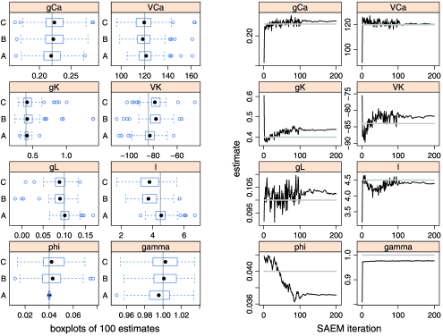
Figure 4: Estimation results for simulated data. Left panels: Boxplots of 100 estimates from simulated data sets for the 8 parameters. True values used in the simulations are given by the gray lines. A: Both $V_{t}$ and $U_{t}$ are observed. B: Only $V_{t}$ is observed, $\sigma$ is fixed at the true value 0.03. C: Only $V_{t}$ is observed, $\sigma$ is fixed at a wrong value 0.04. Right panels: Convergence of the SAEM algorithm for the 8 estimated parameters on a simulated data set. True values used in the simulation are given by the gray lines.

Table 4: Simulation results obtained from 100 simulated Morris–Lecar trajectories ($n=2000$, $\Delta=0.1$ ms). Two estimators are compared: The pseudo maximum likelihood estimator in the ideal case where both $V_{t}$ and $U_{t}$ are observed, and the SAEM estimator when only $V_{t}$ is observed with the SAEM initialization at a random value not centered around the true value $\theta$. An example of standard errors (SE) estimated with the SAEM–SMC algorithm on one single simulated data set is also given

	Parameter
Estimator	$\bm{g_{\mathrm{L}}}$	$\bm{g_{\mathrm{Ca}}}$	$\bm{g_{\mathrm{K}}}$	$\bm{\gamma}$	$\bm{V_{\mathrm{K}}}$	$\bm{\phi}$	$\bm{V_{\mathrm{Ca}}}$	$\bm{I}$
True values:	$\bm{0.100}$	$\bm{0.220}$	$\bm{0.400}$	$\bm{1.00}$	$\bm{-84.00}$	$\bm{0.040}$	$\bm{120.00}$	$\bm{4.400}$
With both $V_{t}$ and $U_{t}$ observed (pseudo maximum likelihood estimator)
Mean	$0.101$	$0.219$	$0.411$	$0.996$	$-83.20$	$0.040$	$121.97$	$4.539$
RMSE	$0.017$	$0.019$	$0.041$	$0.019$	$7.61$	$0.001$	$8.50$	$0.560$
With only $V_{t}$ observed (SAEM estimator)
Mean	$0.090$	$0.225$	$0.464$	$1.003$	$-78.622$	$0.041$	$119.677$	$4.060$
RMSE	$0.021$	$0.024$	$0.144$	$0.017$	$9.459$	$0.013$	$10.218$	$1.028$
Estimated SE	$0.016$	$0.019$	$0.042$	$0.016$	$4.96$	$0.001$	$7.31$	$0.561$

The SAEM estimator is compared with the pseudo maximum likelihood estimator obtained if both $V_{t}$ and $U_{t}$ were observed. Results are given in Table 4. The parameters are well estimated in this ideal case. The estimation of $\phi$, which is the only parameter in the drift of the hidden coordinate $U_{t}$, is good and does not deteriorate the estimation of the other parameters. In Figure 4 we show boxplots of the estimates of the eight parameters for the three estimation settings; both coordinates observed or only one observed with $\sigma$ fixed at either the true or a wrong value. All parameters appear well estimated. As expected, the variance of the estimator of $\phi$ hugely increases when only one coordinate is observed, but interestingly, the variance of the parameters of the observed coordinate do not seem much affected by this loss of information.

The SAEM–SMC algorithm provides estimates of the standard errors (SE) of the estimators (see Appendix C). These should be close to the RMSE obtained from the 100 simulated data sets. As an example, the SE for one data set estimated by SAEM are reported in the last line of Table 4. The estimated SE are satisfactory for most of the parameters, but tend to underestimate.

7 Discussion

The main contributions of this paper are an algorithm to handle a more general model than a HMM and to show nonasymptotic convergence results for the method. It turns out that some of the common problems encountered with particle filters are not present in our case, namely, the filter does not degenerate, and we run the algorithm on large data sets of 6000 observations points in reasonable time (35 minutes on a standard portable computer for one of the simulated data sets).

To the authors’ knowledge, this is the first time the rate parameter of the unobserved coordinate, $\phi$, is estimated from experimental data. It is comforting to observe that the estimated value does not seem to be very sensitive to the choice of scaling parameters. Other parameters, like the conductances and the reversal potentials, are more sensitive to this choice, and should be interpreted with care.

The estimation procedure builds on the pseudo likelihood, which approximates the true likelihood by an Euler scheme. This approximation is only valid for a small sampling step, that is, for high frequency data, which is the case for the type of neuronal data considered here. If data were sampled less often, a possibility could be to simulate diffusion bridges between the observed points and apply the estimation procedure to an augmented data set consisting of the observed data and the imputed values.

There are several issues that deserve further study. First, it is important to understand the influence of the scaling parameters $V_{1}$–$V_{4}$ and how to estimate them for a given data set. The model is not exponential in these parameters [assumption (M1)] and new estimation procedures have to be considered. Second, one should be aware of the possible misspecification of the model. More detailed models incorporating further types of ion channels could be explored, but increasing the model complexity might deteriorate the estimates, since the information contained in only observing the membrane potential is limited. Furthermore, the sensitivity on the choice of tuning parameters of the algorithm, like the decreasing sequence of the stochastic approximation, $(a_{m})$, and the number of SAEM iterations, needs further investigation. Finally, an automated procedure to find starting values for the procedure is warranted.

Appendix A Distributions of approximate model

Consider the general approximate model [see (2.2)]

$$\pmatrix{V_{i+1}\cr U_{i+1}}=\pmatrix{V_{i}\cr U_{i}}+\Delta\pmatrix{f(V_{i},U_{i})\cr b(V_{i},U_{i})}+\sqrt{\Delta}\pmatrix{\gamma&\rho\cr\rho&\sigma(V_{i},U_{i})}\pmatrix{\tilde{\eta}_{i}\cr\eta_{i}}$$

with $\rho$ the correlation coefficient between the two Brownian motions or perturbations. The distribution of $(V_{i+1},U_{i+1})$ conditionally on $(V_{i},U_{i})$ is

$$\pmatrix{V_{i+1}\cr U_{i+1}}\Big{|}\pmatrix{V_{i}\cr U_{i}}$$

$$\qquad\sim\mathcal{N}\left(\biggl{[}\matrix{V_{i}+\Delta f(V_{i},U_{i})\cr U_{i}+\Delta b(V_{i},U_{i})}\biggr{]},\Delta\left[\matrix{\bigl{(}\gamma^{2}+\rho^{2}\bigr{)}&\rho\bigl{(}\gamma+\sigma(V_{i},U_{i})\bigr{)}\vspace*{2pt}\cr\rho\bigl{(}\gamma+\sigma(V_{i},U_{i})\bigr{)}&\bigl{(}\sigma^{2}(V_{i},U_{i})+\rho^{2}\bigr{)}}\right]\right).$$

The marginal distributions of $V_{i+1}$ conditionally on $(V_{i},U_{i})$ and $U_{i+1}$ conditionally on $(V_{i},U_{i})$ are

$$V_{i+1}|V_{i},U_{i} \sim \mathcal{N}\bigl{(}V_{i}+\Delta f(V_{i},U_{i}),\Delta\bigl{(}\gamma^{2}+\rho^{2}\bigr{)}\bigr{)},$$

$$U_{i+1}|V_{i},U_{i} \sim \mathcal{N}\bigl{(}U_{i}+\Delta b(V_{i},U_{i}),\Delta\bigl{(}\sigma^{2}(V_{i},U_{i})+\rho^{2}\bigr{)}\bigr{)}.$$

The conditional distributions of $V_{i+1}$ conditionally on $(U_{i+1},V_{i},U_{i})$ and $U_{i+1}$ conditionally on $(V_{i+1},V_{i},U_{i})$ are

$$V_{i+1}|U_{i+1},V_{i},U_{i} \sim \mathcal{N}(m_{V},\mathit{Var}_{V}),$$

$$U_{i+1}|V_{i+1},V_{i},U_{i} \sim \mathcal{N}(m_{U},\mathit{Var}_{U}),$$

where

$$m_{V} = V_{i}+\Delta f(V_{i},U_{i})+\frac{\rho(\gamma+\sigma(V_{i},U_{i}))}{\sigma^{2}(V_{i},U_{i})+\rho^{2}}\bigl{(}U_{i+1}-U_{i}-\Delta b(V_{i},U_{i})\bigr{)},$$

$$\mathit{Var}_{V} = \Delta\bigl{(}\gamma^{2}+\rho^{2}\bigr{)}-\frac{\Delta\rho^{2}(\gamma+\sigma(V_{i},U_{i}))^{2}}{\sigma^{2}(V_{i},U_{i})+\rho^{2}},$$

$$m_{U} = U_{i}+\Delta b(V_{i},U_{i})+\frac{\rho(\gamma+\sigma(V_{i},U_{i}))}{\gamma^{2}+\rho^{2}}\bigl{(}V_{i+1}-V_{i}-\Delta f(V_{i},U_{i})\bigr{)},$$

$$\mathit{Var}_{U} = \Delta\bigl{(}\sigma^{2}(V_{i},U_{i})+\rho^{2}\bigr{)}-\frac{\Delta\rho^{2}(\gamma+\sigma(V_{i},U_{i}))^{2}}{\gamma^{2}+\rho^{2}}.$$

The distributions in (A) and (A) are equal when the Brownian motions are independent, that is, when $\rho=0$.

Appendix B Sufficient statistics

We here provide the sufficient statistics of the approximate model (2.2). Consider the $n\times 6$-matrix

$$X = \bigl{(}-V_{0:(n-1)},-m_{\infty}(V_{0:(n-1)})V_{0:(n-1)},$$

$$\hskip 5.0pt{}-U_{0:(n-1)}V_{0:(n-1)},U_{0:(n-1)},\bm{1},m_{\infty}(V_{0:(n-1)})\bigr{)},$$

where $\bm{1}$ is the vector of $1$’s of size $n$. Then the vector

$$S_{1}(V_{0:(n-1)},U_{0:(n-1)})=\bigl{(}X^{\prime}X\bigr{)}^{-1}X^{\prime}(V_{1:n}-V_{0:(n-1)})$$

is the sufficient statistic vector corresponding to the parameters $\nu_{1}(\theta)=(g_{\mathrm{L}},g_{\mathrm{Ca}},\allowbreak g_{\mathrm{K}},g_{\mathrm{K}}V_{\mathrm{K}},g_{\mathrm{L}}V_{\mathrm{L}}+I,g_{\mathrm{Ca}}V_{\mathrm{Ca}})$, where ^′ denotes transposition.

The sufficient statistics corresponding to $\nu_{2}(\theta)=1/\gamma^{2}$ are

$$\displaystyle\sum_{i=1}^{n}(V_{i}-V_{i-1})U_{i-1},\qquad\sum_{i=1}^{n}U_{i-1}^{2},\qquad\sum_{i=1}^{n}(V_{i}-V_{i-1})V_{i-1}m_{\infty}(V_{i-1}),$$

$$\displaystyle\sum_{i=1}^{n}(V_{i}-V_{i-1})U_{i-1}V_{i-1},\qquad\sum_{i=1}^{n}U_{i-1}^{2}V_{i-1}^{2}.$$

The sufficient statistics corresponding to $\phi$ are also explicit but more complex and not detailed here.

Appendix C Fisher information matrix

The standard errors (SE) of the parameter estimators can be evaluated from the diagonal elements of the inverse of the Fisher information matrix estimate. Its evaluation is difficult because it has no analytic form. We adapt the estimation of the Fisher information matrix, proposed by Delyon, Lavielle and Moulines (1999) and based on the Louis’ missing information principle.

The Hessian of the log-likelihood $\ell_{\Delta}(\theta)$ can be expressed as

$$\partial^{2}_{\theta}\ell_{\Delta}(\theta) = \mathbb{E}\bigl{[}\partial^{2}_{\theta}L\bigl{(}S(V_{0:n},U_{0:n}),\theta\bigr{)}|V_{0:n},\theta\bigr{]}$$

$${}+\mathbb{E}\bigl{[}\partial_{\theta}L\bigl{(}S(V_{0:n},U_{0:n}),\theta\bigr{)}\bigl{(}\partial_{\theta}L\bigl{(}S(V_{0:n},U_{0:n}),\theta\bigr{)}\bigr{)}^{\prime}|V_{0:n},\theta\bigr{]}$$

$${}-\mathbb{E}\bigl{[}\partial_{\theta}L\bigl{(}S(V_{0:n},U_{0:n}),\theta\bigr{)}|V_{0:n},\theta\bigr{]}\mathbb{E}\bigl{[}\partial_{\theta}L\bigl{(}S(V_{0:n},U_{0:n}),\theta\bigr{)}|V_{0:n},\theta\bigr{]}^{\prime}.$$

The derivatives $\partial_{\theta}L(S(V_{0:n},U_{0:n}),\theta)$ and $\partial^{2}_{\theta}L(S(V_{0:n},U_{0:n}),\theta)$ are explicit for the Euler approximation of the Morris–Lecar model. Therefore, we implement their estimation using the stochastic approximation procedure of the SAEM algorithm. At the $m$th iteration of the algorithm, we evaluate the three following quantities:

$$G_{m+1} = G_{m}+a_{m}\bigl{[}\partial_{\theta}L\bigl{(}S\bigl{(}V_{0:n},U_{0:n}^{(m)}\bigr{)},\theta\bigr{)}-G_{m}\bigr{]},$$

$$H_{m+1} = H_{m}+a_{m}\bigl{[}\partial^{2}_{\theta}L\bigl{(}S\bigl{(}V_{0:n},U_{0:n}^{(m)}\bigr{)},\theta\bigr{)}$$

$$\hskip 46.0pt{}+\partial_{\theta}L\bigl{(}S\bigl{(}V_{0:n},U_{0:n}^{(m)}\bigr{)},\theta\bigr{)}\bigl{(}\partial_{\theta}L\bigl{(}S\bigl{(}V_{0:n},U_{0:n}^{(m)}\bigr{)},\theta\bigr{)}\bigr{)}^{\prime}-H_{m}\bigr{]},$$

$$F_{m+1} = H_{m+1}-G_{m+1}(G_{m+1})^{\prime}.$$

As the sequence $(\hat{\theta}_{m})_{m}$ converges to the maximum of the likelihood, the sequence $(F_{m})_{m}$ converges to the Fisher information matrix.

Appendix D Proof of the convergence results

D.1 Convergence results of Proposition 1

We omit $\theta$ in the proof for clarity. The conditional expectation $\pi_{n}f$ is given by (5) and the kernels $H_{i}$ from $\mathbb{R}$ into itself are defined by (3.1). We write $\nu_{n}=\mu H_{1}\cdots H_{n}1$ for the constant conditioned on the observed values $V_{0:n}$. Also, (3.1) is bounded, that is, $H_{i}1(u)\leq C$ for all $u\in\mathbb{R}$ and $i=1,\ldots,n$, for some constant $C$. It directly follows that $\mu H_{1}\cdots H_{i-1}1\leq C^{i-1}$. Furthermore, we obtain the bound

$$\mu H_{1}\cdots H_{i}1\geq\frac{\mu H_{1}\cdots H_{i+1}1}{C}\geq\cdots\geq\frac{\nu_{n}}{C^{n-i}}.$$

Using the above bounds and that $\pi_{i-1}$ is a transition measure, we obtain

$$\frac{\nu_{n}}{C^{n-1}} \leq \pi_{i-1}H_{i}1\leq C.$$ (10)

Define the two empirical measures obtained at time $i$: $\Psi^{\prime K}_{i}=\frac{1}{K}\sum_{k=1}^{K}\mathbh{1}_{U_{0:i}^{\prime(k)}}$ and $\Psi^{K}_{i}=\sum_{k=1}^{K}W_{i}(U_{0:i}^{(k)})\mathbh{1}_{U_{0:i}^{(k)}}$. We also decompose the weights and write $\Upsilon^{K}_{i}f=\frac{1}{K}\sum_{k=1}^{K}f(U_{i}^{(k)})w_{i}(U_{0:i}^{(k)})$. Then $W_{i}(U_{0:i}^{(k)})=w_{i}(U_{0:i}^{(k)})/(K\Upsilon^{K}_{i}1)$ and $\Psi^{K}_{i}f=\Upsilon^{K}_{i}f/\Upsilon^{K}_{i}1$.

Recall the following general result [Del Moral, Jacod and Protter (2001)] for $\xi_{1},\ldots,\xi_{\mathrm{K}}$ random variables, which conditioned on a $\sigma$-field $\mathcal{G}$ are independent, centered and bounded $|\xi_{k}|\leq a$. Then for any $\varepsilon>0$ we have

$$\mathbb{P}\Biggl{(}\Biggl{|}\frac{1}{K}\sum_{k=1}^{K}\xi_{k}\Biggr{|}\geq\varepsilon\Biggr{)} \leq 2\exp\biggl{(}-K\frac{\varepsilon^{2}}{2a^{2}}\biggr{)}.$$ (11)

Let $f$ be a bounded function on $\mathbb{R}$. Then under assumption (SMC3)

$$\Psi^{\prime K}_{i}f-\Psi^{K}_{i}f=\frac{1}{K}\sum_{k=1}^{K}\bigl{(}f\bigl{(}U_{i}^{\prime(k)}\bigr{)}-\Psi^{K}_{i}f\bigr{)}=\frac{1}{K}\sum_{k=1}^{K}\xi_{k}$$

fulfills the conditions for (11) to hold with $a=2\|f\|$, since $\mathbb{E}(f(U_{i}^{\prime(k)})|\mathcal{G})=\Psi^{K}_{i}f$, where $\mathcal{G}$ is the $\sigma$-algebra generated by $U_{0:i}^{(k)}$. Thus, for any $\varepsilon>0$,

$$\mathbb{P}\bigl{(}\bigl{|}\Psi^{\prime K}_{i}f-\Psi^{K}_{i}f\bigr{|}\geq\varepsilon\bigr{)} \leq 2\exp\biggl{(}-K\frac{\varepsilon^{2}}{8\|f\|^{2}}\biggr{)}.$$ (12)

Define $Q_{i}(f)(u)=\int q(u^{\prime}|V_{i},V_{i-1},u)f(u^{\prime})\,du^{\prime}$. By definition of the unnormalized weights in step 3 of the SMC algorithm, $w_{i}(u,u^{\prime})=p_{\Delta}(V_{i},V_{i-1},u,u^{\prime})/$ $p_{\Delta}(V_{i-1},u)q(u^{\prime}|V_{i},V_{i-1},u)$, so that $Q_{i}(fw_{i})(u)=\int p_{\Delta}(V_{i},u^{\prime}|V_{i-1},u)\times\break f(u^{\prime})\,du^{\prime}=H_{i}f(u)$. We therefore have

$$\Upsilon^{K}_{i}f-\Psi^{\prime K}_{i-1}H_{i}f=\frac{1}{K}\sum_{k=1}^{K}\bigl{(}f\bigl{(}U_{i}^{(k)}\bigr{)}w_{i}\bigl{(}U_{0:i}^{(k)}\bigr{)}-Q_{i}(fw_{i})\bigl{(}U_{i-1}^{\prime(k)}\bigr{)}\bigr{)}=\frac{1}{K}\sum_{k=1}^{K}\xi_{k},$$

which fulfills the conditions for (11) to hold, now with $a=2C\|f\|$ and $\mathcal{G}$ is the $\sigma$-algebra generated by $U_{0:i-1}^{\prime(k)}$, since $U_{i}^{(k)}$ is drawn from $q(\cdot|V_{i-1:i},U_{i-1}^{\prime(k)})$; see step 2 of the SMC algorithm. Hence, for any $\varepsilon>0$ we obtain

$$\mathbb{P}\bigl{(}\bigl{|}\Upsilon^{K}_{i}f-\Psi^{\prime K}_{i-1}H_{i}f\bigr{|}\geq\varepsilon\bigr{)} \leq 2\exp\biggl{(}-K\frac{\varepsilon^{2}}{8C^{2}\|f\|^{2}}\biggr{)}.$$ (13)

We want to show the following two bounds:

$$\mathbb{P}\bigl{(}\bigl{|}\Psi^{K}_{i}f-\pi_{i}f\bigr{|}\geq\varepsilon\bigr{)} \leq 2I_{i}\exp\biggl{(}-K\frac{\varepsilon^{2}}{8J_{i}\|f\|^{2}}\biggr{)},\qquad i=1,\ldots,n,$$ (14)

$$\mathbb{P}\bigl{(}\bigl{|}\Psi^{\prime K}_{i}f-\pi_{i}f\bigr{|}\geq\varepsilon\bigr{)} \leq 2I_{i}^{\prime}\exp\biggl{(}-K\frac{\varepsilon^{2}}{8J_{i}^{\prime}\|f\|^{2}}\biggr{)},\qquad i=0,1,\ldots,n,$$ (15)

by induction on $i$, for some constants $I_{i},I_{i}^{\prime},J_{i},J_{i}^{\prime}$ increasing with $i$ to be computed later. Note first that since $\pi_{0}=\mu$ and $U_{0}^{\prime(k)}$ are i.i.d. with law $\mu$, then (11) with $\xi_{k}=f(U_{0}^{\prime(k)})-\mu(f)$ yields (15) for $i=0$ with $I_{i}^{\prime}=J_{i}^{\prime}=1$. Let $i\geq 1$ and assume (15) holds for $i-1$. We can write

$$\Psi_{i}^{K}f-\pi_{i}f=\frac{1}{\pi_{i-1}H_{i}1}\biggl{(}\frac{\Upsilon_{i}^{K}f}{\Upsilon_{i}^{K}1}\bigl{(}\pi_{i-1}H_{1}1-\Upsilon_{i}^{K}1\bigr{)}+\bigl{(}\Upsilon_{i}^{K}f-\pi_{i-1}H_{i}f\bigr{)}\biggr{)}.$$

Note that $\Upsilon_{i}^{K}1>0$ because the weights $w_{i}$ are strictly positive. Define $L_{i}f=\Upsilon_{i}^{K}f-\pi_{i-1}H_{i}f$ and use that $|\Upsilon_{i}^{K}f|\leq\|f\|\Upsilon_{i}^{K}1$ (because $f$ is bounded) and (10) to see that

$$\bigl{|}\Psi_{i}^{K}f-\pi_{i}f\bigr{|} \leq \frac{C^{n-1}}{\nu_{n}}\bigl{(}\|f\||L_{i}1|+|L_{i}f|\bigr{)}$$

and

$$|L_{i}f| \leq \bigl{|}\Upsilon_{i}^{K}f-\Psi_{i-1}^{\prime K}H_{i}f\bigr{|}+\bigl{|}\Psi_{i-1}^{\prime K}H_{i}f-\pi_{i-1}H_{i}f\bigr{|}.$$

Assuming that (15) holds for $i-1$ and using (13) and that $\|H_{i}f\|\leq C\|f\|$ yield

$$\mathbb{P}\bigl{(}|L_{i}f|\geq\varepsilon\bigr{)} \leq 2\exp\biggl{(}-K\frac{\varepsilon^{2}}{32C^{2}\|f\|^{2}}\biggr{)}+2I_{i-1}^{\prime}\exp\biggl{(}-K\frac{\varepsilon^{2}}{32J_{i-1}^{\prime}C^{2}\|f\|^{2}}\biggr{)}.$$

We obtain

$$\mathbb{P}\bigl{(}\bigl{|}\Psi^{K}_{i}f-\pi_{i}f\bigr{|}\geq\varepsilon\bigr{)}$$

$$\qquad\leq\mathbb{P}\biggl{(}|L_{i}1|\geq\frac{\varepsilon\nu_{n}}{2C^{n-1}\|f\|}\biggr{)}+\mathbb{P}\biggl{(}|L_{i}f|\geq\frac{\varepsilon\nu_{n}}{2C^{n-1}}\biggr{)}$$

$$\qquad\leq 4\exp\biggl{(}-K\frac{\varepsilon^{2}\nu_{n}^{2}}{128C^{2n}\|f\|^{2}}\biggr{)}+4I_{i-1}^{\prime}\exp\biggl{(}-K\frac{\varepsilon^{2}\nu_{n}^{2}}{128J_{i-1}^{\prime}C^{2n}\|f\|^{2}}\biggr{)}.$$

Hence, (14) holds with $I_{i}\geq 2(1+I_{i-1}^{\prime})$ and $J_{i}\geq 16C^{2n}J_{i-1}^{\prime}/\nu_{n}^{2}\geq 16J_{i-1}^{\prime}$ since $\nu_{n}\leq C^{n}$. By (12) and (14) we then conclude that (15) also holds for $i$ if $I_{i}^{\prime}=1+I_{i}$ and $J_{i}^{\prime}=4J_{i}$. These conditions are fulfilled by choosing $I_{i}=3^{i+1}-3$ and $J_{i}=16^{i}$. Thus, (6) holds with $C_{1}=6(3^{n}-1)$ and $C_{2}=8\cdot 16^{n}$. This concludes the proof.

D.2 Proof of Theorem 1

To prove the convergence of the SAEM–SMC algorithm, we study the stochastic approximation scheme used during the SA step. The scheme (7) can be decomposed into

$$s_{m+1}=s_{m}+a_{m}h(s_{m})+a_{m}e_{m}+a_{m}r_{m}$$

with

$$h(s_{m}) = \pi_{n,\hat{\theta}(s_{m})}S-s_{m},$$

$$e_{m} = S\bigl{(}V_{0:n},U_{0:n}^{(m)}\bigr{)}-\Psi_{n,\hat{\theta}(s_{m})}^{K(m)}S,$$

$$r_{m} = \Psi_{n,\hat{\theta}(s_{m})}^{K(m)}S-\pi_{n,\hat{\theta}(s_{m})}S,$$

where we denote by $\pi_{n,\theta}S=\mathbb{E}_{\Delta}(S(V_{0:n},U_{0:n})|V_{0:n};\theta)$ the expectation of the sufficient statistic $S$ under the exact distribution $p_{\Delta}(U_{0:n}|V_{0:n};\theta)$, and by $\Psi_{n,\hat{\theta}(s_{m})}^{K(m)}S$ the expectation of the sufficient statistic $S$ under the empirical measure obtained with the SMC algorithm with $K(m)$ particles and current value of parameters $\hat{\theta}(s_{m})$ at iteration $m$ of the SAEM–SMC algorithm.

Following Theorem 2 of Delyon, Lavielle and Moulines (1999) on the convergence of the Robbins–Monro scheme, the convergence of the SAEM–SMC algorithm is ensured if we prove the following assertions:

1. The sequence $(s_{m})_{m\geq 0}$ takes its values in a compact set.

2. The function $V(s)=-\ell_{\Delta}(\hat{\theta}(s))$ is such that for all $s\in\mathcal{S}$, $F(s)=\langle\partial_{s}V(s),\allowbreak h(s)\rangle\leq 0$ and such that the set $V(\{s,F(s)=0\})$ is of zero measure.

3. $\lim_{m\rightarrow\infty}\sum_{\ell=1}^{m}a_{\ell}e_{\ell}$ exists and is finite with probability 1.

4. $\lim_{m\rightarrow\infty}r_{m}=0$ with probability 1.

Assertion 1 follows from assumption (SMC2) and by construction of $s_{m}$ in formula (7). Assertion 2 is proved by Lemma 2 of Delyon, Lavielle and Moulines (1999) under assumptions (M1)–(M5) and (SAEM2). Assertion 3 is proved similarly as Theorem 5 of Delyon, Lavielle and Moulines (1999). By construction of the SMC algorithm, the equivalent of assumption (SAEM3) is checked for the expectation taken under the approximate empirical measure $\Psi_{n;\widehat{\theta}_{m}}^{K(m)}$. Indeed, the assumption of independence of the nonobserved variables $U_{0:n}^{(1)},\ldots,U_{0:n}^{(m)}$ given $\widehat{\theta}_{0},\ldots,\widehat{\theta}_{m}$ is verified. As a consequence, for any positive Borel function $f$, $\mathbb{E}_{\Delta}^{K(m)}(f(U_{0:n}^{(m+1)})|\mathcal{F}_{m})=\Psi^{K(m)}_{n;\widehat{\theta}_{m}}f$. Then $\sum_{\ell=1}^{m}a_{\ell}e_{\ell}$ is a martingale, bounded in $L_{2}$ under assumptions (M5) and (SAEM1)–(SAEM2).

To verify assertion 4, we use Proposition 1. Under assumptions (SMC2)–(SMC3) and assertion 1, Proposition 1 yields that for any $\varepsilon>0$, there exist two constants $C_{1}$, $C_{2}$, independent of $\theta$, such that

$$\sum_{m=1}^{M}\mathbb{P}\bigl{(}|r_{m}|>\varepsilon\bigr{)} = \sum_{m=1}^{M}\mathbb{P}\bigl{(}\bigl{|}\Psi_{n,\hat{\theta}(s_{m})}^{K(m)}S-\pi_{n,\hat{\theta}(s_{m})}S\bigr{|}\geq\varepsilon\bigr{)}$$

$$\leq C_{1}\sum_{m=1}^{M}\exp\biggl{(}-K(m)\frac{\varepsilon^{2}}{C_{2}\|S\|^{2}}\biggr{)}.$$

Finally, assumptions (SMC1)–(SMC2) imply that there exists a constant $C_{3}$, independent of $\theta$, such that

$$\sum_{m=1}^{M}\mathbb{P}\bigl{(}|r_{m}|>\varepsilon\bigr{)}\leq C_{1}\sum_{m=1}^{M}\frac{1}{m^{C_{3}g(m)\varepsilon^{2}}},$$

which is finite when $M\rightarrow\infty$, proving the a.s. convergence of $r_{m}$ to 0.

D.3 Proof of Theorem 2

The Markov property yields

$$\bigl{|}p(V_{0:n};\theta)-p_{\delta}(V_{0:n};\theta)\bigr{|}$$

$$\qquad\leq\int\bigl{|}p(V_{0:n},U_{0:n};\theta)-p_{\delta}(V_{0:n},U_{0:n};\theta)\bigr{|}\,dU_{0:n}$$

$$\qquad\leq\int\Biggl{|}\prod_{i=1}^{n}p(V_{i},U_{i}|V_{i-1},U_{i-1};\theta)-\prod_{i=1}^{n}p_{\delta}(V_{i},U_{i}|V_{i-1},U_{i-1};\theta)\Biggr{|}\,dU_{0:n}$$

$$\qquad\leq\int\sum_{i=1}^{n}\bigl{|}p(V_{i},U_{i}|V_{i-1},U_{i-1};\theta)-p_{\delta}(V_{i},U_{i}|V_{i-1},U_{i-1};\theta)\bigr{|}$$

$$\hskip 36.0pt\qquad{}\times\prod_{j=1}^{i-1}p(V_{j},U_{j}|V_{j-1},U_{j-1};\theta)$$

$$\hskip 36.0pt\qquad{}\times\prod_{j=i+1}^{n}p_{\delta}(V_{j},U_{j}|V_{j-1},U_{j-1};\theta)\,dU_{0:n}.$$

Gobet and Labart (2008) provide that under assumption (H1), there exist constants $C_{1}>0$, $C_{2}>0$, $C_{3}>0$, $C_{4}>0$ independent of $\theta$ such that

$$\bigl{|}p_{\delta}(V_{i},U_{i}|V_{i-1},U_{i-1};\theta)+p(V_{i},U_{i}|V_{i-1},U_{i-1};\theta)\bigr{|}$$

$$\qquad\leq C_{1}e^{-C_{2}\|(V_{i},U_{i})-(V_{i-1},U_{i-1})\|^{2}},$$

$$\bigl{|}p_{\delta}(V_{i},U_{i}|V_{i-1},U_{i-1};\theta)-p(V_{i},U_{i}|V_{i-1},U_{i-1};\theta)\bigr{|}$$

$$\qquad\leq\delta C_{3}e^{-C_{4}\|(V_{i},U_{i})-(V_{i-1},U_{i-1})\|^{2}}.$$

We deduce that for all $i=1,\ldots,n$, there exists a constant $C>0$ independent of $\theta$ such that

$$\int\bigl{|}p(V_{i},U_{i}|V_{i-1},U_{i-1};\theta)-p_{\delta}(V_{i},U_{i}|V_{i-1},U_{i-1};\theta)\bigr{|}$$

$$\qquad{}\times\prod_{j=1}^{i-1}p(V_{j},U_{j}|V_{j-1},U_{j-1};\theta)$$

$$\qquad{}\times\prod_{j=i+1}^{n}p_{\delta}(V_{j},U_{j}|V_{j-1},U_{j-1};\theta)\,dU_{0:n}\leq C\delta.$$

Finally, we get $|p(V_{0:n};\theta)-p_{\delta}(V_{0:n};\theta)|\leq Cn\delta=C\frac{1}{L}n\Delta$.

References

- Aït-Sahalia (2002) {barticle}[mr] \bauthor\bsnmAït-Sahalia, \bfnmYacine\binitsY. (\byear2002). \btitleMaximum likelihood estimation of discretely sampled diffusions: A closed-form approximation approach. \bjournalEconometrica \bvolume70 \bpages223–262. \biddoi=10.1111/1468-0262.00274, issn=0012-9682, mr=1926260 \bptokimsref\endbibitem
- Andrieu, Doucet and Punskaya (2001) {bincollection}[mr] \bauthor\bsnmAndrieu, \bfnmChristophe\binitsC., \bauthor\bsnmDoucet, \bfnmArnaud\binitsA. and \bauthor\bsnmPunskaya, \bfnmElena\binitsE. (\byear2001). \btitleSequential Monte Carlo methods for optimal filtering. In \bbooktitleSequential Monte Carlo Methods in Practice \bpages79–95. \bpublisherSpringer, \blocationNew York. \bidmr=1847787 \bptokimsref\endbibitem
- Berg, Alaburda and Hounsgaard (2007) {barticle}[pbm] \bauthor\bsnmBerg, \bfnmRune W.\binitsR. W., \bauthor\bsnmAlaburda, \bfnmAidas\binitsA. and \bauthor\bsnmHounsgaard, \bfnmJørn\binitsJ. (\byear2007). \btitleBalanced inhibition and excitation drive spike activity in spinal half-centers. \bjournalScience \bvolume315 \bpages390–393. \biddoi=10.1126/science.1134960, issn=1095-9203, pii=315/5810/390, pmid=17234950 \bptokimsref\endbibitem
- Berg and Ditlevsen (2013) {barticle}[auto:STB—2014/02/12—14:17:21] \bauthor\bsnmBerg, \bfnmR. W.\binitsR. W. and \bauthor\bsnmDitlevsen, \bfnmS.\binitsS. (\byear2013). \btitleSynaptic inhibition and excitation estimated via the time constant of membrane potential fluctuations. \bjournalJ. Neurophys. \bvolume110 \bpages1021–1034. \bptokimsref\endbibitem
- Berg, Ditlevsen and Hounsgaard (2008) {barticle}[pbm] \bauthor\bsnmBerg, \bfnmRune W.\binitsR. W., \bauthor\bsnmDitlevsen, \bfnmSusanne\binitsS. and \bauthor\bsnmHounsgaard, \bfnmJørn\binitsJ. (\byear2008). \btitleIntense synaptic activity enhances temporal resolution in spinal motoneurons. \bjournalPLoS ONE \bvolume3 \bpagese3218. \biddoi=10.1371/journal.pone.0003218, issn=1932-6203, pmcid=2528963, pmid=18795101 \bptokimsref\endbibitem
- Beskos et al. (2006) {barticle}[mr] \bauthor\bsnmBeskos, \bfnmAlexandros\binitsA., \bauthor\bsnmPapaspiliopoulos, \bfnmOmiros\binitsO., \bauthor\bsnmRoberts, \bfnmGareth O.\binitsG. O. and \bauthor\bsnmFearnhead, \bfnmPaul\binitsP. (\byear2006). \btitleExact and computationally efficient likelihood-based estimation for discretely observed diffusion processes. \bjournalJ. R. Stat. Soc. Ser. B Stat. Methodol. \bvolume68 \bpages333–382. \biddoi=10.1111/j.1467-9868.2006.00552.x, issn=1369-7412, mr=2278331 \bptnotecheck related \bptokimsref\endbibitem
- Borg-Graham, Monier and Frégnac (1998) {barticle}[pbm] \bauthor\bsnmBorg-Graham, \bfnmL. J.\binitsL. J., \bauthor\bsnmMonier, \bfnmC.\binitsC. and \bauthor\bsnmFrégnac, \bfnmY.\binitsY. (\byear1998). \btitleVisual input evokes transient and strong shunting inhibition in visual cortical neurons. \bjournalNature \bvolume393 \bpages369–373. \biddoi=10.1038/30735, issn=0028-0836, pmid=9620800 \bptokimsref\endbibitem
- Cappé, Moulines and Rydén (2005) {bbook}[mr] \bauthor\bsnmCappé, \bfnmOlivier\binitsO., \bauthor\bsnmMoulines, \bfnmEric\binitsE. and \bauthor\bsnmRydén, \bfnmTobias\binitsT. (\byear2005). \btitleInference in Hidden Markov Models. \bpublisherSpringer, \blocationNew York. \bidmr=2159833 \bptokimsref\endbibitem
- Delyon, Lavielle and Moulines (1999) {barticle}[mr] \bauthor\bsnmDelyon, \bfnmBernard\binitsB., \bauthor\bsnmLavielle, \bfnmMarc\binitsM. and \bauthor\bsnmMoulines, \bfnmEric\binitsE. (\byear1999). \btitleConvergence of a stochastic approximation version of the EM algorithm. \bjournalAnn. Statist. \bvolume27 \bpages94–128. \biddoi=10.1214/aos/1018031103, issn=0090-5364, mr=1701103 \bptokimsref\endbibitem
- Del Moral, Jacod and Protter (2001) {barticle}[mr] \bauthor\bsnmDel Moral, \bfnmPierre\binitsP., \bauthor\bsnmJacod, \bfnmJean\binitsJ. and \bauthor\bsnmProtter, \bfnmPhilip\binitsP. (\byear2001). \btitleThe Monte-Carlo method for filtering with discrete-time observations. \bjournalProbab. Theory Related Fields \bvolume120 \bpages346–368. \biddoi=10.1007/PL00008786, issn=0178-8051, mr=1843179 \bptokimsref\endbibitem
- Del Moral and Miclo (2000) {bincollection}[mr] \bauthor\bsnmDel Moral, \bfnmP.\binitsP. and \bauthor\bsnmMiclo, \bfnmL.\binitsL. (\byear2000). \btitleBranching and interacting particle systems approximations of Feynman–Kac formulae with applications to non-linear filtering. In \bbooktitleSéminaire de Probabilités, XXXIV. \bseriesLecture Notes in Math. \bvolume1729 \bpages1–145. \bpublisherSpringer, \blocationBerlin. \biddoi=10.1007/BFb0103798, mr=1768060 \bptokimsref\endbibitem
- Dempster, Laird and Rubin (1977) {barticle}[mr] \bauthor\bsnmDempster, \bfnmA. P.\binitsA. P., \bauthor\bsnmLaird, \bfnmN. M.\binitsN. M. and \bauthor\bsnmRubin, \bfnmD. B.\binitsD. B. (\byear1977). \btitleMaximum likelihood from incomplete data via the EM algorithm. \bjournalJ. Roy. Statist. Soc. Ser. B \bvolume39 \bpages1–38. \bidissn=0035-9246, mr=0501537 \bptnotecheck related \bptokimsref\endbibitem
- Ditlevsen and Greenwood (2013) {barticle}[mr] \bauthor\bsnmDitlevsen, \bfnmSusanne\binitsS. and \bauthor\bsnmGreenwood, \bfnmPriscilla\binitsP. (\byear2013). \btitleThe Morris–Lecar neuron model embeds a leaky integrate-and-fire model. \bjournalJ. Math. Biol. \bvolume67 \bpages239–259. \biddoi=10.1007/s00285-012-0552-7, issn=0303-6812, mr=3071157 \bptokimsref\endbibitem
- Douc et al. (2011) {barticle}[mr] \bauthor\bsnmDouc, \bfnmRandal\binitsR., \bauthor\bsnmGarivier, \bfnmAurélien\binitsA., \bauthor\bsnmMoulines, \bfnmEric\binitsE. and \bauthor\bsnmOlsson, \bfnmJimmy\binitsJ. (\byear2011). \btitleSequential Monte Carlo smoothing for general state space hidden Markov models. \bjournalAnn. Appl. Probab. \bvolume21 \bpages2109–2145. \biddoi=10.1214/10-AAP735, issn=1050-5164, mr=2895411 \bptokimsref\endbibitem
- Doucet, de Freitas and Gordon (2001) {bincollection}[mr] \bauthor\bsnmDoucet, \bfnmArnaud\binitsA., \bauthor\bparticlede \bsnmFreitas, \bfnmNando\binitsN. and \bauthor\bsnmGordon, \bfnmNeil\binitsN. (\byear2001). \btitleAn introduction to sequential Monte Carlo methods. In \bbooktitleSequential Monte Carlo Methods in Practice \bpages3–14. \bpublisherSpringer, \blocationNew York. \bidmr=1847784 \bptokimsref\endbibitem
- Doucet, Godsill and Andrieu (2000) {barticle}[auto:STB—2014/02/12—14:17:21] \bauthor\bsnmDoucet, \bfnmA.\binitsA., \bauthor\bsnmGodsill, \bfnmS.\binitsS. and \bauthor\bsnmAndrieu, \bfnmC.\binitsC. (\byear2000). \btitleOn sequential Monte Carlo sampling methods for Bayesian filterin. \bjournalStat. Comput. \bvolume10 \bpages197–208. \bptokimsref\endbibitem
- Durham and Gallant (2002) {barticle}[mr] \bauthor\bsnmDurham, \bfnmGarland B.\binitsG. B. and \bauthor\bsnmGallant, \bfnmA. Ronald\binitsA. R. (\byear2002). \btitleNumerical techniques for maximum likelihood estimation of continuous-time diffusion processes. \bjournalJ. Bus. Econom. Statist. \bvolume20 \bpages297–338. \bnoteWith comments and a reply by the authors. \biddoi=10.1198/073500102288618397, issn=0735-0015, mr=1939904 \bptnotecheck related \bptokimsref\endbibitem
- Elerian, Chib and Shephard (2001) {barticle}[mr] \bauthor\bsnmElerian, \bfnmOla\binitsO., \bauthor\bsnmChib, \bfnmSiddhartha\binitsS. and \bauthor\bsnmShephard, \bfnmNeil\binitsN. (\byear2001). \btitleLikelihood inference for discretely observed nonlinear diffusions. \bjournalEconometrica \bvolume69 \bpages959–993. \biddoi=10.1111/1468-0262.00226, issn=0012-9682, mr=1839375 \bptokimsref\endbibitem
- Eraker (2001) {barticle}[mr] \bauthor\bsnmEraker, \bfnmBjørn\binitsB. (\byear2001). \btitleMCMC analysis of diffusion models with application to finance. \bjournalJ. Bus. Econom. Statist. \bvolume19 \bpages177–191. \biddoi=10.1198/073500101316970403, issn=0735-0015, mr=1939708 \bptokimsref\endbibitem
- Fearnhead, Papaspiliopoulos and Roberts (2008) {barticle}[mr] \bauthor\bsnmFearnhead, \bfnmPaul\binitsP., \bauthor\bsnmPapaspiliopoulos, \bfnmOmiros\binitsO. and \bauthor\bsnmRoberts, \bfnmGareth O.\binitsG. O. (\byear2008). \btitleParticle filters for partially observed diffusions. \bjournalJ. R. Stat. Soc. Ser. B Stat. Methodol. \bvolume70 \bpages755–777. \biddoi=10.1111/j.1467-9868.2008.00661.x, issn=1369-7412, mr=2523903 \bptokimsref\endbibitem
- Gerstner and Kistler (2002) {bbook}[mr] \bauthor\bsnmGerstner, \bfnmWulfram\binitsW. and \bauthor\bsnmKistler, \bfnmWerner M.\binitsW. M. (\byear2002). \btitleSpiking Neuron Models: Single Neurons, Populations, Plasticity. \bpublisherCambridge Univ. Press, \blocationCambridge. \bidmr=1923120 \bptnotecheck year \bptokimsref\endbibitem
- Gobet and Labart (2008) {barticle}[mr] \bauthor\bsnmGobet, \bfnmEmmanuel\binitsE. and \bauthor\bsnmLabart, \bfnmCéline\binitsC. (\byear2008). \btitleSharp estimates for the convergence of the density of the Euler scheme in small time. \bjournalElectron. Commun. Probab. \bvolume13 \bpages352–363. \biddoi=10.1214/ECP.v13-1393, issn=1083-589X, mr=2415143 \bptokimsref\endbibitem
- Golightly and Wilkinson (2006) {barticle}[mr] \bauthor\bsnmGolightly, \bfnmAndrew\binitsA. and \bauthor\bsnmWilkinson, \bfnmDarren J.\binitsD. J. (\byear2006). \btitleBayesian sequential inference for nonlinear multivariate diffusions. \bjournalStat. Comput. \bvolume16 \bpages323–338. \biddoi=10.1007/s11222-006-9392-x, issn=0960-3174, mr=2297534 \bptokimsref\endbibitem
- Golightly and Wilkinson (2008) {barticle}[mr] \bauthor\bsnmGolightly, \bfnmA.\binitsA. and \bauthor\bsnmWilkinson, \bfnmD. J.\binitsD. J. (\byear2008). \btitleBayesian inference for nonlinear multivariate diffusion models observed with error. \bjournalComput. Statist. Data Anal. \bvolume52 \bpages1674–1693. \biddoi=10.1016/j.csda.2007.05.019, issn=0167-9473, mr=2422763 \bptokimsref\endbibitem
- Gordon, Salmond and Smith (1993) {barticle}[author] \bauthor\bsnmGordon, \bfnmN. J.\binitsN. J., \bauthor\bsnmSalmond, \bfnmD. J.\binitsD. J. and \bauthor\bsnmSmith, \bfnmA. F. M.\binitsA. F. M. (\byear1993). \btitleNovel approach to nonlinear/non-Gaussian Bayesian state estimation. \bjournalIEE Proceedings-F \bvolume140 \bpages107–113. \bptokimsref \bptokimsref\endbibitem
- Huys, Ahrens and Paninski (2006) {barticle}[auto:STB—2014/02/12—14:17:21] \bauthor\bsnmHuys, \bfnmQ. J. M.\binitsQ. J. M., \bauthor\bsnmAhrens, \bfnmM.\binitsM. and \bauthor\bsnmPaninski, \bfnmL.\binitsL. (\byear2006). \btitleEfficient estimation of detailed single-neuron models. \bjournalJ. Neurophysiol. \bvolume96 \bpages872–890. \bptokimsref\endbibitem
- Huys and Paninski (2009) {barticle}[mr] \bauthor\bsnmHuys, \bfnmQuentin J. M.\binitsQ. J. M. and \bauthor\bsnmPaninski, \bfnmLiam\binitsL. (\byear2009). \btitleSmoothing of, and parameter estimation from, noisy biophysical recordings. \bjournalPLoS Comput. Biol. \bvolume5 \bpagese1000379, 16. \biddoi=10.1371/journal.pcbi.1000379, issn=1553-734X, mr=2516090 \bptokimsref\endbibitem
- Ionides et al. (2011) {barticle}[mr] \bauthor\bsnmIonides, \bfnmEdward L.\binitsE. L., \bauthor\bsnmBhadra, \bfnmAnindya\binitsA., \bauthor\bsnmAtchadé, \bfnmYves\binitsY. and \bauthor\bsnmKing, \bfnmAaron\binitsA. (\byear2011). \btitleIterated filtering. \bjournalAnn. Statist. \bvolume39 \bpages1776–1802. \biddoi=10.1214/11-AOS886, issn=0090-5364, mr=2850220 \bptokimsref\endbibitem
- Jahn et al. (2011) {barticle}[mr] \bauthor\bsnmJahn, \bfnmPatrick\binitsP., \bauthor\bsnmBerg, \bfnmRune W.\binitsR. W., \bauthor\bsnmHounsgaard, \bfnmJørn\binitsJ. and \bauthor\bsnmDitlevsen, \bfnmSusanne\binitsS. (\byear2011). \btitleMotoneuron membrane potentials follow a time inhomogeneous jump diffusion process. \bjournalJ. Comput. Neurosci. \bvolume31 \bpages563–579. \biddoi=10.1007/s10827-011-0326-z, issn=0929-5313, mr=2864731 \bptokimsref\endbibitem
- Jensen et al. (2012) {barticle}[auto:STB—2014/02/12—14:17:21] \bauthor\bsnmJensen, \bfnmA. C.\binitsA. C., \bauthor\bsnmDitlevsen, \bfnmS.\binitsS., \bauthor\bsnmKessler, \bfnmM.\binitsM. and \bauthor\bsnmPapaspiliopoulos, \bfnmO.\binitsO. (\byear2012). \btitleMarkov chain Monte Carlo approach to parameter estimation in the FitzHugh–Nagumo model. \bjournalPhysical Review E \bvolume86 \bpages041114. \bptokimsref\endbibitem
- Kalogeropoulos (2007) {barticle}[mr] \bauthor\bsnmKalogeropoulos, \bfnmKonstantinos\binitsK. (\byear2007). \btitleLikelihood-based inference for a class of multivariate diffusions with unobserved paths. \bjournalJ. Statist. Plann. Inference \bvolume137 \bpages3092–3102. \biddoi=10.1016/j.jspi.2006.05.017, issn=0378-3758, mr=2364153 \bptokimsref\endbibitem
- Kloeden and Neuenkirch (2012) {bmisc}[auto:STB—2014/02/12—14:17:21] \bauthor\bsnmKloeden, \bfnmP.\binitsP. and \bauthor\bsnmNeuenkirch, \bfnmA.\binitsA. (\byear2012). \bhowpublishedConvergence of numerical methods for stochastic differential equations in mathematical finance. Available at \arxivurlarXiv:1204.6620v1 [math.NA]. \bptokimsref\endbibitem
- Künsch (2005) {barticle}[mr] \bauthor\bsnmKünsch, \bfnmHans R.\binitsH. R. (\byear2005). \btitleRecursive Monte Carlo filters: Algorithms and theoretical analysis. \bjournalAnn. Statist. \bvolume33 \bpages1983–2021. \biddoi=10.1214/009053605000000426, issn=0090-5364, mr=2211077 \bptokimsref\endbibitem
- Liu and Chen (1998) {barticle}[mr] \bauthor\bsnmLiu, \bfnmJun S.\binitsJ. S. and \bauthor\bsnmChen, \bfnmRong\binitsR. (\byear1998). \btitleSequential Monte Carlo methods for dynamic systems. \bjournalJ. Amer. Statist. Assoc. \bvolume93 \bpages1032–1044. \biddoi=10.2307/2669847, issn=0162-1459, mr=1649198 \bptokimsref\endbibitem
- Longtin (2013) {barticle}[auto:STB—2014/02/12—14:17:21] \bauthor\bsnmLongtin, \bfnmA.\binitsA. (\byear2013). \btitleNeuronal noise. \bjournalScholarpedia \bvolume8 \bpages1618. \bptokimsref\endbibitem
- Monier, Fournier and Frégnac (2008) {barticle}[pbm] \bauthor\bsnmMonier, \bfnmC.\binitsC., \bauthor\bsnmFournier, \bfnmJ.\binitsJ. and \bauthor\bsnmFrégnac, \bfnmY.\binitsY. (\byear2008). \btitleIn vitro and in vivo measures of evoked excitatory and inhibitory conductance dynamics in sensory cortices. \bjournalJ. Neurosci. Methods \bvolume169 \bpages323–365. \biddoi=10.1016/j.jneumeth.2007.11.008, issn=0165-0270, pii=S0165-0270(07)00554-7, pmid=18215425 \bptokimsref\endbibitem
- Morris and Lecar (1981) {barticle}[pbm] \bauthor\bsnmMorris, \bfnmC.\binitsC. and \bauthor\bsnmLecar, \bfnmH.\binitsH. (\byear1981). \btitleVoltage oscillations in the barnacle giant muscle fiber. \bjournalBiophys. J. \bvolume35 \bpages193–213. \biddoi=10.1016/S0006-3495(81)84782-0, issn=0006-3495, pii=S0006-3495(81)84782-0, pmcid=1327511, pmid=7260316 \bptokimsref\endbibitem
- Pedersen (1995) {barticle}[mr] \bauthor\bsnmPedersen, \bfnmAsger Roer\binitsA. R. (\byear1995). \btitleA new approach to maximum likelihood estimation for stochastic differential equations based on discrete observations. \bjournalScand. J. Stat. \bvolume22 \bpages55–71. \bidissn=0303-6898, mr=1334067 \bptokimsref\endbibitem
- Pokern, Stuart and Wiberg (2009) {barticle}[mr] \bauthor\bsnmPokern, \bfnmYvo\binitsY., \bauthor\bsnmStuart, \bfnmAndrew M.\binitsA. M. and \bauthor\bsnmWiberg, \bfnmPetter\binitsP. (\byear2009). \btitleParameter estimation for partially observed hypoelliptic diffusions. \bjournalJ. R. Stat. Soc. Ser. B Stat. Methodol. \bvolume71 \bpages49–73. \biddoi=10.1111/j.1467-9868.2008.00689.x, issn=1369-7412, mr=2655523 \bptokimsref\endbibitem
- Pospischil et al. (2009) {barticle}[auto:STB—2014/02/12—14:17:21] \bauthor\bsnmPospischil, \bfnmM.\binitsM., \bauthor\bsnmPiwkowska, \bfnmZ.\binitsZ., \bauthor\bsnmBal, \bfnmT.\binitsT. and \bauthor\bsnmDestexhe, \bfnmA.\binitsA. (\byear2009). \btitleExtracting synaptic conductances from single membrane potential traces. \bjournalNeurosci. \bvolume158 \bpages545–552. \bptokimsref\endbibitem
- Rinzel and Ermentrout (1989) {bbook}[auto:STB—2014/02/12—14:17:21] \bauthor\bsnmRinzel, \bfnmJ.\binitsJ. and \bauthor\bsnmErmentrout, \bfnmG. B.\binitsG. B. (\byear1989). \btitleMethods in Neural Modeling, Chapter Analysis of Neural Excitability and Oscillations. \bpublisherMIT Press, \blocationCambridge, MA. \bptokimsref\endbibitem
- Roberts and Stramer (2001) {barticle}[mr] \bauthor\bsnmRoberts, \bfnmG. O.\binitsG. O. and \bauthor\bsnmStramer, \bfnmO.\binitsO. (\byear2001). \btitleOn inference for partially observed nonlinear diffusion models using the Metropolis–Hastings algorithm. \bjournalBiometrika \bvolume88 \bpages603–621. \biddoi=10.1093/biomet/88.3.603, issn=0006-3444, mr=1859397 \bptokimsref\endbibitem
- Rudolph et al. (2004) {barticle}[pbm] \bauthor\bsnmRudolph, \bfnmMichael\binitsM., \bauthor\bsnmPiwkowska, \bfnmZuzanna\binitsZ., \bauthor\bsnmBadoual, \bfnmMathilde\binitsM., \bauthor\bsnmBal, \bfnmThierry\binitsT. and \bauthor\bsnmDestexhe, \bfnmAlain\binitsA. (\byear2004). \btitleA method to estimate synaptic conductances from membrane potential fluctuations. \bjournalJ. Neurophysiol. \bvolume91 \bpages2884–2896. \biddoi=10.1152/jn.01223.2003, issn=0022-3077, pii=91/6/2884, pmid=15136605 \bptokimsref\endbibitem
- Samson and Thieullen (2012) {barticle}[mr] \bauthor\bsnmSamson, \bfnmAdeline\binitsA. and \bauthor\bsnmThieullen, \bfnmMichèle\binitsM. (\byear2012). \btitleA contrast estimator for completely or partially observed hypoelliptic diffusion. \bjournalStochastic Process. Appl. \bvolume122 \bpages2521–2552. \biddoi=10.1016/j.spa.2012.04.006, issn=0304-4149, mr=2926166 \bptokimsref\endbibitem
- Sørensen (2004) {barticle}[auto:STB—2014/02/12—14:17:21] \bauthor\bsnmSørensen, \bfnmH.\binitsH. (\byear2004). \btitleParametric inference for diffusion processes observed at discrete points in time: A survey. \bjournalInt. Stat. Rev. \bvolume72 \bpages337–354. \bptokimsref\endbibitem
- Sørensen (2012) {bincollection}[mr] \bauthor\bsnmSørensen, \bfnmMichael\binitsM. (\byear2012). \btitleEstimating functions for diffusion-type processes. In \bbooktitleStatistical Methods for Stochastic Differential Equations. \bseriesMonogr. Statist. Appl. Probab. \bvolume124 \bpages1–107. \bpublisherCRC Press, \blocationBoca Raton, FL. \biddoi=10.1201/b12126-2, mr=2976982 \bptokimsref\endbibitem
- Tateno and Pakdaman (2004) {barticle}[mr] \bauthor\bsnmTateno, \bfnmTakashi\binitsT. and \bauthor\bsnmPakdaman, \bfnmKhashayar\binitsK. (\byear2004). \btitleRandom dynamics of the Morris–Lecar neural model. \bjournalChaos \bvolume14 \bpages511–530. \biddoi=10.1063/1.1756118, issn=1054-1500, mr=2089477 \bptokimsref\endbibitem