A survey on the
generalized connectivity of graphs

Abstract

The generalized $k$-connectivity $\kappa_{k}(G)$ of a graph $G$ was introduced by Hager before 1985. As its a natural counterpart, we introduced the concept of generalized edge-connectivity $\lambda_{k}(G)$, recently. In this paper we summarize the known results on the generalized connectivity and generalized edge-connectivity. After an introductory section, the paper is then divided into nine sections: the generalized (edge-)connectivity of some graph classes, algorithms and computational complexity, sharp bounds of $\kappa_{k}(G)$ and $\lambda_{k}(G)$, graphs with large generalized (edge-)connectivity, Nordhaus-Gaddum-type results, graph operations, extremal problems, and some results for random graphs and multigraphs. It also contains some conjectures and open problems for further studies.
Keywords: connectivity, Steiner tree, internally disjoint Steiner trees, edge-connectivity, edge-disjoint Steiner trees, packing, generalized connectivity, generalized edge-connectivity, Nordhaus-Gaddum-type result, graph product, extremal graph, algorithm and complexity.
AMS subject classification 2010: 05C05, 05C35, 05C40, 05C70, 05C75, 05C76, 05C80, 05C85, 68M10, 68Q25, 68R10.

1 Introduction

In this introductory section, we will give both theoretical and practical motivation for introducing the concept of generalized (edge-)connectivity of graphs. Some useful definitions on graph theory are also given. It is divided into the following five subsections.

1.1 Connectivity and its generalizations

Connectivity is one of the most basic concepts of graph-theoretic subjects, both in a combinatorial sense and an algorithmic sense. As we know, the classical connectivity has two equivalent definitions. The connectivity of $G$, written $\kappa(G)$, is the minimum order of a vertex set $S\subseteq V(G)$ such that $G\setminus S$ is disconnected or has only one vertex. We call this definition the “cut” version definition of connectivity. A well-known theorem of Whitney provides an equivalent definition of connectivity, which can be called the “path” version definition of connectivity. For any two distinct vertices $x$ and $y$ in $G$, the local connectivity $\kappa_{G}(x,y)$ is the maximum number of internally disjoint paths connecting $x$ and $y$. Then $\kappa(G)=\min\{\kappa_{G}(x,y)\,|\,x,y\in V(G),\ x\neq y\}$ is defined to be the connectivity of $G$. In contrast to this parameter, $\overline{\kappa}(G)=\max\{\kappa_{G}(x,y)\,|\,x,y\in V(G),\ x\neq y\}$, first introduced by Bollobás (see [15] for example), is called the maximum local connectivity of $G$. As we have seen, the connectivity and maximum local connectivity are two extremes of the local connectivity of a graph. An invariant lying between these two extremes is the average connectivity $\widehat{\kappa}(G)$ of a graph, which is defined to be $\widehat{\kappa}(G)=\sum_{x,y\in V(G)}\kappa_{G}(x,y)/{n\choose 2}$; see [11].

Similarly, the classical edge-connectivity also has two equivalent definitions. The edge-connectivity of $G$, written $\lambda(G)$, is the minimum size of an edge set $M\subseteq E(G)$ such that $G\setminus M$ is disconnected. We call this definition the “cut” version definition of edge-connectivity. Whitney also provided an equivalent definition of edge-connectivity, which can be called the “path” version definition. For any two distinct vertices $x$ and $y$ in $G$, the local edge-connectivity $\lambda_{G}(x,y)$ is the maximum number of edge-disjoint paths connecting $x$ and $y$. Then $\lambda(G)=\min\{\lambda_{G}(x,y)\,|\,x,y\in V(G),\ x\neq y\}$, $\overline{\lambda}(G)=\max\{\lambda_{G}(x,y)\,|\,x,y\in V(G),\ x\neq y\}$ and $\widehat{\lambda}(G)=\sum_{x,y\in V(G)}\kappa_{G}(x,y)/{n\choose 2}$ are the edge-connectivity, maximum local edge-connectivity and average edge-connectivity, respectively. For connectivity and edge-connectivity, Oellermann gave a survey paper on this subject; see [105].

1.1.1 $k$-Connectivity and $k$-edge-connectivity

Although there are many elegant and powerful results on connectivity in Graph Theory, the classical connectivity and edge-connectivity cannot be satisfied considerably in practical uses. So people tried to generalize these concepts. For the “cut” version definition of connectivity, one can see that the above minimum vertex set does not regard to the number of components of $G\setminus S$. Two graphs with the same connectivity may have different degrees of vulnerability in the sense that the deletion of a vertex cut-set of minimum cardinality from one graph may produce a graph with considerably more components than in the case of the other graph. For example, the star $K_{1,n}$ and the path $P_{n+1}\ (n\geq 3)$ are both trees of order $n+1$ and therefore connectivity $1$, but the deletion of a cut-vertex from $K_{1,n}$ produces a graph with $n$ components, while the deletion of a cut-vertex from $P_{n+1}$ produces only two components. The above statement suggests a generalization of the connectivity of a graph. In 1984, Chartrand et al. [23] generalized the “cut” version definition of connectivity. For an integer $k\ (k\geq 2)$ and a graph $G$ of order $n\ (n\geq k)$, the $k$-connectivity $\kappa^{\prime}_{k}(G)$ is the smallest number of vertices whose removal from $G$ produces a graph with at least $k$ components or a graph with fewer than $k$ vertices. Thus, for $k=2$, $\kappa^{\prime}_{2}(G)=\kappa(G)$. For more details about the $k$-connectivity, we refer to [23, 32, 105, 106].

If two graphs have the same edge-connectivity, then the removal of an edge set of minimum cardinality from either graph produces exactly two components. On the other hand, disconnecting these graphs into three components may require the removal of considerably more edges in the one case than the other. Take for example, if $H_{1}$ is obtained from two copies of complete graph $K_{n}\ (n\geq 2)$ by joining two vertices (one from each copy of $K_{n}$) by an edge and $H_{2}$ is a path of order $2n$, then both graphs have order $2n$ and edge-connectivity $1$. However, $n$ edges need to be removed from $H_{1}$ but only two edges from $H_{2}$ to produce a graph with three components. This observation suggests a generalization of the “cut” version definition of classical edge-connectivity. For an integer $k\ (k\geq 2)$ and a graph $G$ of order $n\ (n\geq k)$, the $k$-edge-connectivity $\lambda^{\prime}_{k}(G)$ is the smallest number of edges whose removal from $G$ produces a graph with at least $k$ components. Thus, for $k=2$, $\lambda^{\prime}_{2}(G)=\lambda(G)$. The $k$-edge-connectivity was initially introduced by Boesch and Chen [14] and subsequently studied by Goldsmith in [43, 44] and Goldsmith et al. [45]. In all these papers, the computational difficulty of finding $\lambda^{\prime}_{k}(G)$ for $k\geq 3$ leads to the development of heuristics and bounds for approximating this parameter. For more details on $k$-edge-connectivity, we refer to [10, 104].

1.1.2 Generalized $k$-connectivity and generalized $k$-edge-connectivity

The generalized connectivity of a graph $G$, introduced by Hager, is a natural generalization of the “path” version definition of connectivity. For a graph $G=(V,E)$ and a set $S\subseteq V(G)$ of at least two vertices, an $S$-Steiner tree or a Steiner tree connecting $S$ (or simply, an $S$-tree) is a such subgraph $T=(V^{\prime},E^{\prime})$ of $G$ that is a tree with $S\subseteq V^{\prime}$. Note that when $|S|=2$ a minimal Steiner tree connecting $S$ is just a path connecting the two vertices of $S$. Two Steiner trees $T$ and $T^{\prime}$ connecting $S$ are said to be internally disjoint if $E(T)\cap E(T^{\prime})=\varnothing$ and $V(T)\cap V(T^{\prime})=S$. For $S\subseteq V(G)$ and $|S|\geq 2$, the generalized local connectivity $\kappa_{G}(S)$ is the maximum number of internally disjoint Steiner trees connecting $S$ in $G$, that is, we search for the maximum cardinality of edge-disjoint Steiner trees which contain $S$ and are vertex-disjoint with the exception of the vertices in $S$. For an integer $k$ with $2\leq k\leq n$, the generalized $k$-connectivity (or $k$-tree-connectivity) is defined as $\kappa_{k}(G)=\min\{\kappa_{G}(S)\,|\,S\subseteq V(G),|S|=k\}$, that is, $\kappa_{k}(G)$ is the minimum value of $\kappa_{G}(S)$ when $S$ runs over all $k$-subsets of $V(G)$. Clearly, when $|S|=2$, $\kappa_{2}(G)$ is just the connectivity $\kappa(G)$ of $G$, that is, $\kappa_{2}(G)=\kappa(G)$, which is the reason why one addresses $\kappa_{k}(G)$ as the generalized connectivity of $G$. By convention, for a connected graph $G$ with less than $k$ vertices, we set $\kappa_{k}(G)=1$, and $\kappa_{k}(G)=0$ when $G$ is disconnected. Note that the generalized $k$-connectivity and the $k$-connectivity of a graph are indeed different. Take for example, the graph $G_{0}$ obtained from a triangle with vertex set $\{v_{1},v_{2},v_{3}\}$ by adding three new vertices $u_{1},u_{2},u_{3}$ and joining $v_{i}$ to $u_{i}$ by an edge for $1\leq i\leq 3$. Then $\kappa_{3}(G_{0})=1$ but $\kappa^{\prime}_{3}(G_{0})=2$. We knew this concept in [24] for the first time. There the authors obtained the exact value of the generalized $k$-connectivity of complete graphs. Recently, from [50, 51], we know that the concept was introduced actually by Hager in his another paper, but we do not know whether his this paper has been published, yet. For results on the generalized connectivity (or tree-connectivity), we refer to [24, 26, 27, 42, 48, 72, 73, 74, 75, 76, 77, 78, 79, 80, 81, 82, 83, 84, 82, 86, 87, 88, 89, 90, 91, 107, 121, 122].

The following Table 1 shows how the generalization proceeds.

	$Classical~{}connectivity$	$Generalized~{}connectivity$
$Vetex~{}subset$	$S=\{x,y\}\subseteq V(G)\ (|S|=2)$	$S\subseteq V(G)\ (|S|\geq 2))$
$Set~{}of~{}Steiner~{}trees$	$\left\{\begin{array}[]{ll}\mathscr{P}_{x,y}=\{P_{1},P_{2},\cdots,P_{\ell}\}\\ \{x,y\}\subseteq V(P_{i}),\\ E(P_{i})\cap E(P_{j})=\varnothing\\ V(P_{i})\cap V(P_{j})=\{x,y\}\\ \end{array}\right.$	$\left\{\begin{array}[]{ll}\mathscr{T}_{S}:T_{1},T_{2},\cdots,T_{\ell}\\ S\subseteq V(T_{i}),\\ E(T_{i})\cap E(T_{j})=\varnothing,\\ V(T_{i})\cap V(T_{j})=S\\ \end{array}\right.$
$Local~{}parameter$	$\kappa(x,y)=\max|\mathscr{P}_{x,y}|$	$\kappa(S)=\max|\mathscr{T}_{S}|$
$Global~{}parameter$	$\kappa(G)=\underset{x,y\in V(G)}{\min}\kappa(x,y)$	$\kappa_{k}(G)=\underset{S\subseteq V(G),|S|=k}{\min}\kappa(S)$

Table 1. Classical connectivity and generalized connectivity

As a natural counterpart of the generalized connectivity, we introduced the concept of generalized edge-connectivity in [88]. For $S\subseteq V(G)$ and $|S|\geq 2$, the generalized local edge-connectivity $\lambda(S)$ is the maximum number of edge-disjoint Steiner trees connecting $S$ in $G$. For an integer $k$ with $2\leq k\leq n$, the generalized $k$-edge-connectivity $\lambda_{k}(G)$ of $G$ is then defined as $\lambda_{k}(G)=min\{\lambda(S)\,|\,S\subseteq V(G)\ and\ |S|=k\}$. It is also clear that when $|S|=2$, $\lambda_{2}(G)$ is just the standard edge-connectivity $\lambda(G)$ of $G$, that is, $\lambda_{2}(G)=\lambda(G)$, which is the reason why we address $\lambda_{k}(G)$ as the generalized edge-connectivity of $G$. Also set $\lambda_{k}(G)=0$ when $G$ is disconnected. Results on the generalized edge-connectivity can be found in [84, 87, 88, 89, 90].

The following Table 2 shows how the generalization of the edge-version definition proceeds.

	$Edge$-$connectivity$	$Generalized~{}edge$-$connectivity$
$Vetex~{}subset$	$S=\{x,y\}\subseteq V(G)\ (|S|=2)$	$S\subseteq V(G)\ (|S|\geq 2))$
$Set~{}of~{}Steiner~{}trees$	$\left\{\begin{array}[]{ll}\mathscr{P}_{x,y}=\{P_{1},P_{2},\cdots,P_{\ell}\}\\ \{x,y\}\subseteq V(P_{i}),\\ E(P_{i})\cap E(P_{j})=\varnothing\\ \end{array}\right.$	$\left\{\begin{array}[]{ll}\mathscr{T}_{S}:T_{1},T_{2},\cdots,T_{\ell}\\ S\subseteq V(T_{i}),\\ E(T_{i})\cap E(T_{j})=\varnothing,\\ \end{array}\right.$
$Local~{}parameter$	$\lambda(x,y)=\max|\mathscr{P}_{x,y}|$	$\lambda(S)=\max|\mathscr{T}_{S}|$
$Global~{}parameter$	$\lambda(G)=\underset{x,y\in V(G)}{\min}\lambda(x,y)$	$\lambda_{k}(G)=\underset{S\subseteq V(G),|S|=k}{\min}\lambda(S)$

Table 2. Classical edge-connectivity and generalized edge-connectivity

Remark 1.1

The difference between the “path” version generalized connectivity $\kappa_{k}(G)$ and the “cut” version $k$-connectivity $\kappa^{\prime}_{k}(G)$ was discussed very clearly by Sun and Li in [121], where they got sharp lower and upper bounds for the difference $\kappa^{\prime}_{k}(G)-\kappa_{k}(G)$, and investigated the problem that under what conditions for a graph $G$ one has $\kappa^{\prime}_{k}(G)=\kappa_{k}(G)$.

1.1.3 Mader’s generalization

In fact, Mader [96] studied an extension of Menger’s theorem to independent sets of three or more vertices. We know that from Menger’s theorem that if $S=\{u,v\}$ is a set of two independent vertices in a graph $G$, then the maximum number of internally disjoint $u$-$v$ paths in $G$ equals the minimum number of vertices that separate $u$ and $v$. For a set $S=\{u_{1},u_{2},\cdots,u_{k}\}$ of $k\ (k\geq 2)$ vertices in a graph $G$, an $S$-path is defined as a path between a pair of vertices of $S$ that contains no other vertices of $S$. Two $S$-paths $P_{1}$ and $P_{2}$ are said to be internally disjoint if they are vertex-disjoint except for the vertices of $S$. If $S$ is a set of independent vertices of a graph $G$, then a vertex set $U\subseteq V(G)$ with $U\cap S=\varnothing$ is said to totally separate $S$ if every two vertices of $S$ belong to different components of $G\setminus U$. Let $S$ be a set of at least three independent vertices in a graph $G$. Let $\mu(G)$ denote the maximum number of internally disjoint $S$-paths and $\mu^{\prime}(G)$ the minimum number of vertices that totally separate $S$. A natural extension of Menger’ s theorem may well be suggested, namely: If $S$ is a set of independent vertices of a graph $G$ and $|S|\geq 3$, then $\mu(S)=\mu^{\prime}(S)$. However, the statement is not true in general. Take the above graph $G_{0}$ for example. For $S=\{u_{1},u_{2},u_{3}\}$, $\mu(S)=1$ but $\mu^{\prime}(S)=2$. Mader proved that $\mu(S)\geq\frac{1}{2}\mu^{\prime}(S)$. Moreover, the bound is sharp. Lovász conjectured an edge analogue of this result and Mader proved this conjecture and established its sharpness. For more details, we refer to [96, 97, 104].

1.1.4 Pendant tree-connectivity and path-connectivity

Except for the concept of tree-connectivity, Hager also introduced another tree-connectivity parameter, called the pendant tree-connectivity of a graph in [50]. For the tree-connectivity (or generalized connectivity), we only search for edge-disjoint trees which include $S$ and are vertex-disjoint with the exception of the vertices in $S$. But pendant tree-connectivity further requests the degree of each vertex of $S$ in a Steiner tree connecting $S$ is equal to one. Note that it is a specialization of the generalized connectivity (or tree-connectivity), but it is a generalization of the classical connectivity. The detailed definitions are stated as follows. For an $S$-Steiner tree, if the degree of each vertex in $S$ is equal to one, then this tree is called a pendant $S$-Steiner tree. Two pendant $S$-Steiner trees $T$ and $T^{\prime}$ are said to be internally disjoint if $E(T)\cap E(T^{\prime})=\varnothing$ and $V(T)\cap V(T^{\prime})=S$. For $S\subseteq V(G)$ and $|S|\geq 2$, the local pendant tree-connectivity $\tau_{G}(S)$ is the maximum number of internally disjoint pendant $S$-Steiner trees in $G$. For an integer $k$ with $2\leq k\leq n$, the pendant $k$-tree-connectivity is defined as $\tau_{k}(G)=\min\{\tau_{G}(S)\,|\,S\subseteq V(G),|S|=k\}$. Set $\tau_{k}(G)=0$ when $G$ is disconnected. It is clear that

$$\left\{\begin{array}[]{ll}\tau_{k}(G)=\kappa_{k}(G),&for~{}k=1,2;\\ \tau_{k}(G)\leq\kappa_{k}(G),&for~{}k\geq 3.\end{array}\right.$$

Dirac [33] showed that in a $(k-1)$-connected graph there is a path through each $k$ vertices. Related problems were inquired in [128]. In [51], Hager revised this statement to the question of how many internally disjoint paths $P_{i}$ with the exception of a given set $S$ of $k$ vertices exist such that $S\subseteq V(P_{i})$. Another concept of connectivity, the path-connectivity, of a graph $G$ was also introduced by Hager in [51], which is a specialization of the generalized connectivity and is also a generalization of the “path” version definition of the classical connectivity. For a graph $G=(V,E)$ and a set $S\subseteq V(G)$ of at least two vertices, a path connecting $S$ (or simply, an $S$-path) is a subgraph $P=(V^{\prime},E^{\prime})$ of $G$ that is a path with $S\subseteq V^{\prime}$. Note that an $S$-path is also a tree connecting $S$. Two $S$-paths $P$ and $P^{\prime}$ are said to be internally disjoint if $E(P)\cap E(P^{\prime})=\varnothing$ and $V(P)\cap V(P^{\prime})=S$. For $S\subseteq V(G)$ and $|S|\geq 2$, the local path-connectivity $\pi_{G}(S)$ is the maximum number of internally disjoint $S$-paths in $G$, that is, we search for the maximum cardinality of edge-disjoint paths which contain $S$ and are vertex-disjoint with the exception of the vertices in $S$. For an integer $k$ with $2\leq k\leq n$, the $k$-path-connectivity of a graph $G$ on $n$ vertices is defined as $\pi_{k}(G)=\min\{\pi_{G}(S)\,|\,S\subseteq V(G),|S|=k\}$, that is, $\pi_{k}(G)$ is the minimum value of $\pi_{G}(S)$ when $S$ runs over all $k$-subsets of $V(G)$. Clearly, we have

$$\left\{\begin{array}[]{ll}\pi_{k}(G)=\delta(G),&for~{}k=1;\\ \pi_{k}(G)=\kappa(G),&for~{}k=2;\\ \pi_{k}(G)\leq\kappa_{k}(G),&for~{}k\geq 3.\end{array}\right.$$

The relations between the pendant tree-connectivity, generalized connectivity and path-connectivity are shown in the following Table 3.

$Pendant~{}tree$-$connectivity$	$Generalized~{}connectivity$	$Path$-$connectivity$
$S\subseteq V(G)\ (|S|\geq 2))$	$S\subseteq V(G)\ (|S|\geq 2))$	$S\subseteq V(G)\ (|S|\geq 2))$
$\left\{\begin{array}[]{ll}\mathscr{T}_{S}:T_{1},T_{2},\cdots,T_{\ell}\\ S\subseteq V(T_{i}),\\ d_{T_{i}}(v)=1~{}for~{}every~{}v\in S\\ E(T_{i})\cap E(T_{j})=\varnothing,\\ \end{array}\right.$	$\left\{\begin{array}[]{ll}\mathscr{T}_{S}:T_{1},T_{2},\cdots,T_{\ell}\\ S\subseteq V(T_{i}),\\ E(T_{i})\cap E(T_{j})=\varnothing,\\ \end{array}\right.$	$\left\{\begin{array}[]{ll}\mathscr{P}_{S}:P_{1},P_{2},\cdots,P_{\ell}\\ S\subseteq V(P_{i}),\\ E(P_{i})\cap E(P_{j})=\varnothing,\\ \end{array}\right.$
$\tau(S)=\max|\mathscr{T}_{S}|$	$\kappa(S)=\max|\mathscr{T}_{S}|$	$\pi(S)=\max|\mathscr{P}_{S}|$
$\tau_{k}(G)=\underset{S\subseteq V(G),|S|=k}{\min}\tau(S)$	$\kappa_{k}(G)=\underset{S\subseteq V(G),|S|=k}{\min}\kappa(S)$	$\pi_{k}(G)=\underset{S\subseteq V(G),|S|=k}{\min}\pi(S)$

Table 3. Three kinds of tree-connectivities

Remark 1.2

There are many other kinds of generalizations of the classical connectivity and edge-connectivity, such as the restricted (edge-)connectivity in [35] and super edge-connectivity in [93]. However, our intention of this survey is to only focus on the generalized (edge-)connectivity. In very rare occasions, we will mention some results on the most closely related concepts: pendant tree-connectivity, path-connectivity and $k$-connectivity, in order to show the differences among them.

1.2 Generalized connectivity and Steiner tree packing problem

The generalized edge-connectivity is related to two important problems. For a given graph $G$ and $S\subseteq V(G)$, the problem of finding a set of maximum number of edge-disjoint Steiner trees connecting $S$ in $G$ is called the Steiner tree packing problem. The difference between the Steiner tree packing problem and the generalized edge-connectivity is as follows: The Steiner tree packing problem studies local properties of graphs since $S$ is given beforehand, but the generalized edge-connectivity focuses on global properties of graphs since it first needs to compute the maximum number $\lambda(S)$ of edge-disjoint trees connecting $S$ and then $S$ runs over all $k$-subsets of $V(G)$ to get the minimum value of $\lambda(S)$.

The problem for $S=V(G)$ is called the spanning tree packing problem. Note that spanning tree packing problem is a specialization of Steiner tree packing problem (For $k=n$, each Steiner tree connecting $S$ is a spanning tree of $G$). For any graph $G$ of order $n$, the spanning tree packing number or $STP$ number, is the maximum number of edge-disjoint spanning trees contained in $G$. From the definitions of $\kappa_{k}(G)$ and $\lambda_{k}(G)$, $\kappa_{n}(G)=\lambda_{n}(G)$ is exactly the spanning tree packing number of $G$ (For $k=n$, both internally disjoint Steiner trees connecting $S$ and edge-disjoint Steiner trees connecting $S$ are edge-disjoint spanning trees). For the spanning tree packing number, we refer to [108, 109]. Observe that spanning tree packing problem is a special case of both the generalized $k$-connectivity and the generalized $k$-edge-connectivity. This problem has two practical applications. One is to enhance the ability of fault tolerance [38, 57]. Consider a source node $u$ that wants to broadcast a message on a network with $\ell$ edge-disjoint spanning trees. The node $u$ copies $\ell$ messages to different spanning trees. If there are no more than $\ell-1$ fault edges, all the other nodes can receive the message. The other application is to develop efficient collective communication algorithms in distributed memory parallel computers [7, 92, 125]. If the above source node has a large number of data to transmit, we can let every edge-disjoint spanning tree be responsible for only $1/\ell$ data to increase the throughput. For any graph $G$, the maximum number of edge-disjoint spanning trees in $G$ can be found in polynomial time; see ([118], page 879). Actually, Roskind and Tarjan [116] proposed an $O(m^{2})$ time algorithm for finding the maximum number of edge-disjoint spanning trees in an arbitrary graph, where $m$ is the number of edges in the graph.

1.3 Theoretical and application backgrounds of generalized connectivity

In addition to being natural combinatorial measures, the generalized connectivity and generalized edge-connectivity can be motivated by their interesting interpretation in practice as well as theoretical consideration.

From a theoretical perspective, both extremes of this problem are fundamental theorems in combinatorics. One extreme of the problem is when we have two terminals. In this case internally (edge-)disjoint trees are just internally (edge-)disjoint paths between the two terminals, and so the problem becomes the well-known Menger theorem. The other extreme is when all the vertices are terminals. In this case internally disjoint trees and edge-disjoint trees are just edge-disjoint spanning trees of the graph, and so the problem becomes the classical Nash-Williams-Tutte theorem.

Theorem 1.3

(Nash-Williams [102], Tutte [124]) A multigraph $G$ contains a system of $k$ edge-disjoint spanning trees if and only if

$$\|G/\mathscr{P}\|\geq k(|\mathscr{P}|-1)$$

holds for every partition $\mathscr{P}$ of $V(G)$, where $\|G/\mathscr{P}\|$ denotes the number of edges in $G$ between distinct blocks of $\mathscr{P}$.

The next theorem is due to Nash-Williams.

Theorem 1.4

[103] Let $G$ be a graph. Then the edge set of $G$ can be covered by $t$ forests if and only if, for every nonempty subset $S$ of vertices of $G$, $|E_{G}[S]|\leq t(|S|-1)$.

The following corollary can be easily derived from Theorem 1.3.

Corollary 1.5

Every $2\ell$-edge-connected graph contains a system of $\ell$ edge-disjoint spanning trees.

Kriesell [61] conjectured that this corollary can be generalized for Steiner trees.

Conjecture 1.6

(Kriesell [61]) If a set $S$ of vertices of $G$ is $2k$-edge-connected (see later in Section $1.5$ for the definition), then there is a set of $k$ edge-disjoint Steiner trees in $G$.

Motivated by this conjecture, the Steiner Tree Packing Problem has obtained wide attention and many results have been worked out, see [61, 62, 127, 59, 67]. In [88] we set up the relationship between the Steiner tree packing problem and the generalized edge-connectivity.

The generalized edge-connectivity and the Steiner tree packing problem have applications in $VLSI$ circuit design, see [46, 47, 119]. In this application, a Steiner tree is needed to share an electronic signal by a set of terminal nodes. Steiner tree is also used in computer communication networks (see [34]) and optical wireless communication networks (see [28]). Another application, which is our primary focus, arises in the Internet Domain. Imagine that a given graph $G$ represents a network. We choose arbitrary $k$ vertices as nodes. Suppose one of the nodes in $G$ is a broadcaster, and all other nodes are either users or routers (also called switches). The broadcaster wants to broadcast as many streams of movies as possible, so that the users have the maximum number of choices. Each stream of movie is broadcasted via a tree connecting all the users and the broadcaster. So, in essence we need to find the maximum number Steiner trees connecting all the users and the broadcaster, namely, we want to get $\lambda(S)$, where $S$ is the set of the $k$ nodes. Clearly, it is a Steiner tree packing problem. Furthermore, if we want to know whether for any $k$ nodes the network $G$ has above properties, then we need to compute $\lambda_{k}(G)=\min\{\lambda(S)\}$ in order to prescribe the reliability and the security of the network.

1.4 Strength and generalized connectivity

The strength of a graph $G$ is defined as

$$\eta(G)=\underset{X\subseteq E(G)}{\min}\ \frac{|X|}{\omega(G-X)-\omega(G)},$$

where the minimum is taken over whenever the denominator is non-zero and $\omega(G)$ denotes the number of components of $G$. From Nash-Williams-Tutte theorem, a multigraph $G$ contains a system of $k$ edge-disjoint spanning trees if and only if for any $X\subseteq E(G)$, $|X|\geq k(\omega(G-X)-1)$. One can see that the concept of the strength of a graph may be derived from the Nash-Williams-Tutte theorem for connected graphs. By Nash-Williams-Tutte theorem, $\kappa_{n}(G)=\lambda_{n}(G)=\lfloor\eta(G)\rfloor$ for a simple connected graph $G$. For more details, we refer to [22, 49, 126]. In addition, the generalized (edge)-connectivity and the strength of a graph can be used to measure the reliability and the security of a network, see [30, 101].

Similar to the strength of a graph, another interesting concept involving the vertex set is the toughness of a graph. A graph $G$ is $t$-tough if $|S|\geq t\omega(G-S)$ for every subset $S$ of the vertex set $V(G)$ with $\omega(G-S)>1$. The toughness of $G$, denoted by $\tau(G)$, is the maximum value of $t$ for which $G$ is $t$-tough (taking $\tau(K_{n})=\infty$ for all $n>1$). Hence if $G$ is not complete, then $\tau(G)=\min\{\frac{|S|}{\omega(G-S)}\}$, where the minimum is taken over all cut sets of vertices in $G$. Bauer, Broersma and Schmeichel had a survey on this subject, see [9].

1.5 Notation and terminology

All graphs considered in this paper are undirected, finite and simple. We refer to book [20] for graph theoretical notation and terminology not described here. For a graph $G$, let $V(G)$, $E(G)$, $e(G)$, $L(G)$, $\overline{G}$ and $\alpha(G)$ denote the set of vertices, the set of edges, the size or number of edges, the line graph, the complement and the independence (or stable) number of $G$, respectively. As usual, the union, denoted by $G\cup H$, of two graphs $G$ and $H$ is the graph with vertex set $V(G)\cup V(H)$ and edge set $E(G)\cup E(H)$. The disjoint union of $k$ copies of a same graph $G$ is denoted by $kG$. The join $G_{1}\vee G_{2}$ of $G_{1}$ and $G_{2}$ is obtained from $G_{1}\cup G_{2}$ by joining each vertex of $G_{1}$ to every vertex of $G_{2}$. For $S\subseteq V(G)$, we denote by $G\setminus S$ the subgraph obtained by deleting the vertices of $S$ together with the edges incident with them from $G$. If $S=\{v\}$, we simply write $G\setminus v$ for $G\setminus\{v\}$. If $S$ is a subset of vertices of a graph $G$, the subgraph of $G$ induced by $S$ is denoted by $G[S]$. If $M$ is an edge subset of $G$, then $G\setminus M$ denote the subgraph by deleting the edges of $M$. The subgraph of $G$ induced by $M$ is denoted by $G[M]$. If $M=\{e\}$, we simply write $G\setminus e$ or $G-e$ for $G\setminus\{e\}$. We denote by $E_{G}[X,Y]$ the set of edges of $G$ with one end in $X$ and the other end in $Y$. If $X=\{x\}$, we simply write $E_{G}[x,Y]$ for $E_{G}[\{x\},Y]$.

For two distinct vertices $x,y$ in $G$, let $\lambda(x,y)$ denote the local edge-connectivity of $x$ and $y$. A subset $S\subseteq V(G)$ is called $t$-edge-connected, if $\lambda(x,y)\geq t$ for all $x\neq y$ in $S$. A $k$-connected graph $G$ is minimally $k$-connected if the graph $G-e$ is not $k$-connected for any edge of $G$. A graph $G$ is $k$-regular if $d(v)=k$ for every $v\in V(G)$. A $3$-regular graph is called cubic. For $X=\{x_{1},x_{2},\cdots,x_{k}\}$ and $Y=\{y_{1},y_{2},\cdots,y_{k}\}$, an $XY$-linkage is defined as a set of $k$ vertex-disjoint paths $x_{i}P_{i}y_{i}$ for every $i$ with $1\leq i\leq k$. The Linkage Problem is the problem of deciding whether there exists an $XY$-linkage for given sets $X$ and $Y$.

The Cartesian product (also called the square product) of two graphs $G$ and $H$, written as $G\square H$, is the graph with vertex set $V(G)\times V(H)$, in which two vertices $(u,v)$ and $(u^{\prime},v^{\prime})$ are adjacent if and only if $u=u^{\prime}$ and $(v,v^{\prime})\in E(H)$, or $v=v^{\prime}$ and $(u,u^{\prime})\in E(H)$. Clearly, the Cartesian product is commutative, that is, $G\Box H\cong H\Box G$. The lexicographic product of two graphs $G$ and $H$, written as $G\circ H$, is defined as follows: $V(G\circ H)=V(G)\times V(H)$, and two distinct vertices $(u,v)$ and $(u^{\prime},v^{\prime})$ of $G\circ H$ are adjacent if and only if either $(u,u^{\prime})\in E(G)$ or $u=u^{\prime}$ and $(v,v^{\prime})\in E(H)$. Note that unlike the Cartesian product, the lexicographic product is a non-commutative product since $G\circ H$ is usually not isomorphic to $H\circ G$.

A decision problem is a question whose answer is either yes or no . Such a problem belongs to the class $\mathcal{P}$ if there is a polynomial-time algorithm that solves any instance of the problem in polynomial time. It belongs to the class $\mathcal{N}\mathcal{P}$ if, given any instance of the problem whose answer is yes , there is a certificate validating this fact, which can be checked in polynomial time; such a certificate is said to be succinct. It is immediate from these definitions that $\mathcal{P}\subseteq\mathcal{N}\mathcal{P}$, inasmuch as a polynomial-time algorithm constitutes, in itself, a succinct certificate. A polynomial reduction of a problem $P$ to a problem $Q$ is a pair of polynomial-time algorithms, one of which transforms each instance $I$ of $P$ to an instance $J$ of $Q$, and the other of which transforms a solution for the instance $J$ to a solution for the instance $I$. If such a reduction exists, we say that $P$ is polynomially reducible to $Q$, and write $P\preceq Q$. A problem $P$ in $\mathcal{N}\mathcal{P}$ is $\mathcal{N}\mathcal{P}$-complete if $X\preceq P$ for every problem $X$ in $\mathcal{N}\mathcal{P}$. The following two problems are well-known $\mathcal{N}\mathcal{P}$-complete problems.

$3$-DIMENSIONAL MATCHING($3$-DM): Given three sets $U$, $V$ and $W$ of equal cardinality, and a subset $T$ of $U\times V\times W$, decide whether there is a subset $M$ of $T$ with $|M|=|U|$ such that whenever $(u,v,w)$ and $(u^{\prime},v^{\prime},w^{\prime})$ are distinct triples in $M$, then $u\neq u^{\prime}$, $v\neq v^{\prime}$, and $w\neq w^{\prime}$?

BOOLEAN $3$-SATISFIABILITY ($3$-SAT): Given a boolean formula $\phi$ in conjunctive normal form with three literals per clause, decide whether $\phi$ is satisfiable ?

2 Results for some graph classes

The following two observations are easily seen.

Observation 2.1

If $G$ is a connected graph, then $\kappa_{k}(G)\leq\lambda_{k}(G)\leq\delta(G)$.

Observation 2.2

If $H$ is a spanning subgraph of $G$, then $\kappa_{k}(H)\leq\kappa_{k}(G)$ and $\lambda_{k}(H)\leq\lambda_{k}(G)$.

2.1 Results for complete graphs

Chartrand, Okamoto and Zhang in [24] proved that if $G$ is the complete $3$-partite graph $K_{3,4,5}$, then $\kappa_{3}(G)=6$. They also got the exact value of the generalized $k$-connectivity for complete graph $K_{n}$.

Theorem 2.3

[24] For every two integers $n$ and $k$ with $2\leq k\leq n$,

$$\kappa_{k}(K_{n})=n-\lceil k/2\rceil.$$

In [88], Li, Mao and Sun obtained the explicit value for $\lambda_{k}(K_{n})$. One may not expect that it is the same as $\kappa_{k}(K_{n})$.

Theorem 2.4

[88] For every two integers $n$ and $k$ with $2\leq k\leq n$,

$$\lambda_{k}(K_{n})=n-\lceil k/2\rceil.$$

From Theorems 2.3 and 2.4, we get that $\lambda_{k}(G)=\kappa_{k}(G)$ for a complete graph $G$. However, this is a very special case. Actually, $\lambda_{k}(G)-\kappa_{k}(G)$ could be very large. For example, let $G$ be a graph obtained from two copies of the complete graph $K_{n}$ by identifying one vertex in each of them. For $k\leq n$, $\lambda_{k}(G)=n-\lceil\frac{k}{2}\rceil$, but $\kappa_{k}(G)=1$.

For the pendant $k$-tree-connectivity and $k$-path-connectivity of the complete graph $K_{n}$, Hager obtained that $\tau_{k}(K_{n})=n-k$ in [50], and $\pi_{k}(K_{n})=\left\lfloor\frac{2n+k^{2}-3k}{2(k-1)}\right\rfloor$ in [51], respectively. One can see that they are very different from the generalized $k$-connectivity. Hager also gave the exact values of the pendant $k$-tree-connectivity and $k$-path-connectivity for other special graphs, such as complete bipartite graphs. For more results, also see Mao [99].

2.2 Results for complete multipartite graphs

Okamoto and Zhang [107] investigated the generalized $k$-connectivity of a regular complete bipartite graph $K_{a,a}$. Naturally, one may ask whether we can compute the value of generalized $k$-connectivity of a complete bipartite graph $K_{a,b}$, or even a complete multipartite graph. For $k=n$, Peng, Chen and Koh [111], and Peng and Tay [112] later, obtained the $STP$ number of a complete multipartite graph.

Theorem 2.5

[111, 112] For a complete multipartite graph $G$, the $STP$ number of $G$ is

$$\Big{\lfloor}\frac{e(G)}{|V(G)|-1}\Big{\rfloor}.$$

The above result means that for a complete multipartite graph $G$, $\lambda_{n}(G)=\kappa_{n}(G)=\Big{\lfloor}\frac{e(G)}{|V(G)|-1}\Big{\rfloor}.$ Recently, Li, Li and Li [78, 79, 83] devoted to solving this problem for a general $k$. Restricting to simple graphs, they rediscovered the result of Theorem 2.5 for complete bipartite graphs and complete equipartition $3$-partite graphs. But, it is worth to point out that their proof method, called the List Method, is more constructive, different from that of Peng et al., and can exactly give all the $\Big{\lfloor}\frac{e(G)}{|V(G)|-1}\Big{\rfloor}$ edge-disjoint spanning trees.

Actually, Li, Li and Li used their List Method and obtained the value of generalized $k$-connectivity of all complete bipartite graphs for $2\leq k\leq n$.

Theorem 2.6

[78] Given any three positive integers $a,b,k$ such that $a\leq b$ and $2\leq k\leq a+b$, let $K_{a,b}$ denote a complete bipartite graph with a bipartition of sizes $a$ and $b$, respectively. Then we have the following results:

if $k>b-a+2$ and $a-b+k$ is odd, then

$$\kappa_{k}(K_{a,b})=\frac{a+b-k+1}{2}+\Big{\lfloor}\frac{(a-b+k-1)(b-a+k-1)}{4(k-1)}\Big{\rfloor},$$

if $k>b-a+2$ and $a-b+k$ is even, then

$$\kappa_{k}(K_{a,b})=\frac{a+b-k}{2}+\Big{\lfloor}\frac{(a-b+k)(b-a+k)}{4(k-1)}\Big{\rfloor}$$

and if $k\leq b-a+2$, then

$$\kappa_{k}(K_{a,b})=a$$

It is not easy to obtain the exact value of generalized $k$-connectivity of a complete multipartite graph. So they focused on the complete equipartition $3$-partite graph and got the following result.

Theorem 2.7

[79] Given any positive integer $b\geq 2$, let $K_{b}^{3}$ denote a complete equipartition $3$-partite graph in which every part contains exactly $b$ vertices. Then we have the following results:

$$\kappa_{k}(K_{b}^{3})=\left\{\begin{array}[]{ll}\Big{\lfloor}\frac{\lceil k^{2}/3\rceil+k^{2}-2kb}{2(k-1)}\Big{\rfloor}+3b-k,&if~{}k\geq\frac{3b}{2};\\[7.0pt] \Big{\lfloor}\frac{3bk+3b-k+1}{2k+1}\Big{\rfloor},&if~{}\frac{3b}{4}<k<\frac{3b}{2}~{}and~{}k=1\ (mod~{}3);\\[7.0pt] \Big{\lfloor}\frac{3bk+6b-2k+1}{2k+2}\Big{\rfloor},&if~{}b\leq k<\frac{3b}{2}~{}and~{}k=2\ (mod~{}3);\\[7.0pt] \big{\lfloor}\frac{3b}{2}\big{\rfloor},&if~{}k<\frac{3b}{2}~{}and~{}k=0\ (mod~{}3);\\[7.0pt] \big{\lfloor}\frac{3b+1}{2}\big{\rfloor},&otherwise.\end{array}\right.$$

Let $U=\{u_{1},u_{2},\cdots,u_{a}\}$ and $V=\{v_{1},v_{2},\cdots,v_{b}\}$ be the two parts of a complete bipartite graph $K_{a,b}$. Set $S_{i}=\{u_{1},u_{2},\cdots,u_{x},v_{1},v_{2},\cdots,v_{k-x}\}$ for $0\leq x\leq k$. If $k>b-a+2$ and $a-b+k$ is odd, then $\kappa_{k}(K_{a,b})=\kappa(S_{\frac{a-b+k-1}{2}})$, in the part $X$ there are $\frac{a-b+k-1}{2}$ vertices not in $S$, and in the part $Y$ there are $\frac{a-b+k-1}{2}$ vertices not in $S$. The number of vertices in each part but not in $S$ is almost the same. And if $k>b-a+2$ and $a-b+k$ is even, then $\kappa_{k}(K_{a,b})=\kappa(S_{\frac{a-b+k}{2}})$, in the part $X$ there are $\frac{a-b+k}{2}$ vertices not in $S$, and in the part $Y$ there are $\frac{a-b+k}{2}$ vertices not in $S$. The number of vertices in each part but not in $S$ is the same.

Similarly, let $U=\{u_{1},u_{2},\cdots,u_{b}\}$, $V=\{v_{1},v_{2},\cdots,v_{b}\}$ and $W=\{w_{1},w_{2},\cdots,w_{b}\}$ be the three parts of a complete equipartition $3$-partite graph $K_{b}^{3}$. Set $S_{x,y,z}=\{u_{1},u_{2},\cdots,u_{x},v_{1},v_{2},\\ \cdots,v_{y},v_{1},v_{2},\cdots,v_{z}\}$ for $0\leq x,y,z\leq k$ with $x+y+z=k$. If $k=0\ (mod~{}3)$, then $\kappa_{k}(K_{b}^{3})=\kappa(S_{\frac{k}{3},\frac{k}{3},\frac{k}{3}})$, in the part $U$ there are $b-\frac{k}{3}$ vertices not in $S$, in the part $V$ there are $b-\frac{k}{3}$ vertices not in $S$, and in the part $W$ there are $b-\frac{k}{3}$ vertices not in $S$. The number of vertices in each part but not in $S$ is the same. If $k=1\ (mod~{}3)$, then $\kappa_{k}(K_{b}^{3})=\kappa(S_{\frac{k+2}{3},\frac{k-1}{3},\frac{k-1}{3}})$. And if $k=2\ (mod~{}3)$, then $\kappa_{k}(K_{b}^{3})=\kappa(S_{\frac{k+1}{3},\frac{k+1}{3},\frac{k-2}{3}})$. In both cases, the number of vertices in each part but not in $S$ is almost the same.

So, W. Li proposed the following two conjectures in her Ph.D. thesis [83].

Conjecture 2.8

[83] For a complete equipartition $a$-partite graph $G$ with partition $(X_{1},X_{2},\cdots,$ $X_{a})$ and integer $k=ab+c$, where $b,c$ are integers and $0\leq c\leq a-1$, we have $\kappa_{k}(G)=\kappa(S)$, where $S$ is a $k$-subset of $V(G)$ such that $|S\cap X_{1}|=\cdots=|S\cap X_{c}|=b+1$ and $|S\cap X_{c+1}|=\cdots=|S\cap X_{a}|=b$.

Conjecture 2.9

[83] For a complete multipartite graph $G$, we have $\kappa_{k}(G)=\kappa(S)$, where $S$ is a $k$-subset of $V(G)$ such that the number of vertices in each part but not in $S$ are almost the same.

2.3 Results for Cayley graphs

Let $X$ be a finite Abelian group, and its operation be called addition, denoted by $+$. Let $A$ be a subset of $X\setminus\{0\}$ such that $a\in A$ implies $-a\in A$, where $0$ is the identity element of $X$. The Cayley graph $Cay(X,A)$ is defined to have vertex set $X$ such that there is an edge between $x$ and $y$ if and only if $x-y\in A$. A circulant graph is a Cayley graph on a cyclic group. Observe that $Cay(X,A)$ is connected if and only if $A$ is a generating set of $X$. Cayley graphs are important objects of study in algebraic graph theory; see [5, 12]. In fact, many mathematicians and computer scientists recommend Cayley graphs as models for interconnection networks because they exhibit many properties that ensure high performance; see [2, 55, 130]. In fact, a number of networks of both theoretical and practical importance, including hypercubes, butterflies, cube-connected cycles, star graphs and their generalizations, are Cayley graphs. For the results pertaining to Cayley graphs as models for interconnection networks, we refer to the survey papers [55, 65].

Because of the importance of Cayley graphs in network design and the significance of reliability of networks, Sun and Zhou [122] studied the generalized connectivity of Cayley graphs.

Theorem 2.10

[122] Let $G$ be a cubic connected Cayley graph on an Abelian group with order $n\geq 8$. Then

$$\kappa_{k}(G)=\lambda_{k}(G)=\left\{\begin{array}[]{ll}2,&if~{}3\leq k\leq 6;\\[5.69046pt] 1,&if~{}7\leq k\leq n.\end{array}\right.$$

Theorem 2.11

Let $G$ be a connected Cayley graph of degree $4$ on an Abelian group with order $n\geq 3$. Then

$$\kappa_{k}(G)=\left\{\begin{array}[]{ll}3,&if~{}k=3;\\[5.69046pt] 1~{}or~{}2,&if~{}8\leq k\leq n-2;\\[5.69046pt] 2,&if~{}k=n-1,n.\end{array}\right.$$

and

$$\lambda_{k}(G)=\left\{\begin{array}[]{ll}3,&if~{}k=3;\\[5.69046pt] 2~{}or~{}3,&if~{}4\leq k\leq 7;\\[5.69046pt] 2,&if~{}8\leq k\leq n.\end{array}\right.$$

3 Algorithm and complexity

As it is well-known that, for any graph $G$, we have polynomial-time algorithms to get the classical connectivity $\kappa(G)$ and the edge-connectivity $\lambda(G)$, a natural question is whether there is a polynomial-time algorithm to get the new parameters $\kappa_{k}(G)$ and $\lambda_{k}(G)$.

3.1 Results for $\kappa_{k}$

For a graph $G$, by the definition of $\kappa_{3}(G)$, it is natural to study $\kappa(S)$ first, where $S$ is a $3$-subset of $V(G)$. A question is then raised: for any fixed positive integer $\ell$, given a $3$-subset $S$ of $V(G)$, is there a polynomial-time algorithm to determine whether $\kappa(S)\geq\ell$ ? Li, Li and Zhou [82] gave a positive answer by converting the problem into the $k$-Linkage Problem [115]. From this together with $\kappa_{3}(G)=\min\{\kappa(S)\}$, the following theorem can be easily obtained.

Theorem 3.1

[82] Given a fixed positive integer $\ell\ (\ell\geq 2)$, for any graph $G$ the problem of deciding whether $\kappa_{3}(G)\geq\ell$ can be solved by a polynomial-time algorithm.

The following two corollaries are immediate from the relation $\kappa_{3}\leq\kappa\leq\delta$.

Corollary 3.2

[82] Given a fixed positive integer $\kappa$, for any graph $G$ with connectivity $\kappa$, the problem of deciding $\kappa_{3}(G)$ can be solved by a polynomial-time algorithm.

Corollary 3.3

[82] Given a fixed positive integer $\delta$, for any graph $G$ with minimum degree $\delta$, the problem of deciding $\kappa_{3}(G)$ can be solved by a polynomial-time algorithm.

Furthermore, for a planar graph they derived the following result.

Proposition 3.4

[82] For a planar graph $G$ with connectivity $\kappa(G)$, the problem of determining $\kappa_{3}(G)$ has a polynomial-time algorithm and its complexity is bounded by $O(n^{8})$.

They mentioned that the above complexity is not very good, and so the problem of finding a more efficient algorithm is interesting. The complexity of the problem of determining $\kappa_{3}(G)$ for a general graph is not known: Can it be solved in polynomial time or $\mathcal{N}\mathcal{P}$-hard ? Nevertheless, they derived a polynomial-time algorithm to determine it approximately with a constant ratio.

Proposition 3.5

[82] The problem of determining $\kappa_{3}(G)$ for any graph $G$ can be solved by a polynomial-time approximation algorithm with a constant ratio about $\frac{3}{4}$.

Later, Li and Li [80] considered to generalize the result of Theorem 3.1 to that for general $k$ and obtained the following theorem.

Theorem 3.6

[80] Given two fixed positive integers $k$ and $\ell$, for any graph $G$ the problem of deciding whether $\kappa_{k}(G)\geq\ell$ can be solved by a polynomial-time algorithm.

For $k$ a fixed integer but $\ell$ an arbitrary integer, Li and Li proposed the following problem.

Problem 3.7

[80] Given a graph $G$, a $4$-subset $S$ of $V(G)$ and an integer $\ell\ (\ell\geq 2)$, decide whether there are $\ell$ internally disjoint trees connecting $S$, namely decide whether $\kappa(S)\geq\ell$?

At first, they proved that Problem 3.7 is $\mathcal{N}\mathcal{P}$-complete by reducing $3$-DM to it. Next, they showed that for a fixed $k\geq 5$, in Problem 3.7 replacing the $4$-subset of $V(G)$ with a $k$-subset of $V(G)$, the problem is still $\mathcal{N}\mathcal{P}$-complete, which can be proved by reducing Problem 3.7 to it. Thus, they obtained the following result.

Proposition 3.8

[80] For any fixed integer $k\geq 4$, given a graph $G$, a $k$-subset $S$ of $V(G)$ and an integer $\ell\ (\ell\geq 2)$, deciding whether there are $\ell$ internally disjoint trees connecting $S$, namely deciding whether $\kappa(S)\geq\ell$, is $\mathcal{N}\mathcal{P}$-complete.

As shown in above proposition, Li and Li [80] only showed that for any fixed integer $k\geq 4$, deciding whether $\kappa(S)\geq\ell$ is $\mathcal{N}\mathcal{P}$-complete. For $k=3$, the complexity is yet not known. So, S. Li in her Ph.D. thesis [77] conjectured that it is $\mathcal{N}\mathcal{P}$-complete.

Conjecture 3.9

[77] Given a graph $G$ and a $3$-subset $S$ of $V(G)$ and an integer $\ell\ (\ell\geq 2)$, deciding whether there are $\ell$ internally disjoint trees connecting $S$, namely deciding whether $\kappa(S)\geq\ell$, is $\mathcal{N}\mathcal{P}$-complete.

Recently, Chen, Li, Liu and Mao [26] confirmed the conjecture. In their proof, they employed the following new $\mathcal{N}\mathcal{P}$-complete problem.

Problem 3.10

[26] Given a tripartite graph $G=(V,E)$ with three partitions $(\overline{U},\overline{V},\overline{W})$, and $|\overline{U}|=|\overline{V}|=|\overline{W}|=q$, decide whether there is a partition of $V$ into $q$ disjoint $3$-sets $V_{1},V_{2},\ldots,V_{q}$ such that every $V_{i}=\{v_{i_{1}},v_{i_{2}},v_{i_{3}}\}$ satisfies that $v_{i_{1}}\in\overline{U}$, $v_{i_{2}}\in\overline{V}$, $v_{i_{3}}\in\overline{W}$, and $G[V_{i}]$ is connected ?

By reducing the $3$-$DM$ to Problem 3.10, they proved that Problem 3.10 is $\mathcal{N}\mathcal{P}$-complete. Furthermore, they confirmed that Conjecture 3.9 is true by reducing Problem 3.10 to it.

Proposition 3.11

[26] Given a graph $G$, a $3$-subset $S$ of $V(G)$ and an integer $\ell\ (\ell\geq 2)$, the problem of deciding whether $G$ contains $\ell$ internally disjoint trees connecting $S$ is $\mathcal{N}\mathcal{P}$-complete.

From Propositions 3.8 and 3.11, we conclude that if $k\ (k\geq 3)$ is a fixed integer and $\ell\ (\ell\geq 2)$ is an arbitrary positive integer, the problem of deciding whether $\kappa(S)\geq\ell$ is $\mathcal{N}\mathcal{P}$-complete. S. Li in her Ph.D. thesis conjectured that the problem of deciding whether $\kappa_{k}(G)\geq\ell$ is also $\mathcal{N}\mathcal{P}$-complete.

Conjecture 3.12

[77] For a fixed integer $k\geq 3$, given a graph $G$ and an integer $\ell\ (\ell\geq 2)$, the problem of deciding whether $\kappa_{k}(G)\geq\ell$, is $\mathcal{N}\mathcal{P}$-complete.

The above conjecture is still open. Li and Li turned to considering the case that $\ell$ is a fixed integer but $k$ is an arbitrary integer, and they employed another problem.

Problem 3.13

[80] Given a graph $G$, a subset $S$ of $V(G)$, decide whether there are two internally disjoint trees connecting $S$, namely decide whether $\kappa(S)\geq 2$?

By reducing the $3$-SAT to Problem 3.13, they also verified that Problem 3.13 is $\mathcal{N}\mathcal{P}$-complete. Next they showed that for a fixed integer $\ell\geq 3$, similar to Problem 3.13 if we want to decide whether there are $\ell$ internally disjoint trees connecting $S$ rather than two, the problem is still $\mathcal{N}\mathcal{P}$-complete, which can be easily proved by reducing Problem 3.13 to it. Then they got the following theorem.

Theorem 3.14

[80] For any fixed integer $\ell\geq 2$, given a graph $G$ and a subset $S$ of $V(G)$, deciding whether there are $\ell$ internally disjoint trees connecting $S$, namely deciding whether $\kappa(S)\geq\ell$, is $\mathcal{N}\mathcal{P}$-complete.

3.2 Results for $\lambda_{k}$

For the computational complexity of the generalized edge-connectivity $\lambda_{k}(G)$, Chen, Li, Liu and Mao in the same paper [26] got the following result.

Theorem 3.15

[26] Given two fixed positive integers $k$ and $\ell$, for any graph $G$ the problem of deciding whether $\lambda_{k}(G)\geq\ell$ can be solved by a polynomial-time algorithm.

If $k$ or $\ell$ is/are not fixed, the problem for the computational complexity of the generalized edge-connectivity $\lambda_{k}(G)$ is still not known. To conclude this chapter, we propose the following conjectures.

Conjecture 3.16

For any fixed integer $k\geq 3$, given a graph $G$, a $k$-subset $S$ of $V(G)$, and an integer $\ell\ (2\leq\ell\leq n-2)$, deciding whether there are $\ell$ edge-disjoint Steiner trees connecting $S$, namely deciding whether $\lambda(S)\geq\ell$, is $\mathcal{N}\mathcal{P}$-complete.

Conjecture 3.17

For a fixed integer $k\geq 3$, given a graph $G$ and an integer $\ell\ (2\leq\ell\leq n-2)$, the problem of deciding whether $\lambda_{k}(G)\geq\ell$ is $\mathcal{N}\mathcal{P}$-complete.

Conjecture 3.18

For any fixed integer $\ell\geq 2$, given a graph $G$, a subset $S$ of $V(G)$, deciding whether there are $\ell$ edge-disjoint Steiner trees connecting $S$, namely deciding whether $\lambda(S)\geq\ell$, is $\mathcal{N}\mathcal{P}$-complete.

4 Sharp bounds for the generalized connectivity

From the last section we know that it is almost impossible to get the exact value of the generalized (edge-)connectivity for a given arbitrary graph. So people tried to give some nice bounds for it, especially sharp upper and lower bounds.

4.1 Bounds for $\kappa_{k}(G)$ and $\lambda_{k}(G)$

From Theorems 2.3 and 2.4, i.e., $\kappa_{k}(K_{n})=n-\lceil k/2\rceil$ and $\lambda_{(}K_{n})=n-\lceil k/2\rceil$, one can see the following two consequences since any connected graph $G$ is a subgraph of a complete graph.

Proposition 4.1

[88] Let $k,n$ be two integers with $2\leq k\leq n$. For a connected graph $G$ of order $n$, we have $1\leq\kappa_{k}(G)\leq n-\lceil k/2\rceil$. Moreover, the upper and lower bounds are sharp.

Proposition 4.2

[88] Let $k,n$ be two integers with $2\leq k\leq n$. For a connected graph $G$ of order $n$, we have $1\leq\lambda_{k}(G)\leq n-\lceil k/2\rceil$. Moreover, the upper and lower bounds are sharp.

For the above two propositions, one can easily check that the complete graph $K_{n}$ attains the upper bound and any tree $T_{n}$ attains the lower bound.

People mainly focus on sharp upper and lower bounds of $\kappa_{k}(G)$ and $\lambda_{k}(G)$ in terms of $\kappa$ and $\lambda$, respectively. Li and Mao [84] derived a lower bound from Corollary 1.5.

Proposition 4.3

[84] For a connected graph $G$ of order $n$ and and an integer $k$ with $3\leq k\leq n$, we have $\lambda_{k}(G)\geq\lfloor\frac{1}{2}\lambda(G)\rfloor$. Moreover, the lower bound is sharp.

In order to show the sharpness of this lower bound for $k=n$, they showed that the Harary graph $H_{n,2r}$ attains this bound. For a general $k\ (3\leq k\leq n)$, one can check that the cycle $C_{n}$ can attain the lower bound since $\frac{1}{2}\lambda(C_{n})=1=\lambda_{k}(C_{n})$.

It seems difficult to get the sharp lower bound of $\kappa_{k}(G)$. So, Li, Li and Zhou focused on the case $k=3$. By their method, called the Path-Bundle Transformation method, they obtained the following result.

Theorem 4.4

[82] Let $G$ be a connected graph with $n$ vertices. For every two integers $s$ and $r$ with $s\geq 0$ and $r\in\{0,1,2,3\}$, if $\kappa(G)=4s+r$, then $\kappa_{3}(G)\geq 3s+\lceil\frac{r}{2}\rceil$. Moreover, the lower bound is sharp. We simply write $\kappa_{3}(G)\geq\frac{3\kappa-2}{4}$.

To show that the lower bound of Theorem 4.4 is sharp, they gave the following example.

Example 4.1. For $\kappa(G)=4k+2i$ with $i=0$ or $1$, they constructed a graph $G$ as follows (see Figure 4.1 $(a)$ ): Let $Q=Y_{1}\cup Y_{2}$ be a vertex cut of $G$, where $Q$ is a clique and $|Y_{1}|=|Y_{2}|=2k+i$, $G-Q$ has $2$ components $C_{1},C_{2}$. $C_{1}=\{v_{3}\}$ and $v_{3}$ is adjacent to every vertex in $Q$; $C_{2}=\{v_{1}\}\cup\{v_{2}\}\cup X$, $|X|=2k+i$, the subgraph induced by $X$ is an empty graph, each vertex in $X$ is adjacent to every vertex in $Q\cup\{v_{1},v_{2}\}$, $v_{i}$ is adjacent to every vertex $Y_{i}$ for $i=1,2$. It can be checked that $\kappa(G)=4k+2i$ and $\kappa_{3}(G)=3k+i$, which means that $G$ attains the lower bound.

For $\kappa(G)=4k+2i+1$ with $i=0$ or $1$, they constructed a graph $G$ as follows (see Figure 4.1 $(b)$ ): Let $Q=Y_{1}\cup Y_{2}\cup\{y_{0}\}$ be a vertex cut of $G$, where $Q$ is a clique and $|Y_{1}|=|Y_{2}|=2k+i$. $G-Q$ has $2$ components $C_{1},C_{2}$. $C_{1}=\{v_{3}\}$ and $v_{3}$ is adjacent to every vertex in $Q$; $C_{2}=\{v_{1}\}\cup\{v_{2}\}\cup X$, $|X|=2k+i$, the subgraph induced by $X$ is an empty graph, each vertex in $X$ is adjacent to every vertex in $Q\cup\{v_{1},v_{2}\}$, $v_{i}$ is adjacent to every vertex $Y_{i}$ for $i=1,2$, and both $v_{1}$ and $v_{2}$ are adjacent to $y_{0}$. It can be checked that $\kappa(G)=4k+2i+1$ and $\kappa_{3}(G)=3k+i+1$, which means that $G$ attains the lower bound.

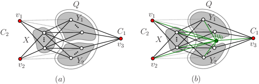
Figure 4.1: $(a)$ For $\kappa(G)=4k+2i$ with $i=0$, the graph attaining the lower bound of Theorem 4.4. $(b)$ For $\kappa(G)=4k+2i$ with $i=1$, the graph attaining the lower bound of Theorem 4.4.

Kriesell [61] obtained a result on the Steiner tree packing problem: Let $t\geq 1$ be a natural number and $G$ a graph, and let $\{a,b,c\}\subseteq V(G)$ be $\lfloor\frac{8t+3}{6}\rfloor$-edge-connected in $G$. Then there exists a system of $t$ edge-disjoint $\{a,b,c\}$-spanning trees. Using his result, Li, Mao and Sun derived a sharp lower bound of $\lambda_{3}(G)$ and gave graphs attaining the bound. With this lower bound, they got some results for line graphs (see Section $7$) and planar graphs.

Proposition 4.5

[88] Let $G$ be a connected graph with $n$ vertices. For every two integers $s$ and $r$ with $s\geq 0$ and $r\in\{0,1,2,3\}$, if $\lambda(G)=4s+r$, then $\lambda_{3}(G)\geq 3s+\lceil\frac{r}{2}\rceil$. Moreover, the lower bound is sharp. We simply write $\lambda_{3}(G)\geq\frac{3\lambda-2}{4}$.

They gave the following graph class to show that the lower bound is sharp.

Example 4.2. For $\lambda=4s$ with $s\geq 1$, let $P=X_{1}\cup X_{2}$ and $Q=Y_{1}\cup Y_{2}$ be two cliques with $|X_{1}|=|Y_{1}|=2s$ and $|X_{2}|=|Y_{2}|=2s$. Let $x,y$ be adjacent to every vertex in $P,Q$, respectively, and $z$ be adjacent to every vertex in $X_{1}$ and $Y_{1}$. Finally, they finished the construction of $G$ by adding a perfect matching between $X_{2}$ and $Y_{2}$. It can be checked that $\lambda=4s$ and $\lambda(S)\geq 3s$. One can also check that for other three vertices of $G$ the number of edge-disjoint trees connecting them is not less than $3s$. So, $\lambda_{3}(G)=3s$ and the graph $G$ attains the lower bound.

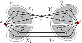
Figure 4.2: The graph with $\lambda(G)=4s$ and $\lambda_{3}(G)=3s$ that attains the lower bound of Proposition 4.5.

For $\lambda=4s+1$, let $|X_{1}|=|Y_{1}|=2s+1$ and $|X_{2}|=|Y_{2}|=2s$; for $\lambda=4s+2$, let $|X_{1}|=|Y_{1}|=2s+1$ and $|X_{2}|=|Y_{2}|=2s+1$; for $\lambda=4s+3$, let $|X_{1}|=|Y_{1}|=2s+2$ and $|X_{2}|=|Y_{2}|=2s+1$, where $s\geq 1$. Similarly, one can check that $\lambda_{3}(G)=3s+1$ for $\lambda=4s+1$; $\lambda_{3}(G)=3s+1$ for $\lambda=4s+2$; $\lambda_{3}(G)=3s+2$ for $\lambda=4s+3$.

For the case $s=0$, $G=P_{n}$ satisfies that $\lambda(G)=\lambda_{3}(G)=1$; $G=C_{n}$ satisfies that $\lambda(G)=2$ and $\lambda_{3}(G)=1$; $G=H_{t}$ satisfies that $\lambda(G)=3$ and $\lambda_{3}(G)=2$, where $H_{t}$ denotes the graph obtained from $t$ copies of $K_{4}$ by identifying a vertex from each of them in the way shown in Figure $4.3$.

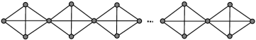
Figure 4.3: The graph $H_{t}$ with $\lambda(H_{t})=3,\lambda_{3}(H_{t})=2$.

Li, Mao and Sun gave a sharp upper bound of $\lambda_{k}(G)$.

Proposition 4.6

[88] For any graph $G$ of order $n$, $\lambda_{k}(G)\leq\lambda(G)$. Moreover, the upper bound is sharp.

But, for $\kappa_{k}(G)$, Li [77] only proved that $\kappa_{k}(G)\leq\kappa(G)$ for $3\leq k\leq 6$.

Theorem 4.7

[77] Let $G$ be a connected graph of order $n\geq 6$. Then for $3\leq k\leq 6$, $\kappa_{k}(G)\leq\kappa(G)$. Moreover, the upper bound is always sharp for $3\leq k\leq 6$.

A natural question is why $\kappa_{k}(G)\leq\kappa(G)$ is not true for $k\geq 6$ ? One may want to solve this problem by proving $\kappa_{k}(G)\leq\kappa_{k-1}(G)$ for $3\leq k\leq n$, namely, considering whether $\kappa_{k}$ is monotonically decreasing in $k$. Unfortunately, Li found a counterexample $G$ such that $\kappa_{4}(G)\geq\kappa_{3}(G)$. See the graph $G$ shown in Figure $4.1$ $(a)$ for $i=1$. Li showed that $\kappa(G)=4k+2$ and $\kappa_{3}(G)=3k+1$. It can be checked that the generalized $4$-connectivity $\kappa_{4}(G)=3k+2$, which means that $\kappa_{4}(G)\geq\kappa_{3}(G)$ for the graph $G$.

She also gave a graph $H(k,t)=(K_{\frac{k}{2}}\cup K_{\frac{k}{2}})\vee K_{t}$, where $k\geq 6$ and $t\geq 1$, to show that the monotone property of $\kappa_{k}$, namely, $\kappa_{n}\leq\kappa_{n-1}\leq\cdots\kappa_{4}\leq\kappa_{3}\leq\kappa$, is not true for $2\leq k\leq n$.

Proposition 4.8

[77] For any two integer $k\geq 6$ and $t\geq 1$, $\kappa_{k+2}(H(k+1,t))\geq\kappa_{k+1}(H(k,t))$.

However, for cubic graphs the conclusion holds.

Theorem 4.9

[77] If $G$ is a cubic graph, then $\kappa_{k}(G)\leq\kappa_{k-1}(G)$ for $3\leq k\leq n$.

Li and Mao [84] showed that the monotone property of $\lambda_{k}$ is true for $2\leq k\leq n$ although it is not true for $\kappa_{k}$.

Proposition 4.10

[84] For two integers $k$ and $n$ with $2\leq k\leq n-1$, and a connected graph $G$, we have $\lambda_{k+1}(G)\leq\lambda_{k}(G)$.

From Observation 2.1, we know that $\kappa_{k}(G)\leq\lambda_{k}(G)\leq\delta$. Actually, Li, Mao and Sun [88] showed that the graph $G=K_{k}\vee(n-k)K_{1}\ (n\geq 3k)$ satisfies that $\kappa_{k}(G)=\lambda_{k}(G)=\kappa(G)=\lambda(G)=\delta(G)=k$, which implies that the upper bounds of Observation 2.1, Proposition 4.6 and Theorem 4.7 are sharp.

Li and Mao [87] gave a sufficient condition for $\lambda_{k}(G)\leq\delta-1$. Li [77] obtained similar results on the generalized $k$-connectivity.

Proposition 4.11

[87] Let $G$ be a connected graph of order $n$ with minimum degree $\delta$. If there are two adjacent vertices of degree $\delta$, then $\lambda_{k}(G)\leq\delta-1$ for $3\leq k\leq n$. Moreover, the upper bound is sharp.

Proposition 4.12

[77] Let $G$ be a connected graph of order $n$ with minimum degree $\delta$. If there are two adjacent vertices of degree $\delta$, then $\kappa_{k}(G)\leq\delta-1$ for $3\leq k\leq n$. Moreover, the upper bound is sharp.

With the above bounds, we will focus on their applications. From Theorems 4.4 and 4.7, Li, Li and Zhou derived sharp bounds for planar graphs.

Theorem 4.13

[82] If $G$ is a connected planar graph, then $\kappa(G)-1\leq\kappa_{3}(G)\leq\kappa(G)$.

Motivated by constructing graphs to show that the upper and lower bounds are sharp, they obtained some lemmas. By the well-known Kuratowski’s theorem [20], they verified the following lemma.

Lemma 4.14

[82] For a connected planar graph $G$ with $\kappa_{3}(G)=k$, there are no $3$ vertices of degree $k$ in $G$, where $k\geq 3$.

They also studied the generalized $3$-connectivity of four kinds of graphs.

Lemma 4.15

[82] If $\kappa(G)\geq 3$, then $\kappa_{3}(G-e)\geq 2$ for any edge $e\in E(G)$.

Lemma 4.16

[82] If $G$ is a planar minimally $3$-connected graph, then $\kappa_{3}(G)=2$.

Lemma 4.17

[82] Let $G$ be a $4$-connected graph and let $H$ be a graph obtained from $G$ by adding a new vertex $w$ and jointing it to $3$ vertices of $G$. Then $\kappa_{3}(H)=\kappa(H)=3$.

Lemma 4.18

[82] If $G$ is a planar minimally $4$-connected graph, then $\kappa_{3}(H)=3$.

If $G$ is a connected planar graph, then $1\leq\kappa(G)\leq 5$ by Theorem 4.13. Then, for each $1\leq\kappa(G)\leq 5$, they gave some classes of planar graphs attaining the bounds of $\kappa_{3}(G)$, respectively.

Case 1: $\kappa(G)=1$. For any graph $G$ with $\kappa(G)=1$, obviously $\kappa_{3}(G)\geq 1$ and so $\kappa_{3}(G)=\kappa(G)=1$. Therefore, all planar graphs with connectivity $1$ can attain the upper bound, but can not attain the lower bound.

Case 2: $\kappa(G)=2$. Let $G$ be a planar graph with $\kappa(G)=2$ and having two adjacent vertices of degree $2$. Then by Theorem 4.13 $\kappa_{3}(G)\leq 1$ and so $\kappa_{3}(G)=1=\kappa(G)-1$. Therefore, this class of graphs attain the lower bound.

Let $G$ be a planar minimally $3$-connected graph. By the definition, for any edge $e\in E(G)$, $\kappa_{3}(G-e)=2$. Then by Lemma 4.15, it follows that $\kappa_{3}(G-e)=2$. Therefore, the $2$-connected planar graph $G-e$ attains the upper bound.

Case 3: $\kappa(G)=3$. For any planar minimally $3$-connected graph $G$, we know that $\kappa(G)=3$ and by Lemma 4.16, $\kappa_{3}(G)=2=\kappa(G)-1$. So this class of graphs attain the lower bound.

Let $G$ be a planar $4$-connected graph and let $H$ be a graph obtained from $G$ by adding a new vertex $w$ in the interior of a face for some planar embedding of $G$ and joining it to $3$ vertices on the boundary of the face. Then $H$ is still planar and by Lemma 4.17, one can immediately get that $\kappa_{3}(H)=\kappa(H)=3$, which means that $H$ attains the upper bound.

Figure 4.4: The graphs for the upper bound of Case $4$.

Case 4: $\kappa(G)=4$. For any planar minimally $4$-connected graph $G$, one knows that $\kappa(G)=4$, and by Lemma 4.18, $\kappa_{3}(G)=3=\kappa(G)-1$. So this class of graphs attain the lower bound.

For every graph in Figure $4.4$, the vertex in the center has degree $4$ and it can be checked that for any $2$ vertices there always exist four pairwise internally disjoint paths connecting them, which means that $\kappa(G)=4$. It can also be checked that for any $3$ vertices there always exist four pairwise internally disjoint trees connecting them. Combining this with Theorem 4.13, one can get that $\kappa_{3}(G)=4$. Therefore, the graphs attain the upper bound. Moreover, we can construct a series of graphs according to the pattern of Figure $4.4$, which attain the upper bound.

Case 5: $\kappa(G)=5$. For any planar graph $G$ with $\kappa(G)=5$, by Lemma 4.14 one can get that $\kappa_{3}(G)=4$. So, any planar graph $G$ with connectivity $5$ can attain the lower bound, but obviously can not attain the upper bound.

Similarly, the following result is obvious from Propositions 4.5 and 4.6.

Proposition 4.19

[88] If $G$ be a connected planar graph, then $\lambda(G)-1\leq\lambda_{3}(G)\leq\lambda(G)$.

5 Graphs with given generalized (edge-)connectivity

From the last section, we know that $1\leq\kappa_{k}(G)\leq n-\lceil k/2\rceil$ and $1\leq\lambda_{k}(G)\leq n-\lceil k/2\rceil$ for a connected graph $G$. Li, Mao and Sun [88] considered to characterize graphs attaining the upper bounds, namely, graphs with $\kappa_{k}(G)=n-\lceil k/2\rceil$ or $\lambda_{k}(G)=n-\lceil k/2\rceil$. Since a complete graph $K_{n}$ possesses the maximum generalized (edge-)connectivity, they wanted to find out the critical value of the number of edges, denoted by $\mathbbm{t}$, such that the generalized (edge-)connectivity of the resulting graph will keep being $n-\lceil k/2\rceil$ by deleting $\mathbbm{t}$ edges from a complete graph $K_{n}$ but will not keep being $n-\lceil k/2\rceil$ by deleting $\mathbbm{t}+1$ edges. By further investigation, they conjectured that $\mathbbm{t}$ may be $0$ for $k$ even and $\frac{k-1}{2}$ for $k$ odd.

First, they noticed that for arbitrary $S\subseteq V(G)$ there are two types of edge-disjoint trees connecting $S$: A tree of Type $I$ is a tree whose edges all belong to $E(G[S])$; a tree of Type $II$ is a tree containing at least one edge of $E_{G}[S,\bar{S}]$. We denote the set of the edge-disjoint trees of Type $I$ and Type $II$ by $\mathscr{T}_{1}$ and $\mathscr{T}_{2}$, respectively. Let $\mathscr{T}=\mathscr{T}_{1}\cup\mathscr{T}_{2}$.

Lemma 5.1

[88] Let $S\subseteq V(G)$, $|S|=k$ and $T$ be a tree connecting $S$. If $T\in\mathscr{T}_{1}$, then $T$ uses $k-1$ edges of $E(G[S])\cup E_{G}[S,\bar{S}]$; If $T\in\mathscr{T}_{2}$, then $T$ uses at least $k$ edges of $E(G[S])\cup E_{G}[S,\bar{S}]$.

5.1 Graphs with $\kappa_{k}(G)=n-\lceil\frac{k}{2}\rceil$ and $\lambda_{k}(G)=n-\lceil\frac{k}{2}\rceil$

They found that $|E(G[S])\cup E_{G}[S,\bar{S}]|$ is fixed once the graph $G$ is given whatever there exist how many trees of Type $I$ and how many trees of Type $II$. From Lemma 5.1, each tree will use certain number of edges in $E(G[S])\cup E_{G}[S,\bar{S}]$. Deleting excessive edges from a complete graph $K_{n}$ will result in that the remaining edges in $E(G[S])\cup E_{G}[S,\bar{S}]$ will not form $n-\lceil k/2\rceil$ trees. By using such an idea, they proved that $\lambda_{k}(G)<n-\lceil\frac{k}{2}\rceil$ for $\mathbbm{t}\geq 1$ ($k$ is even) and $\lambda_{k}(G)<n-\lceil\frac{k}{2}\rceil$ for $\mathbbm{t}\geq\frac{k+1}{2}$ ($k$ is odd). Furthermore, from Observation 2.1, $\kappa_{k}(G)<n-\lceil\frac{k}{2}\rceil$ for $\mathbbm{t}\geq 1$ ($k$ is even) and $\kappa_{k}(G)<n-\lceil\frac{k}{2}\rceil$ for $\mathbbm{t}\geq\frac{k+1}{2}$ ($k$ is odd).

Next, they only needed to find out $n-\lceil k/2\rceil$ internally disjoint trees connecting $S$ in $G$, where $G=K_{n}$ for $k$ even; $G=K_{n}\setminus M$ and $M$ is an edge set such that $|M|=\frac{k-1}{2}$ for $k$ odd. Obviously, it only needs to consider the case that $k$ is odd. But the difficulty is that each edge of $E(G[S])\cup E_{G}[S,\bar{S}]$ belongs to a tree connecting $S$ and can not be wasted. Fortunately, Nash-Williams-Tutte theorem provides a perfect solution. They first derived the following lemma from Theorem 1.3.

Lemma 5.2

[88] If $n$ is odd and $M$ is an edge set of the complete graph $K_{n}$ such that $0\leq|M|\leq\frac{n-1}{2}$, then $G=K_{n}\setminus M$ contains $\frac{n-1}{2}$ edge-disjoint spanning trees.

They wanted to find out $\frac{k-1}{2}$ edge-disjoint spanning trees in $G[S]$ (By the definition of internally disjoint trees, these trees are internally disjoint trees connecting $S$, as required). Then their basic idea is to seek for some edges in $G[S]$, and let them together with the edges of $E_{G}[S,\bar{S}]$ form $n-k$ internally disjoint trees. They proved that there are indeed $n-k$ internally disjoint trees in the premise that $G[S]$ contains $\frac{k-1}{2}$ edge-disjoint spanning trees. Actually, Lemma 5.2 can guarantee the existence of such $\frac{k-1}{2}$ trees. Then they found out $n-\frac{k-1}{2}$ internally disjoint trees connecting $S$ and accomplished the proof of the following theorem.

Theorem 5.3

[88] Let $k,n$ be two integers with $2\leq k\leq n$. Then for a connected graph $G$ of order $n$, $\kappa_{k}(G)=n-\lceil\frac{k}{2}\rceil$ if and only if $G=K_{n}$ for $k$ even; $G=K_{n}\setminus M$ for $k$ odd, where $M$ is an edge set such that $0\leq|M|\leq\frac{k-1}{2}$.

Combining Theorem 5.3 and Observation 2.1, they obtained the following theorem for $\lambda_{k}(G)$.

Theorem 5.4

[88] Let $k,n$ be two integers with $2\leq k\leq n$. Then for a connected graph $G$ of order $n$, $\lambda_{k}(G)=n-\lceil\frac{k}{2}\rceil$ if and only if $G=K_{n}$ for $k$ even; $G=K_{n}\setminus M$ for $k$ odd, where $M$ is an edge set such that $0\leq|M|\leq\frac{k-1}{2}$.

5.2 Graphs with $\kappa_{k}(G)=n-\lceil\frac{k}{2}\rceil-1$ and $\lambda_{k}(G)=n-\lceil\frac{k}{2}\rceil-1$

As a continuation of their investigation, Li and Mao later turned their attention to characterizing graphs $G$ with $\kappa_{k}(G)=n-\lceil\frac{k}{2}\rceil-1$ and $\lambda_{k}(G)=n-\lceil\frac{k}{2}\rceil-1$. One may notice that $\kappa_{k}(G)=n-\lceil\frac{k}{2}\rceil$ if and only if $G$ itself is the complete graph $K_{n}$ for $k$ even. So for $k$ even it is possible to continue to characterize $\kappa_{k}(G)=n-\lceil\frac{k}{2}\rceil-1$ by deleting more edges from the complete graph $K_{n}$.

Theorem 5.5

[89] Let $n$ and $k$ be two integers such that $k$ is even and $4\leq k\leq n$, and $G$ be a connected graph of order $n$. Then $\kappa_{k}(G)=n-\frac{k}{2}-1$ if and only if $G=K_{n}\setminus M$ where $M$ is an edge set such that $1\leq\Delta(K_{n}[M])\leq\frac{k}{2}$ and $1\leq|M|\leq k-1$.

Different from the proof of Theorem 5.3, in order to find $n-\frac{k}{2}-1$ internally disjoint trees in $G[S]\cup G[S,\bar{S}]$, they designed a procedure to emphasize seeking for some edges “evenly” in $G[S]$, and let them together with the edges of $E_{G}[S,\bar{S}]$ form $n-k$ internally disjoint trees $T_{1},T_{2},\cdots,T_{n-k}$ with its root $w_{1},w_{2},\cdots,w_{n-k}\in\bar{S}$, respectively. Applying this procedure designed by them, they proved that the remaining edges in $G[S]$ can form $\frac{k-2}{2}$ spanning trees, which are also $\frac{k-2}{2}$ internally disjoint trees connecting $S$. These trees together with $T_{1},T_{2},\cdots,T_{n-k}$ are $n-\frac{k}{2}-1$ internally disjoint trees connecting $S$, accomplishing the proof of the above theorem.

With the help of Theorem 5.5 and Observation 2.1, they obtained the following theorem for $\lambda_{k}(G)$.

Theorem 5.6

[89] Let $n$ and $k$ be two integers such that $k$ is even and $2\leq k\leq n$, and $G$ be a connected graph of order $n$. Then $\lambda_{k}(G)=n-\frac{k}{2}-1$ if and only if $G=K_{n}\setminus M$ where $M$ is an edge set satisfying one of the following conditions:

$(1)$ $\Delta(K_{n}[M])=1$ and $1\leq|M|\leq\lfloor\frac{n}{2}\rfloor$;

$(2)$ $2\leq\Delta(K_{n}[M])\leq\frac{k}{2}$ and $1\leq|M|\leq k-1$.

By Nash-Williams-Tutte theorem, they luckily characterized the graphs attaining the upper bound and graphs with $\kappa_{k}(G)=n-\lceil\frac{k}{2}\rceil-1$ and $\kappa_{k}(G)=n-\lceil\frac{k}{2}\rceil-1$ for $k$ even. But, for $k$ odd, it is not easy to characterize the graphs with $\kappa_{k}(G)=n-\lceil\frac{k}{2}\rceil-1$. So, Li, Li, Mao and Sun considered the case $k=3$, namely, they considered graphs with $\kappa_{3}(G)=n-3$.

Theorem 5.7

[74] Let $G$ be a connected graph of order $n\ (n\geq 3)$. Then $\kappa_{3}(G)=n-3$ if and only if $G$ is a graph obtained from the complete graph $K_{n}$ by deleting an edge set $M$ such that $K_{n}[M]=P_{4}$ or $K_{n}[M]=P_{3}\cup rP_{2}\ (r=1,2)$ or $K_{n}[M]=C_{3}\cup rP_{2}\ (r=1,2)$ or $K_{n}[M]=sP_{2}\ (2\leq s\leq\lfloor\frac{n}{2}\rfloor)$.

But, for the edge case, Li and Mao [87] showed that the statement is different.

Theorem 5.8

[87] Let $G$ be a connected graph of order $n$. Then $\lambda_{3}(G)=n-3$ if and only if $G$ is a graph obtained from the complete graph $K_{n}$ by deleting an edge set $M$ such that $K_{n}[M]=rP_{2}\ (2\leq r\leq\lfloor\frac{n}{2}\rfloor)$ or $K_{n}[M]=P_{4}\cup sP_{2}\ (0\leq s\leq\lfloor\frac{n-4}{2}\rfloor)$ or $K_{n}[M]=P_{3}\cup tP_{2}\ (0\leq t\leq\lfloor\frac{n-3}{2}\rfloor)$ or $K_{n}[M]=C_{3}\cup tP_{2}\ (0\leq t\leq\lfloor\frac{n-3}{2}\rfloor)$.

6 Nordhaus-Gaddum-type results

Let $\mathcal{G}(n)$ denote the class of simple graphs of order $n$ and $\mathcal{G}(n,m)$ the subclass of $\mathcal{G}(n)$ having graphs with $n$ vertices and $m$ edges. Give a graph parameter $f(G)$ and a positive integer $n$, the Nordhaus-Gaddum (N-G) Problem is to determine sharp bounds for: $(1)$ $f(G)+f(\overline{G})$ and $(2)$ $f(G)\cdot f(\overline{G})$, as $G$ ranges over the class $\mathcal{G}(n)$, and characterize the extremal graphs. The Nordhaus-Gaddum type relations have received wide attention; see a recent survey paper [4] by Aouchiche and Hansen.

Alavi and Mitchem in [3] investigated Nordhaus-Gaddum-type results for the classical connectivity and edge-connectivity in $\mathcal{G}(n)$. Achuthan and Achuthan [1] considered the same problem in $\mathcal{G}(n,m)$.

6.1 Results for graphs in $\mathcal{G}(n)$

Li and Mao [84] investigated the Nordhaus-Gaddum type relations on the generalized edge-connectivity. At first, they focused on the graphs in $\mathcal{G}(n)$.

Theorem 6.1

[84] Let $G\in\mathcal{G}(n)$, and $k,n$ be two integers with $2\leq k\leq n$. Then

$(1)$ $1\leq\lambda_{k}(G)+\lambda_{k}(\overline{G})\leq n-\lceil k/2\rceil$;

$(2)$ $0\leq\lambda_{k}(G)\cdot\lambda_{k}(\overline{G})\leq\big{[}\frac{n-\lceil k/2\rceil}{2}\big{]}^{2}$.

Moreover, the upper and lower bounds are sharp.

The following observation indicates the graphs attaining the above lower bound.

Observation 6.2

[84] $\lambda_{k}(G)\cdot\lambda_{k}(\overline{G})=0$ if and only if $G$ or $\overline{G}$ is disconnected.

For $n\geq 5$, $\mathcal{G}_{n}^{1}$ is a graph class as shown in Figure 6.1 $(a)$ such that $\lambda(G)=1$ and $d_{G}(v_{1})=n-1$ for $G\in\mathcal{G}_{n}^{1}$, where $v_{1}\in V(G)$; $\mathcal{G}_{n}^{2}$ is a graph class as shown in Figure 6.1 $(b)$ such that $\lambda(G)=2$ and $d_{G}(u_{1})=n-1$ for $G\in\mathcal{G}_{n}^{2}$, where $u_{1}\in V(G)$; $\mathcal{G}_{n}^{3}$ is a graph class as shown in Figure 6.1 $(c)$ such that $\lambda(G)=2$ and $d_{G}(v_{1})=n-1$ for $G\in\mathcal{G}_{n}^{3}$, where $v_{1}\in V(G)$; $\mathcal{G}_{n}^{4}$ is a graph class as shown in Figure 6.1 $(d)$ such that $\lambda(G)=2$.

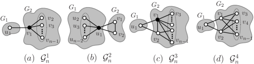
Figure 6.1: The graph classes $\mathcal{G}_{n}^{i}\ (1\leq i\leq 4)$

As we know, it is not easy to characterize the graphs with $\lambda_{k}(G)=1$, even with $\lambda_{3}(G)=1$. So, Li and Mao wanted to add some conditions to attack such a problem. Motivated by such an idea, they hope to characterize the graphs with $\lambda_{k}(G)+\lambda_{k}(\overline{G})=1$. Actually, the Norhaus-Gaddum-type problems also need to characterize the extremal graphs attaining the bounds.

Proposition 6.3

[84] $\lambda_{k}(G)+\lambda_{k}(\overline{G})=1$ if and only if $G$ (symmetrically, $\overline{G}$) satisfies one of the following conditions:

$\bullet$ $G\in\mathcal{G}_{n}^{1}$ or $G\in\mathcal{G}_{n}^{2}$;

$\bullet$ $G\in\mathcal{G}_{n}^{3}$ and there exists a component $G_{i}$ of $G\setminus v_{1}$ such that $G_{i}$ is a tree and $|V(G_{i})|<k$;

$\bullet$ $G\in\{P_{3},C_{3}\}$ for $k=n=3$, or $G\in\{C_{4},K_{4}\setminus e\}$ for $k=n=4$, or $G=K_{3,3}$ for $k=n=6$, or $G=K_{2,n-2}$ for $k=n-1$ and $n\geq 5$, or $G=C_{4}$ for $k=n-1=3$, or $G\in\{K_{2,n-2}^{+},K_{2,n-2}\}$ for $k=n$ and $n\geq 5$ where $K_{2,n-2}^{+}$ denote the graph obtained from the complete bipartite graph $K_{2,n-2}$ by adding one edge in the part with $n-2$ vertices.

Let us focus on $(1)$ of Theorem 6.1. If one of $G$ and $\overline{G}$ is disconnected, we can characterize the graphs attaining the upper bound by Theorem 5.4.

Proposition 6.4

[84] For any graph $G$ of order $n$, if $G$ is disconnected, then $\lambda_{k}(G)+\lambda_{k}(\overline{G})=n-\lceil\frac{k}{2}\rceil$ if and only if $\overline{G}=K_{n}$ for $k$ even; $\overline{G}=K_{n}\setminus M$ for $k$ odd, where $M$ is an edge set such that $0\leq|M|\leq\frac{k-1}{2}$.

If both $G$ and $\overline{G}$ are connected, we can obtain a structural property of the graphs attaining the upper bound although it seems too difficult to characterize them.

Proposition 6.5

[84] If $\lambda_{k}(G)+\lambda_{k}(\overline{G})=n-\lceil\frac{k}{2}\rceil$, then $\Delta(G)-\delta(G)\leq\lceil\frac{k}{2}\rceil-1$.

One can see that the graphs with $\lambda_{k}(G)+\lambda_{k}(\overline{G})=n-\lceil\frac{k}{2}\rceil$ must have a uniform degree distribution. By this property, Li and Mao constructed a graph class to show that the two upper bounds of Theorem 6.1 are tight for $k=n$.

Example 6.1.  Let $n,r$ be two positive integers such that $n=4r+1$. From Theorem 2.5, we know that $\kappa_{n}(K_{2r,2r+1})=\lambda_{n}(K_{2r,2r+1})=r$. Let $\mathcal{E}$ be the set of the edges of these $r$ spanning trees in $K_{2r,2r+1}$. Then there exist $2r(2r+1)-4r^{2}=2r$ remaining edges in $K_{2r,2r+1}$ except for the edges in $\mathcal{E}$. Let $M$ be the set of these $2r$ edges. Set $G=K_{2r,2r+1}\setminus M$. Then $\lambda_{n}(G)=r$, $M\subseteq E(\overline{G})$ and $\overline{G}$ is a graph obtained from two cliques $K_{2r}$ and $K_{2r+1}$ by adding $2r$ edges in $M$ between them, that is, one endpoint of each edge belongs to $K_{2r}$ and the other endpoint belongs to $K_{2r+1}$. Note that $E(\overline{G})=E(K_{2r})\cup M\cup E(K_{2r+1})$. Now we show that $\lambda_{n}(\overline{G})\geq r$. As we know, $K_{2r}$ contains $r$ Hamiltonian paths, say $P_{1},P_{2},\cdots,P_{r}$, and so does $K_{2r+1}$, say $P_{1}^{\prime},P_{2}^{\prime},\cdots,P_{r}^{\prime}$. Pick up $r$ edges from $M$, say $e_{1},e_{2},\cdots,e_{r}$, let $T_{i}=P_{i}\cup P_{i}^{\prime}\cup e_{i}(1\leq i\leq r)$. Then $T_{1},T_{2},\cdots,T_{r}$ are $r$ spanning trees in $\overline{G}$, namely, $\lambda_{n}(\overline{G})\geq r$. Since $|E(\overline{G})|={{2r}\choose{2}}+{{2r+1}\choose{2}}+2r=4r^{2}+2r$ and each spanning tree uses $4r$ edges, these edges can form at most $\lfloor\frac{4r^{2}+2r}{4r}\rfloor=r$ spanning trees, that is, $\lambda_{n}(\overline{G})\leq r$. So $\lambda_{n}(\overline{G})=r$. Clearly, $\lambda_{n}(G)+\lambda_{n}(\overline{G})=2r=\frac{n-1}{2}=n-\lceil\frac{n}{2}\rceil$ and $\lambda_{n}(\overline{G})\cdot\lambda_{n}(\overline{G})=r^{2}=\big{[}\frac{n-\lceil n/2\rceil}{2}\big{]}^{2}$.

Li, Mao and Sun [88] were concerned with analogous inequalities involving the generalized $k$-connectivity for the graphs in $\mathcal{G}(n)$.

Theorem 6.6

[88] Let $G\in\mathcal{G}(n)$, and $k,n$ be two integers with $2\leq k\leq n$. Then

$(1)$ $1\leq\kappa_{k}(G)+\kappa_{k}(\overline{G})\leq n-\lceil k/2\rceil$;

$(2)$ $0\leq\kappa_{k}(G)\cdot\kappa_{k}(\overline{G})\leq[\frac{2n-\lceil k\rceil}{4}]^{2}$.

Moreover, the upper and lower bounds are sharp.

6.2 Results for graphs in $\mathcal{G}(n,m)$

Then, Li and Mao also focused on the graphs in $\mathcal{G}(n,m)$ in [84]. Let us begin with another problem, called the maximum connectivity of a graph. It was pointed out by Harary [53] that given the number of vertices and edges of a graph, the largest connectivity possible can also be read out of the inequality $\kappa(G)\leq\lambda(G)\leq\delta(G)$.

Theorem 6.7

[53] For each pair of integers $n,m$ with $0\leq n-1\leq m\leq{{n}\choose{2}}$,

$$\kappa(G)\leq\lambda(G)\leq\Big{\lfloor}\frac{2m}{n}\Big{\rfloor},$$

where the maximum is taken over all graphs $G\in\mathcal{G}(n,m)$.

Li and Mao considered the similar problem for the generalized edge-connectivity.

Corollary 6.8

[84] For any graph $G\in\mathcal{G}(n,m)$ and $3\leq k\leq n$, $\lambda_{k}(G)=0$ for $m<n-1$; $\lambda_{k}(G)\leq\lfloor\frac{2m}{n}\rfloor$ for $m\geq n-1$.

Although the above bound of $\lambda_{k}(G)$ is the same as $\lambda(G)$, the graphs attaining the upper bound seems to be very rare. Actually, we can obtain some structural properties of these graphs.

Proposition 6.9

[84] For any $G\in\mathcal{G}(n,m)$ and $3\leq k\leq n$, if $\lambda_{k}(G)=\lfloor\frac{2m}{n}\rfloor$ for $m\geq n-1$, then

$\bullet$ $\frac{2m}{n}$ is not an integer;

$\bullet$ $\delta(G)=\lfloor\frac{2m}{n}\rfloor$;

$\bullet$ for $u,v\in V(G)$ such that $d_{G}(u)=d_{G}(v)=\lfloor\frac{2m}{n}\rfloor$, $uv\notin E(G)$.

By Theorem 1.3 and Corollary 6.8, they derived the following theorem.

Theorem 6.10

[84] Let $G\in\mathcal{G}(n,m)$. For $n\geq 6$, we have

$(1)$ $L(n,m)\leq\lambda_{k}(G)+\lambda_{k}(\overline{G})\leq M(n,m)$;

$(2)$ $0\leq\lambda_{k}(G)\cdot\lambda_{k}(\overline{G})\leq N(n,m)$,

where

$$L(n,m)=\left\{\begin{array}[]{ll}max\{1,\lfloor\frac{1}{2}(n-2-m)\rfloor\},&if~{}\lfloor\frac{n}{3}\rfloor+1\leq m\leq{{n}\choose{2}};\\ min\{n-2m-1,\lfloor\frac{n}{2}-\frac{2m}{n-1}\rfloor\},&if~{}0\leq m\leq\lfloor\frac{n}{3}\rfloor.\end{array}\right.$$

$$M(n,m)=\left\{\begin{array}[]{ll}n-\lceil\frac{k}{2}\rceil,&if~{}m\geq n-1,\\ &~{}or~{}k~{}is~{}even~{}and~{}m=0,\\ &~{}or~{}k~{}is~{}odd~{}and~{}0\leq m\leq\frac{k-1}{2};\\ n-\lceil\frac{k}{2}\rceil-1,&if~{}k~{}is~{}even~{}and~{}1\leq m<n-1,\\ &~{}or~{}k~{}is~{}odd~{}and~{}\frac{k+1}{2}\leq m<n-1.\end{array}\right.$$

$$N(n,m)=\left\{\begin{array}[]{ll}0,&if~{}0\leq m\leq n-2;\\ (\frac{2m}{n}-1)(n-2-\frac{2m}{n}),&if~{}m\geq n-1~{}and~{}2m\equiv 0(mod~{}n);\\ \lfloor\frac{2m}{n}\rfloor(n-2-\lfloor\frac{2m}{n}\rfloor),&otherwise.\end{array}\right.$$

Moreover, the upper and lower bounds are sharp.

7 Results for graph operations

In this section we will survey the results for line graphs and graph products.

7.1 Results for line graphs

Chartrand and Steeart [25] investigated the relation between the connectivity and edge-connectivity of a graph and its line graph. They proved that if $G$ is a connected graph, then $(1)$ $\kappa(L(G))\geq\lambda(G)$ if $\lambda(G)\geq 2$; $(2)$ $\lambda(L(G))\geq 2\lambda(G)-2$; $(3)$ $\kappa(L(L(G)))\geq 2\kappa(G)-2$. With the help of Proposition 4.5, Li, Mao and Sun also considered the generalized $3$-connectivity and $3$-edge-connectivity for line graphs.

Proposition 7.1

[88] If $G$ is a connected graph, then

$(1)$ $\lambda_{3}(G)\leq\kappa_{3}(L(G))$.

$(2)$ $\lambda_{3}(L(G))\geq\frac{3}{2}\lambda_{3}(G)-2$.

$(3)$ $\kappa_{3}(L(L(G))\geq\frac{3}{2}\kappa_{3}(G)-2$.

First, they proved $(1)$ of this theorem. Next, combining Proposition 4.5 with $(1)$ of Proposition 7.1, they derived $(2)$ and $(3)$ of Proposition 7.1. One can check that $(1)$ of this proposition is sharp since $G=C_{n}$ can attain this bound.

Let $L^{0}(G)=G$ and $L^{1}(G)=L(G)$. Then for $r\geq 2$, the $r$-$th$ iterated line graph $L^{r}(G)$ of $G$ is defined by $L(L^{r-1}(G))$. The next statement follows immediately from Proposition 7.1 and a routine application of induction.

Corollary 7.2

[88] $\lambda_{3}(L^{r}(G))\geq(\frac{3}{2})^{r}(\lambda_{3}(G)-4)+4$, and $\kappa_{3}(L^{r}(G))\geq(\frac{3}{2})^{\lfloor\frac{r}{2}\rfloor}(\kappa_{3}(G)-4)+4$.

7.2 Results for graph products

Product networks were proposed based upon the idea of using the cross product as a tool for “combining” two known graphs with established properties to obtain a new one that inherits properties from both [31]. Recently, there has been an increasing interest in a class of interconnection networks called Cartesian product networks; see [6, 31, 64]. In [64], Ku, Wang and Hung studied the problem of constructing the maximum number of edge-disjoint spanning trees in Cartesian product networks, and gave a sharp lower bound of $\kappa_{n}(G\Box H)$.

Theorem 7.3

[64] For two connected graphs $G$ and $H$, $\kappa_{n}(G\Box H)\geq\kappa_{n}(G)+\kappa_{n}(H)-1$. Moreover, the lower bound is sharp.

But the upper bound of $\kappa_{n}(G\Box H)$ is still unknown. A natural question is to study the following problems:

$\bullet$ Give sharp upper and lower bounds of $\kappa_{k}(G*H)$, where $*$ is a kind of graph product.

$\bullet$ Give sharp upper and lower bounds of $\lambda_{k}(G*H)$, where $*$ is a kind of graph product.

Sabidussi in [117] derived a result on the classical connectivity of Cartesian product graphs: for two connected graphs $G$ and $H$, $\kappa(G\square H)\geq\kappa(G)+\kappa(H)$. But we mention that it was incorrectly claimed in ([52], page 308) that $\kappa(G\Box H)=\kappa(G)+\kappa(H)$ holds for any connected $G$ and $H$. In [120], S̆pacapan proved that $\kappa(G\Box H)=\min\{\kappa(G)|V(H)|,\kappa(H)|V(G)|,\delta(G)+\delta(H)\}$ for two nontrivial graphs $G$ and $H$.

7.2.1 The case $k=3$

In [76], Li, Li and Sun investigated the generalized $3$-connectivity of Cartesian product graphs. Their results could be seen as a generalization of Sabidussi’s result. As usual, in order to get a general result, they first began with a special case.

Proposition 7.4

[76] Let $G$ be a graph and $P_{m}$ be a path with $m$ edges. The following assertions hold:

$(1)$ If $\kappa_{3}(G)=\kappa(G)\geq 1$, then $\kappa_{3}(G\square P_{m})\geq\kappa_{3}(G)$. Moreover, the bound is sharp.

$(2)$ If $1\leq\kappa_{3}(G)<\kappa(G)$, then $\kappa_{3}(G\square P_{m})\geq\kappa_{3}(G)+1$. Moreover, the bound is sharp.

Note that $Q_{n}\cong P_{2}\square P_{2}\square\cdots\square P_{2}$, where $Q_{n}$ is the $n$-hypercube. They got the following corollary.

Corollary 7.5

[76] Let $Q_{n}$ be the $n$-hypercube with $n\geq 2$. Then $\kappa_{3}(Q_{n})=n-1$.

Example 4. Let $H_{1}$ and $H_{2}$ be two complete graphs of order $n$, and let $V(H_{1})=\{u_{1},u_{2},\cdots,$ $u_{n}\}$, $V(H_{2})=\{v_{1},v_{2},\cdots,v_{n}\}$. We now construct a graph $G$ as follows: $V(G)=V(H_{1})\cup V(H_{2})\cup\{w\}$ where $w$ is a new vertex; $E(G)=E(H_{1})\cup E(H_{2})\cup\{u_{i}v_{j}|1\leq i,j\leq n\}\cup\{wu_{i}|1\leq i\leq n\}$. It is easy to check that $\kappa_{3}(G\square K_{2})=\kappa_{3}(G)=n$.

They showed that the bounds of $(1)$ and $(2)$ in Proposition 7.4 are sharp by Example $4$ and Corollary 7.5.

Next, they studied the generalized $3$-connectivity of the Cartesian product of a graph $G$ and a tree $T$, which will be used in Theorem 7.7.

Proposition 7.6

[76] Let $G$ be a graph and $T$ be a tree. The following assertions hold:

$(1)$ If $\kappa_{3}(G)=\kappa(G)\geq 1$, then $\kappa_{3}(G\square T)\geq\kappa_{3}(G)$. Moreover, the bound is sharp.

$(2)$ If $1\leq\kappa_{3}(G)<\kappa(G)$, then $\kappa_{3}(G\square T)\geq\kappa_{3}(G)+1$. Moreover, the bound is sharp.

The bounds of $(1)$ and $(2)$ in Proposition 7.6 are sharp by Example $4$ and Corollary 7.5.

They mainly investigated the generalized $3$-connectivity of the Cartesian product of two connected graphs $G$ and $H$. By decomposing $H$ into some trees connecting $2$ vertices or $3$ vertices, they considered the Cartesian product of a graph $G$ and a tree $T$ and obtained Theorem 7.7 by Proposition 7.6.

Theorem 7.7

[76] Let $G$ and $H$ be connected graphs such that $\kappa_{3}(G)>\kappa_{3}(H)$. The following assertions hold:

$(1)$ If $\kappa(G)=\kappa_{3}(G)$, then $\kappa_{3}(G\square H)\geq\kappa_{3}(G)+\kappa_{3}(H)-1$. Moreover, the bound is sharp.

$(2)$ If $\kappa(G)>\kappa_{3}(G)$, then $\kappa_{3}(G\square H)\geq\kappa_{3}(G)+\kappa_{3}(H)$. Moreover, the bound is sharp.

They also showed that the bounds of $(1)$ and $(2)$ in Theorem 7.7 are sharp. Let $K_{n}$ be a complete graph with $n$ vertices, and $P_{m}$ be a path with $m$ vertices, where $m\geq 2$. Since $\kappa_{3}(P_{m})=1$ and $\kappa_{3}(K_{n})=n-2$, it is easy to see that $\kappa_{3}(K_{n}\square P_{m})=n-1$. Thus, $K_{n}\square P_{m}$ is a sharp example for $(1)$. For $(2)$, Example $4$ is a sharp one.

Lexicographic product is one of the standard products, which are studied extensively; see [52]. Recently, some applications in networks of the lexicographic product were studied; see [13, 36, 71]. Yang and Xu [129] investigated the classical connectivity of the lexicographic product of two graphs: For two graphs $G$ and $H$, if $G$ is non-trivial, non-complete and connected, then $\kappa(G\circ H)=\kappa(G)|V(H)|$.

Using Fan Lemma ([127], page 170) and Expansion Lemma ([127], page 162), Li and Mao [86] obtained the following lower bound of $\kappa_{3}(G\circ H)$, which could be seen as an extension of Yang and Xu’ result.

Theorem 7.8

[86] Let $G$ and $H$ be two connected graphs. Then

$$\kappa_{3}(G\circ H)\geq\kappa_{3}(G)|V(H)|.$$

Moreover, the bound is sharp.

For a tree $T$ and a connected graph $H$, they showed that $\kappa_{3}(T\circ H)=|V(H)|$, which can be seen as an improvement of Theorem 7.8. From Theorem 7.7, one may wonder whether $\kappa_{3}(T\Box H)=\kappa_{3}(T)+\kappa_{3}(H)-1$ for a connected graph $H$ and a tree $T$ (note that $\kappa_{3}(T)=\kappa(T)=1$). For example, let $T=P_{3}$ and $H=K_{4}$. Then $\kappa_{3}(T)=\kappa(T)=1$ and $\kappa_{3}(H)=2$. One can check that $\kappa_{3}(T\Box H)=3>2=\kappa_{3}(T)+\kappa_{3}(H)-1$. So the equality does not hold for the Cartesian product of a tree and a connected graph.

For the edge version of the above mentioned problem, Yang and Xu [129] also derived that $\lambda(G\circ H)=\min\{\lambda(G)|V(H)|^{2},\delta(H)+\delta(G)|V(H)|\}$ for a connected graph $G$ and a non-trivial graphs $H$. Recently, Li, Yue and Zhao [90] gave a lower bound of $\lambda_{3}(G\circ H)$.

Theorem 7.9

[90] Let $G$ and $H$ be a connected graph. Then

$$\lambda_{3}(G\circ H)\geq\lambda_{3}(H)+\lambda_{3}(G)|V(H)|.$$

Moreover, the lower bound is sharp.

From Theorems 4.4 and 4.7, and Yang and Xu’ s result, Li and Mao [86] derived a upper bound of $\kappa_{3}(G\circ H)$.

Theorem 7.10

[86] Let $G$ and $H$ be two connected graphs. If $G$ is non-trivial and non-complete, then $\kappa_{3}(G\circ H)\leq\lfloor\frac{4}{3}\kappa_{3}(G)+r-\frac{4}{3}\lceil\frac{r}{2}\rceil\rfloor|V(H)|$, where $r\equiv\kappa(G)\ (mod~{}4)$. Moreover, the bound is sharp.

The graph $P_{n}\circ P_{3}\ (n\geq 4)$ indicates that both the lower bound of Theorem 7.8 and the upper bound of Theorem 7.10 are sharp.

In the same paper, they also derived the following upper bound of $\kappa_{3}(G\Box H)$ from Theorems 4.4 and 4.7, and S̆pacapan’s result.

Theorem 7.11

[86] Let $G$ and $H$ be two connected graphs. Then $\kappa_{3}(G\Box H)\leq\min\{\lfloor\frac{4}{3}\kappa_{3}(G)+r_{1}-\frac{4}{3}\lceil\frac{r_{1}}{2}\rceil\rfloor|V(H)|,\lfloor\frac{4}{3}\kappa_{3}(H)+r_{2}-\frac{4}{3}\lceil\frac{r_{2}}{2}\rceil\rfloor|V(G)|,\delta(G)+\delta(H)\}$, where $r_{1}\equiv\kappa(G)\ (mod\ 4)$ and $r_{2}\equiv\kappa(H)\ (mod\ 4)$. Moreover, the bound is sharp.

The graph $P_{n}\circ P_{m}\ (n\geq 4,\ m\geq 4)$ is a sharp example for the above theorem.

In [90], Li, Yue and Zhao also obtained an upper bound of $\lambda_{3}(G\circ H)$.

Theorem 7.12

[90] Let $G$ be a connected graph, and $H$ be a non-trivial graph. Then $\lambda_{3}(G\circ H)\leq\min\{\lfloor\frac{4\lambda_{3}(G)+2}{3}\rfloor|V(H)|^{2},\delta(H)+\delta(G)|V(H)|\}$. Moreover, the upper bound is sharp.

The graph $P_{t}\circ P_{n-t}$ is a sharp example for both Theorem 7.9 and Theorem 7.12.

7.2.2 The case $k=n$

Like that in [64] for Cartesian product, Li, Li, Mao and Yue [75] investigated the spanning tree packing number $\sigma$ of lexicographic product graphs and hoped to obtain a lower bound of $\sigma(G\circ H)$. Usually, in order to give such a lower bound, one must find out as many spanning trees in $G\circ H$ as possible. The following two procedures are given in their paper:

$\bullet$ Graph decomposition: Decompose the graph $G\circ H$ into desired small graphs, such as parallel forests, good cycles, and trees in $G\circ H$ corresponding to the spanning tree of $G$ or $H$ (see [75]).

$\bullet$ Graph combination: The above small graphs are divided into groups each of which contains different kind of small graphs. Then, combine the small graphs in each group to obtain a spanning tree of $G\circ H$.

After the second procedure, they obtained the maximum number of edge-disjoint spanning trees in $G\circ H$, which is a lower bound of $\kappa_{n}(G\circ H)$.

Theorem 7.13

[75] Let $G$ and $H$ be two connected graphs. $\kappa_{n}(G)=k$, $\kappa_{n}(H)=\ell$, $|V(G)|=n_{1}$, and $|V(H)|=n_{2}$. Then

$(1)$ if $kn_{2}=\ell n_{1}$, then $\kappa_{n}(G\circ H)\geq kn_{2}(=\ell n_{1})$;

$(2)$ if $\ell n_{1}>kn_{2}$, then $\kappa_{n}(G\circ H)\geq kn_{2}-\lceil\frac{kn_{2}-1}{n_{1}}\rceil+\ell-1$;

$(3)$ if $\ell n_{1}<kn_{2}$, then $\kappa_{n}(G\circ H)\geq kn_{2}-\lceil\frac{2kn_{2}-4}{n_{1}+1}\rceil+\ell-1$.

Moreover, the lower bounds are sharp.

To show the sharpness of the above lower bounds of Theorem 7.13, they considered the following example.

Example 7.1. $(1)$ Let $G$ and $H$ be two connected graphs with $|V(G)|=n_{1}$ and $|V(H)|=n_{2}$ which can be decomposed into exactly $k$ and $\ell$ edge-disjoint spanning trees of $G$ and $H$, respectively, satisfying $kn_{2}=\ell n_{1}$. Then $\kappa_{n}(G\circ H)=kn_{2}=\ell n_{1}$.

$(2)$ Let $G=P_{3}$ and $H=K_{4}$. Clearly, $\kappa_{n}(G)=k=1$, $\kappa_{n}(H)=\ell=2$, $|V(G)|=n_{1}=3$, $|V(H)|=n_{2}=4$. Therefore, $\kappa_{n}(G\circ H)=4=kn_{2}-\lceil\frac{kn_{2}-1}{n_{1}}\rceil+\ell-1$.

$(3)$ Let $G=P_{2}$ and $H=P_{3}$. Clearly, $\kappa_{n}(G)=k=1$, $\kappa_{n}(H)=\ell=1$, $|V(G)|=n_{1}=2$, $|V(H)|=n_{2}=3$, $|E(G)|=1$. Then $\kappa_{n}(G\circ H)=2=kn_{2}-\lceil\frac{2kn_{2}-4}{n_{1}+1}\rceil+\ell-1$.

8 Extremal problems

In this section, we survey the results on the extremal problems of generalized connectivity and generalized edge-connectivity.

8.1 The minimal size of a graph with given generalized $k$-(edge-)connectivity

Li, Li and Shi [81] determined the minimal number of edges among graphs with $\kappa_{3}(G)=2$, i.e., graphs $G$ of order $n$ and size $e(G)$ with $\kappa_{3}(G)=2$, that is,

Theorem 8.1

[81] If $G$ is a graph of order $n$ with $\kappa_{3}(G)=2$, then $e(G)\geq\lceil\frac{6}{5}n\rceil$. Moreover, the lower bound is sharp for all $n\geq 4$ but $n=9,10$, whereas the best lower bound for $n=9,10$ is $\lceil\frac{6}{5}n\rceil+1$.

They constructed a graph class to show that the bound of Theorem 8.1 is sharp.

Example 8.1. For a positive integer $t\neq 2$, let $C=x_{1}y_{1}x_{2}y_{2}\cdots x_{2t}y_{2t}x_{1}$ be a cycle of length $4t$. Add $t$ new vertices $z_{1},z_{2},\cdots,z_{t}$ to $C$, and join $z_{i}$ to $x_{i}$ and $x_{i+t}$, for $1\leq i\leq t$. The resulting graph is denoted by $H$. Then $\kappa_{3}(H)=2$; see Figure $8.1$.

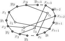
Figure 8.1: The graph $H$ with $\kappa_{3}(H)=2$

Later, Li and Mao [87] considered a generalization of the above problem. Let $s(n,k,\ell)$ and $t(n,k,\ell)$ denote the minimal number of edges of a graph $G$ of order $n$ with $\kappa_{k}(G)=\ell\ (1\leq\ell\leq n-\lceil\frac{k}{2}\rceil)$ and $\lambda_{k}(G)=\ell\ (1\leq\ell\leq n-\lceil\frac{k}{2}\rceil)$, respectively.

From Theorem 8.1, one can see that $s(n,3,2)=\lceil\frac{6}{5}n\rceil$ for all $n\geq 4$ but $n=9,10$. From Theorems 5.3 and 5.4, we know that

$$s(n,k,n-\lceil k/2\rceil)=t(n,k,n-\lceil k/2\rceil)=\left\{\begin{array}[]{ll}{n\choose 2},&for\ k\ even;\\ {n\choose 2}-\frac{k-1}{2},&for\ k\ odd.\end{array}\right.$$

From Theorems 5.5 and 5.6, we know that for $k$ even

$$s(n,k,n-\lceil k/2\rceil-1)={n\choose 2}-k+1$$

and

$$t(n,k,n-\lceil k/2\rceil-1)={n\choose 2}-\lfloor n/2\rfloor.$$

Li and Mao [87] investigated $t(n,3,\ell)$ and derived the following result.

Theorem 8.2

[87] Let $n$ be an integer with $n\geq 3$. Then

$(1)$ $t(n,3,n-2)={n\choose{2}}-1$;

$(2)$ $t(n,3,n-3)={n\choose{2}}-\lfloor\frac{n+3}{2}\rfloor$;

$(3)$ $t(n,3,1)=n-1$;

$(4)$ $t(n,3,\ell)\geq\big{\lceil}\frac{\ell(\ell+1)}{2\ell+1}n\big{\rceil}$ for $n\geq 11$ and $2\leq\ell\leq n-4$. Moreover, the bound is sharp.

The complete bipartite graph $G=K_{\ell,\ell+1}$ is a sharp example for the bound of Theorem 8.2.

In [77], Li focused on the following problem: Given any positive integer $n\geq 4$, is there a smallest integer $f(n)$ such that every graph of order $n$ and size $e(G)\geq f(n)$ has $\kappa_{3}(G)\geq 2$ ? She proved that every graph $G$ of order $n$ and size $e(G)=\frac{n^{2}}{2}-\frac{3n}{2}+3$ can be regarded as a graph obtained from $K_{n}$ by deleting $n-3$ edges. Since $\kappa_{3}(G)\geq 2$, $f(n)\leq\frac{n^{2}}{2}-\frac{3n}{2}+3$. On the other hand, let $G$ be a graph obtained from $K_{n-1}$ by adding a vertex $v$ and joining $v$ to one vertex of $K_{n-1}$. Clearly, the order is $n$ and the size is $\frac{n^{2}}{2}-\frac{3n}{2}+2$. But $\kappa_{3}(G)\leq\delta(G)=1$. So $f(n)>\frac{n^{2}}{2}-\frac{3n}{2}+2$. Thus, the following result is easily seen.

Proposition 8.3

[77] Given any positive integer $n\geq 4$, there exists a smallest integer $f(n)=\frac{n^{2}}{2}-\frac{3n}{2}+3$ such that every graph $G$ of order $n$ and size $e(G)\geq f(n)$ has $\kappa_{3}(G)\geq 2$.

Recall that a graph $G$ is minimal for $\kappa_{k}(G)=t$ if the generalized $k$-connectivity of $G$ is $t$ but the generalized $k$-connectivity of $G-e$ is less than $t$ for any edge $e$ of $G$. Though it is easy to find the sharp lower bound of $e(G)$, very little progress has been made on the sharp upper bound. So, Li phrased an open problem as follows.

Open Problem: Let $G$ be a graph of order $n$ and size $e(G)$ such that $G$ is minimal for $\kappa_{3}=2$. Find the sharp upper bounds $g(n)$ of $e(G)$.

She proved that $2n-4\leq g(n)\leq 3n-10$, but the exact value of $g(n)$ is still unknown.

8.2 Maximum generalized local connectivity

Recall that $\kappa(G)=\min\{\kappa_{G}(x,y)\,|\,x,y\in V(G),\ x\neq y\}$ is usually the connectivity of $G$. In contrast to this parameter, $\overline{\kappa}(G)=\max\{\kappa_{G}(x,y)\,|\,x,y\in V(G),\ x\neq y\}$, introduced by Bollobás, is called the maximum local connectivity of $G$. The problem of determining the smallest number of edges, $h(n;\overline{\kappa}\geq r)$, which guarantees that any graph with $n$ vertices and $h(n;\overline{\kappa}\geq r)$ edges will contain a pair of vertices joined by $r$ internally disjoint paths was posed by Erdös and Gallai; see [8] for details. Bollobás [15] considered the problem of determining the largest number of edges, $f(n;\overline{\kappa}\leq\ell)$, for graphs with $n$ vertices and local connectivity at most $\ell$, that is, $f(n;\overline{\kappa}\leq\ell)=\max\{e(G)\,|\,|V(G)|=n\ and\ \overline{\kappa}(G)\leq\ell\}$. One can see that $h_{1}(n;\overline{\kappa}\geq\ell+1)=f(n;\overline{\kappa}\leq\ell)+1$. Similarly, let $\lambda_{G}(x,y)$ denote the local edge-connectivity connecting $x$ and $y$ in $G$. Then $\lambda(G)=\min\{\lambda_{G}(x,y)\,|\,x,y\in V(G),\ x\neq y\}$ and $\overline{\lambda}(G)=\max\{\lambda_{G}(x,y)\,|\,x,y\in V(G),\ x\neq y\}$ are the edge-connectivity and maximum local edge-connectivity, respectively. So the edge version of the above problems can be given similarly. Set $g(n;\overline{\lambda}\leq\ell)=\max\{e(G)\,|\,|V(G)|=n\ and\ \overline{\lambda}(G)\leq\ell\}$. Let $h_{2}(n;\overline{\lambda}\geq r)$ denote the smallest number of edges which guarantees that any graph with $n$ vertices and $h_{2}(n;\overline{\kappa}\geq r)$ edges will contain a pair of vertices joined by $r$ edge-disjoint paths. Similarly, $h_{2}(n;\overline{\lambda}\geq\ell+1)=g(n;\overline{\lambda}\leq\ell)+1$. The problem of determining the precise value of the parameters $f(n;\overline{\kappa}\leq\ell)$, $g(n;\overline{\lambda}\leq\ell)$, $h_{1}(n;\overline{\kappa}\geq r)$, or $h_{2}(n;\overline{\kappa}\geq r)$ has obtained wide attention and many results have been worked out; see [15, 16, 17, 68, 69, 70, 94, 95, 123].

Similar to the classical maximum local connectivity, Li, Li and Mao [72] introduced the parameter $\overline{\kappa}_{k}(G)=\max\{\kappa(S)\,|\,S\subseteq V(G),\ |S|=k\}$, which is called the maximum generalized local connectivity of $G$. There they considered the problem of determining the largest number of edges, $f(n;\overline{\kappa}_{k}\leq\ell)$, for graphs with $n$ vertices and maximal generalized local connectivity at most $\ell$, that is, $f(n;\overline{\kappa}_{k}\leq\ell)=\max\{e(G)\,|\,|V(G)|=n\ and\ \overline{\kappa}_{k}(G)\leq\ell\}$. They also considered the smallest number of edges, $h_{1}(n;\overline{\kappa}_{k}\geq r)$, which guarantees that any graph with $n$ vertices and $h_{1}(n;\overline{\kappa}_{k}\geq r)$ edges will contain a set $S$ of $k$ vertices such that there are $r$ internally disjoint $S$-trees. It is easy to check that $h_{1}(n;\overline{\kappa}_{k}\geq\ell+1)=f(n;\overline{\kappa}_{k}\leq\ell)+1$ for $0\leq\ell\leq n-\lceil k/2\rceil-1$.

The edge version of these problems are also introduced and investigated by Li and Mao in [85]. Similarly, $g(n;\overline{\lambda}_{k}\leq\ell)=\max\{e(G)\,|\,|V(G)|=n\ and\ \overline{\lambda}_{k}(G)\leq\ell\}$, and $h_{2}(n;\overline{\lambda}_{k}\geq r)$ is the smallest number of edges, $h_{2}(n;\overline{\lambda}_{k}\geq r)$, which guarantees that any graph with $n$ vertices and $h_{2}(n;\overline{\lambda}_{k}\geq r)$ edges will contain a set $S$ of $k$ vertices such that there are $r$ edge-disjoint $S$-trees, and also similarly, $h_{2}(n;\overline{\lambda}_{k}\geq\ell+1)=g(n;\overline{\lambda}_{k}\leq\ell)+1$ for $0\leq\ell\leq n-\lceil k/2\rceil-1$.

In order to make the parameter $f(n;\overline{\lambda}_{k}\leq\ell)$ to be meaningful, we need to determine the range of $\ell$. In fact, with the help of the definitions of $\overline{\kappa}_{k}(G)$, $\kappa_{k}(G)$, $\overline{\lambda}_{k}(G)$, $\lambda_{k}(G)$ and Theorems 2.3 and 2.4, Li and Mao got the following observation, which implies that $1\leq\ell\leq n-\lceil k/2\rceil$.

Observation 8.4

[85] Let $k,n$ be two integers with $3\leq k\leq n$. Then for a connected graph $G$ of order $n$, $1\leq\overline{\kappa}_{k}(G)\leq\overline{\lambda}_{k}(G)\leq n-\lceil k/2\rceil$. Moreover, the upper and lower bounds are sharp.

Let us now introduce a graph class $\mathcal{G}_{n}^{*}$ by a few steps. For $r\geq 5$, $\mathcal{G}_{n}=\{H_{r}^{1},H_{r}^{2},H_{r}^{3},H_{r}^{4},\linebreak[2]H_{r}^{5},H_{r}^{6},H_{r}^{7}\}$ is a class of graphs of order $r$ (see Figure $8.2$ for details).

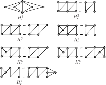
Figure 8.2: The graph class $\mathcal{G}_{n}$

Li, Li and Mao introduced a graph operation. Let $H$ be a connected graph, and $u$ a vertex of $H$. They defined the attaching operation at the vertex $u$ on $H$ as follows:

$\bullet$ identifying $u$ and a vertex of a $K_{4}$;

$\bullet$ $u$ is attached with only one $K_{4}$.

The vertex $u$ is called an attaching vertex.

Let $\mathcal{H}_{n}^{i}\ (1\leq i\leq 7)$ be the class of graphs, each of them is obtained from a graph $H_{r}^{i}$ by the attaching operation at some vertices of degree $2$ on $H_{r}^{i}$, where $3\leq r\leq n$ and $1\leq i\leq 7$ (note that $H_{n}^{i}\in\mathcal{H}_{n}^{i}$). $\mathcal{G}_{n}^{*}$ is another class of graphs that contains $\mathcal{G}_{n}$, given as follows: $\mathcal{G}_{3}^{*}=\{K_{3}\}$, $\mathcal{G}_{4}^{*}=\{K_{4}\}$, $\mathcal{G}_{5}^{*}=\{G_{1}\}\cup(\bigcup_{i=1}^{7}\mathcal{H}_{5}^{i})$, $\mathcal{G}_{6}^{*}=\{G_{3},G_{4}\}\cup(\bigcup_{i=1}^{7}\mathcal{H}_{6}^{i})$, $\mathcal{G}_{7}^{*}=\bigcup_{i=1}^{7}\mathcal{H}_{7}^{i}$, $\mathcal{G}_{8}^{*}=\{G_{2}\}\cup(\bigcup_{i=1}^{7}\mathcal{H}_{8}^{i})$, $\mathcal{G}_{n}^{*}=\bigcup_{i=1}^{7}\mathcal{H}_{n}^{i}$ for $n\geq 9$ (see Figure $8.3$ for details).

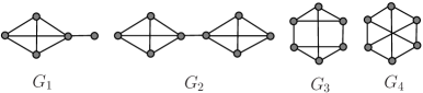
Figure 8.3: The graphs for Theorem 8.5

They obtained the following theorem.

Theorem 8.5

[72] Let $G$ be a connected graph of order $n$ such that $\overline{\kappa}_{3}(G)\leq 2$. Then

$$e(G)\leq\left\{\begin{array}[]{ll}2n-2,&if~{}n=4;\\ 2n-3,&if~{}n\geq 3,~{}n\neq 4.\end{array}\right.$$

with equality if and only if $G\in\mathcal{G}_{n}^{*}$.

By the definition of $f(n;\overline{\kappa}_{k}\leq\ell)$, the following corollary is immediate.

Corollary 8.6

[72]

$$f(n;\overline{\kappa}_{3}\leq 2)=\left\{\begin{array}[]{ll}2n-2&if~{}n=4;\\ 2n-3&if~{}n\geq 3,~{}n\neq 4.\end{array}\right.$$

For a general $\ell$, they constructed a graph class to give a lower bound of $f(n;\overline{\kappa}_{3}\leq\ell)$.

Example 8.2. Let $n,\ell$ be odd, and $G^{\prime}$ be a graph obtained from an $(\ell-3)$-regular graph of order $n-2$ by adding a maximum matching, and $G=G^{\prime}\vee K_{2}$. Then $\delta(G)=\ell-1$, $\overline{\kappa}_{3}(G)\leq\ell$ and $e(G)=\frac{\ell+2}{2}(n-2)+\frac{1}{2}$.

Otherwise, let $G^{\prime}$ be an $(\ell-2)$-regular graph of order $n-2$ and $G=G^{\prime}\vee K_{2}$. Then $\delta(G)=\ell$, $\overline{\kappa}_{3}(G)\leq\ell$ and $e(G)=\frac{\ell+2}{2}(n-2)+1$.

Therefore,

$$f(n;\overline{\kappa}_{3}\leq\ell)\geq\left\{\begin{array}[]{cc}\frac{\ell+2}{2}(n-2)+\frac{1}{2}&for~{}n,\ell~{}odd,\\ \frac{\ell+2}{2}(n-2)+1&~{}otherwise.\end{array}\right.$$

One can see that for $\ell=2$ this bound is the best possible ($f(n;\overline{\kappa}_{3}\leq 2)=2n-3$). Actually, the graph constructed for this bound is $K_{2}\vee(n-2)K_{1}$, which belongs to $\mathcal{G}_{n}^{*}$.

Li and Zhao [91] investigated the exact value of $f(n;\overline{\kappa}_{k}=1)$. They introduced the following operation and graph class: Let $H_{1}$ and $H_{2}$ be two connected graphs. We obtain a graph $H_{1}+H_{2}$ from $H_{1}$ and $H_{2}$ by joining an edge $uv$ between $H_{1}$ and $H_{2}$ where $u\in H_{1}$, $v\in H_{2}$. We call this operation the adding operation. $\{C_{3}\}^{i}+\{C_{4}\}^{j}+\{C_{5}\}^{k}+\{K_{1}\}^{l}$ is a class of connected graphs obtained from $i$ copies of $C_{3}$, $j$ copies of $C_{4}$, $k$ copies of $C_{5}$ and $\ell$ copies of $K_{1}$ by some adding operations such that $0\leq i\leq\lfloor\frac{n}{3}\rfloor$, $0\leq j\leq 2$, $0\leq k\leq 1$, $0\leq\ell\leq 2$ and $3i+4j+5k+\ell=n$. Note that these operations are taken in an arbitrary order.

The following graphs shown in Figure $8.4$ will be used later.

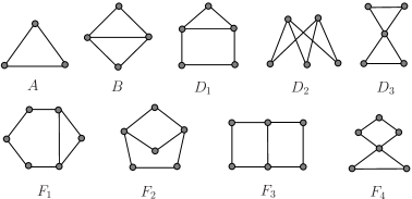
Figure 8.4: Graphs for $f(n;\overline{\kappa}_{k}=1)$.

At first, they studied the exact value of $f(n;\overline{\kappa}_{3}=1)$ and characterized the graphs attaining this value.

Theorem 8.7

[91] Let $n=3r+q\ (0\leq q\leq 2)$, and let $G$ be a connected graph of order $n$ such that $\overline{\kappa}_{3}(G)=1$. Then

$$e(G)\leq\frac{4n-3-q}{3}$$

with equality if and only if $G\in\mathcal{G}_{n}^{q}$.

The graph class $\mathcal{G}_{n}^{q}$ is defined as follows: Let $n=3r+q$, $0\leq q\leq 2$. If $q=0$, $\mathcal{G}_{n}^{0}=\{C_{3}\}^{r}$. If $q=1$, $\mathcal{G}_{n}^{1}=\{C_{3}\}^{r}+K_{1}$ or $\{C_{3}\}^{r-1}+C_{4}$. If $q=2$, $\mathcal{G}_{n}^{2}=\{C_{3}\}^{r}+\{K_{1}\}^{2}$ or $\{C_{3}\}^{r-1}+C_{4}+K_{1}$ or $\{C_{3}\}^{r-1}+C_{5}$ or $\{C_{3}\}^{r-2}+\{C_{4}\}^{2}$.

Next, they investigated the exact value of $f(n;\overline{\kappa}_{4}=1)$ and characterized the graphs attaining this value.

Theorem 8.8

[91] Let $n=4r+q$ where $0\leq q\leq 3$, and let $G$ be a connected graph of order $n$ such that $\overline{\kappa}_{4}(G)=1$. Then

$$e(G)\leq\left\{\begin{array}[]{cc}\frac{3n-2}{2}&if~{}q=0,\\ \frac{3n-3}{2}&if~{}q=1,\\ \frac{3n-4}{2}&if~{}q=2,\\ \frac{3n-3}{2}&if~{}q=3.\end{array}\right.$$

with equality if and only if $G\in\mathcal{H}_{n}^{q}$.

The graph class $\{A\}^{i_{0}}+\{B\}^{i_{1}}+\{D_{1}\}^{i_{2}}+\{D_{2}\}^{i_{3}}+\{D_{3}\}^{i_{4}}+\{F_{1}\}^{i_{5}}+\{F_{2}\}^{i_{6}}+\{F_{3}\}^{i_{7}}+\{F_{4}\}^{i_{8}}+\{K_{1}\}^{i_{9}}$ is composed of another connected graph class by some adding operations satisfying the following conditions:

$\bullet$ $0\leq i_{0}\leq 2$, $0\leq i_{1}\leq\lfloor\frac{n}{4}\rfloor$, $0\leq i_{2}+i_{3}+i_{4}\leq 2$, $0\leq i_{5}+i_{6}+i_{7}+i_{8}\leq 1$, $0\leq i_{9}\leq 2$;

$\bullet$ $D_{i}$ and $F_{j}$ are not simultaneously in a graph belonging to this graph class where $1\leq i\leq 3$, $1\leq j\leq 4$;

$\bullet$ $3i_{0}+4i_{1}+5(i_{2}+i_{3}+i_{4})+6(i_{5}+i_{6}+i_{7}+i_{8})+i_{9}=n$.

The graph class $\mathcal{H}_{n}^{q}$ is defined as follows: Let $n=4r+q$, $0\leq q\leq 3$. If $q=0$, $\mathcal{H}_{n}^{0}=\{B\}^{r}$; If $q=1$, $\mathcal{H}_{n}^{1}=\{B\}^{r}+K_{1}$ or $\{B\}^{r-1}+D_{i}\ (1\leq i\leq 3$); If $q=2$, $\mathcal{H}_{n}^{2}=\{B\}^{r}+\{K_{1}\}^{2}$ or $\{B\}^{r-1}+\{A\}^{2}$ or $\{B\}^{r-1}+D_{i}+K_{1}$ or $\{B\}^{r-2}+D_{i}+D_{j}\ (1\leq i,j\leq 3)$ or $\{B\}^{r-1}+F_{i}\ (1\leq i\leq 4)$; If $q=3$, $\mathcal{H}_{n}^{3}=\{B\}^{r}+A$.

For a graph $G$, we say that a path $P=u_{1}u_{2}\cdots u_{q}$ is an ear of G if $V(G)\cap V(P)=\{u_{1},u_{q}\}$. If $u_{1}\neq u_{q}$, $P$ is an open ear; otherwise $P$ is a closed ear. In their proofs of Theorems 8.7 and 8.8, they got necessary and sufficient conditions for $\overline{\kappa}_{k}(G)=1$ with $k=3,4$ by means of the number of ears of cycles. Naturally, one might think that this method can always be applied for $k=5$, i.e., every cycle in $G$ has at most two ears, but unfortunately they found a counterexample.

Example 8.3. Let $G$ be a graph which contains a cycle with three independent closed ears. Set $C=u_{1}u_{2}u_{3}$, $P_{1}=u_{1}v_{1}w_{1}u_{1}$, $P_{2}=u_{2}v_{2}w_{2}u_{2}$, and $P_{3}=u_{3}v_{3}w_{3}u_{3}$. Then, $\overline{\kappa}_{5}(G)=1$. In fact, let $S$ be the set of chosen five vertices. Obviously, for each $i$, if $v_{i}$ and $w_{i}$ are in $S$, then $\overline{\kappa}_{k}(S)=1$. So, only one vertex in $P_{i}\setminus u_{i}$ can be chosen. Suppose that $v_{1},v_{2},v_{3}$ have been chosen. By symmetry, $u_{1},u_{2}$ are chosen. It is easy to check that there is only one tree connecting $\{u_{1},u_{2},v_{1},v_{2},v_{3}\}$. The remaining case is that all $u_{1}$, $u_{2}$ and $u_{3}$ are chosen. Then, no matter which are the another two vertices, only one tree can be found.

For a general $k$ with $5\leq k\leq n-1$, they obtained the following lower bound of $f(n;\overline{\kappa}_{k}(G)=1)$ by constructing a graph class as follows: If $q=0$, let $G=\{K_{k-1}\}^{r}$, then $e(G)=r{k-1\choose 2}+r-1$. If $1\leq q\leq k$, let $G=\{K_{k-1}\}^{r}+K_{q}$, then $e(G)=r{k-1\choose 2}+{q\choose 2}+r$. So the following proposition is immediate.

Proposition 8.9

[91] For $n=r(k-1)+q\ (0\leq q\leq k-2)$,

$$f(n;\overline{\kappa}_{k}=1)\geq\left\{\begin{array}[]{ll}r{k-1\choose 2}+r-1,&\hbox{if~{}$q=0$;}\\ r{k-1\choose 2}+{q\choose 2}+r,&\hbox{if~{}$1\leq q\leq k-2$.}\end{array}\right.$$

Actually, Li and Zhao also got the exact value of $f(n;\overline{\kappa}_{k}=1)$ for $k=n$.

Theorem 8.10

[91] Let $G$ be a connected graph of order $n$ such that $\overline{\kappa}_{n}(G)=1$ where $n\geq 5$. Then

$$e(G)\leq{n-1\choose 2}+1$$

with equality if and only if $G\in\mathcal{K}_{n}$.

The graph class $\mathcal{K}_{n}$ is defined as follows: for $n=5$, $\mathcal{K}_{5}=\{G:|V(G)|=5,e(G)=7\}$; for $n\geq 6$, $\mathcal{K}_{n}=K_{n-1}+K_{1}$.

The following three corollaries are immediate from Theorems 8.7, 8.8 and 8.10.

Corollary 8.11

[91] For $n=3r+q\ (0\leq q\leq 2)$,

$$f(n;\overline{\kappa}_{3}=1)=\frac{4n-3-q}{3}$$

.

Corollary 8.12

[91] For $n=4r+q\ (0\leq q\leq 3)$,

$$f(n;\overline{\kappa}_{4}=1)=\left\{\begin{array}[]{cc}\frac{3n-2}{2}&if~{}q=0,\\ \frac{3n-3}{2}&if~{}q=1,\\ \frac{3n-4}{2}&if~{}q=2,\\ \frac{3n-3}{2}&if~{}q=3.\end{array}\right.$$

Corollary 8.13

[91] For $n\geq 5$, $f(n;\overline{\kappa}_{n}=1)={n-1\choose 2}+1$.

Later, Li and Mao continued to study the above problems. Note that for $k=n$ we have $1\leq\ell\leq\lfloor\frac{n}{2}\rfloor$ by Observation 8.4. With the help of Theorem 1.3 (due to Nash-Williams and Tutte), they determined the exact value of $f(n;\overline{\kappa}_{k}\leq\ell)$ for $k=n$.

Theorem 8.14

[85] Let $G$ be a connected graph of order $n\ (n\geq 6)$. If $\overline{\lambda}_{n}(G)\leq\ell\ (1\leq\ell\leq\lfloor\frac{n}{2}\rfloor)$, then

$$e(G)\leq\left\{\begin{array}[]{ll}{{n-1}\choose{2}}+\ell,&if~{}1\leq\ell\leq\lfloor\frac{n-4}{2}\rfloor;\\ {{n-1}\choose{2}}+n-2,&if~{}\ell=\lfloor\frac{n-2}{2}\rfloor~{}and~{}$n$~{}is~{}even;\\ {{n-1}\choose{2}}+\frac{n-3}{2},&if~{}\ell=\lfloor\frac{n-2}{2}\rfloor~{}and~{}$n$~{}is~{}odd;\\ {{n}\choose{2}},&if~{}\ell=\lfloor\frac{n}{2}\rfloor.\end{array}\right.$$

with equality if and only if $G\in\mathcal{G}_{n}$ for $1\leq\ell\leq\lfloor\frac{n-4}{2}\rfloor$ where $\mathcal{G}_{n}$ is a graph class obtained from a complete graph $K_{n-1}$ by adding a vertex $v$ and joining $v$ to $\ell$ vertices of $K_{n-1}$; $G=K_{n}\setminus e$ where $e\in E(K_{n})$ for $\ell=\lfloor\frac{n-2}{2}\rfloor$ and $n$ even; $G=K_{n}\setminus M$ where $M\subseteq E(K_{n})$ and $|M|=\frac{n+1}{2}$ for $\ell=\lfloor\frac{n-2}{2}\rfloor$ and $n$ odd; $G=K_{n}$ for $\ell=\lfloor\frac{n}{2}\rfloor$.

From the definition of $f(n;\overline{\kappa}_{n}\leq\ell)$ and $g(n;\overline{\lambda}_{n}\leq\ell)$, the following corollary is immediate.

Corollary 8.15

[85] For $1\leq\ell\leq\lfloor\frac{n}{2}\rfloor$ and $n\geq 6$,

$$f(n;\overline{\kappa}_{n}\leq\ell)=g(n;\overline{\lambda}_{n}\leq\ell)=\left\{\begin{array}[]{ll}{{n-1}\choose{2}}+\ell,&if~{}1\leq\ell\leq\lfloor\frac{n-4}{2}\rfloor~{}or~{}\ell=\lfloor\frac{n-2}{2}\rfloor~{}and~{}$n$~{}is~{}odd;\\ {{n-1}\choose{2}}+2\ell,&if~{}\ell=\lfloor\frac{n-2}{2}\rfloor~{}and~{}$n$~{}is~{}even;\\ {{n}\choose{2}},&if~{}\ell=\lfloor\frac{n}{2}\rfloor.\end{array}\right.$$

For $k=n-1$, $1\leq\ell\leq\lfloor\frac{n+1}{2}\rfloor$ by Observation 8.4. In order to determine the exact value of $f(n;\overline{\kappa}_{n-1}\leq\ell)$ for a general $\ell\ (1\leq\ell\leq\lfloor\frac{n+1}{2}\rfloor)$, Li and Mao first focused on the cases $\ell=\lfloor\frac{n+1}{2}\rfloor$ and $\lfloor\frac{n-1}{2}\rfloor$. This is also because by characterizing the graphs with $\overline{\kappa}_{n-1}(G)=\lfloor\frac{n+1}{2}\rfloor$ and $\lfloor\frac{n-1}{2}\rfloor$, the difficult case $\ell=\lfloor\frac{n-3}{2}\rfloor$ can be dealt with. Next, they considered the case $1\leq\ell\leq\lfloor\frac{n-5}{2}\rfloor$ and summarized the results for a general $\ell$.

Theorem 8.16

[85] Let $G$ be a connected graph of order $n\ (n\geq 12)$. If $\overline{\kappa}_{n-1}(G)\leq\ell\ (1\leq\ell\leq\lfloor\frac{n+1}{2}\rfloor)$, then

$$e(G)\leq\left\{\begin{array}[]{ll}{{n-2}\choose{2}}+2\ell,&if~{}1\leq\ell\leq\lfloor\frac{n-5}{2}\rfloor;\\ {{n-2}\choose{2}}+n-2,&if~{}\ell=\lfloor\frac{n-3}{2}\rfloor~{}and~{}$n$~{}is~{}odd;\\ {{n-2}\choose{2}}+n-4,&if~{}\ell=\lfloor\frac{n-3}{2}\rfloor~{}and~{}$n$~{}is~{}even;\\ {{n-1}\choose{2}}+n-2,&if~{}\ell=\lfloor\frac{n-1}{2}\rfloor~{}and~{}$n$~{}is~{}odd;\\ {{n-1}\choose{2}}+\frac{n-2}{2},&if~{}\ell=\lfloor\frac{n-1}{2}\rfloor~{}and~{}$n$~{}is~{}even;\\ {{n}\choose{2}},&if~{}\ell=\lfloor\frac{n+1}{2}\rfloor.\end{array}\right.$$

with equality if and only if $G\in\mathcal{H}_{n}$ for $1\leq\ell\leq\lfloor\frac{n-5}{2}\rfloor$ where $\mathcal{H}_{n}$ is a graph class obtained from the complete graph of order $n-2$ by adding two nonadjacent vertices and joining each of them to any $\ell$ vertices of $K_{n-2}$; $G=K_{n}\setminus M$ where $|M|=n-1$ for $\ell=\lfloor\frac{n-3}{2}\rfloor$ and $n$ odd; $G\in\mathcal{H}_{n}$ for $\ell=\lfloor\frac{n-3}{2}\rfloor$ and $n$ even; $G=K_{n}\setminus e$ where $e\in E(K_{n})$ for $\ell=\lfloor\frac{n-1}{2}\rfloor$ and $n$ odd; $G=K_{n}\setminus M$ where $|M|=\frac{n}{2}$ for $\ell=\lfloor\frac{n-1}{2}\rfloor$ and $n$ even; $G=K_{n}$ for $\ell=\lfloor\frac{n+1}{2}\rfloor$.

The following corollary is immediate from Theorem 8.16.

Corollary 8.17

[85] For $1\leq\ell\leq\lfloor\frac{n+1}{2}\rfloor$ and $n\geq 12$,

$$f(n;\overline{\kappa}_{n-1}\leq\ell)=\left\{\begin{array}[]{ll}{{n-2}\choose{2}}+2\ell,&if~{}1\leq\ell\leq\lfloor\frac{n-5}{2}\rfloor,~{}or~{}\ell=\lfloor\frac{n-3}{2}\rfloor~{}and~{}$n$~{}is~{}even;\\ {{n-2}\choose{2}}+2\ell+1,&if~{}\ell=\lfloor\frac{n-3}{2}\rfloor~{}and~{}$n$~{}is~{}odd;\\ {{n-1}\choose{2}}+\ell,&if~{}\ell=\lfloor\frac{n-1}{2}\rfloor~{}and~{}$n$~{}is~{}even;\\ {{n-1}\choose{2}}+2\ell-1,&if~{}\ell=\lfloor\frac{n-1}{2}\rfloor~{}and~{}$n$~{}is~{}odd;\\ {{n}\choose{2}},&if~{}\ell=\lfloor\frac{n+1}{2}\rfloor.\end{array}\right.$$

Applying Theorem 8.16 and the relation between $\overline{\kappa}_{k}$ and $\overline{\lambda}_{k}$, they investigated the edge case and derived the following result.

Theorem 8.18

[85] Let $G$ be a connected graph of order $n\ (n\geq 12)$. If $\overline{\lambda}_{n-1}(G)\leq\ell\ (1\leq\ell\leq\lfloor\frac{n+1}{2}\rfloor)$, then

$$e(G)\leq\left\{\begin{array}[]{ll}{{n-2}\choose{2}}+2\ell,&if~{}1\leq\ell\leq\lfloor\frac{n-5}{2}\rfloor;\\ {{n-2}\choose{2}}+n-2,&if~{}\ell=\lfloor\frac{n-3}{2}\rfloor~{}and~{}$n$~{}is~{}odd;\\ {{n-2}\choose{2}}+n-4,&if~{}\ell=\lfloor\frac{n-3}{2}\rfloor~{}and~{}$n$~{}is~{}even;\\ {{n-1}\choose{2}}+n-2,&if~{}\ell=\lfloor\frac{n-1}{2}\rfloor~{}and~{}$n$~{}is~{}odd;\\ {{n-1}\choose{2}}+\frac{n-2}{2},&if~{}\ell=\lfloor\frac{n-1}{2}\rfloor~{}and~{}$n$~{}is~{}even;\\ {{n}\choose{2}},&if~{}\ell=\lfloor\frac{n+1}{2}\rfloor.\end{array}\right.$$

with equality if and only if $G\in\mathcal{H}_{n}$ for $1\leq\ell\leq\lfloor\frac{n-5}{2}\rfloor$ where $\mathcal{H}_{n}$ is a graph class obtained from the complete graph of order $n-2$ by adding two nonadjacent vertices and joining each of them to any $\ell$ vertices of $K_{n-2}$; $G=K_{n}\setminus M$ where $|M|=n-1$ for $\ell=\lfloor\frac{n-3}{2}\rfloor$ and $n$ odd; $G\in\mathcal{H}_{n}$ for $\ell=\lfloor\frac{n-3}{2}\rfloor$ and $n$ even; $G=K_{n}\setminus e$ where $e\in E(K_{n})$ for $\ell=\lfloor\frac{n-1}{2}\rfloor$ and $n$ odd; $G=K_{n}\setminus M$ where $|M|=\frac{n}{2}$ for $\ell=\lfloor\frac{n-1}{2}\rfloor$ and $n$ even; $G=K_{n}$ for $\ell=\lfloor\frac{n+1}{2}\rfloor$.

Corollary 8.19

[85] For $1\leq\ell\leq\lfloor\frac{n+1}{2}\rfloor$ and $n\geq 12$,

$$g(n;\overline{\lambda}_{n-1}\leq\ell)=\left\{\begin{array}[]{ll}{{n-2}\choose{2}}+2\ell,&if~{}1\leq\ell\leq\lfloor\frac{n-5}{2}\rfloor,~{}or~{}\ell=\lfloor\frac{n-3}{2}\rfloor~{}and~{}$n$~{}is~{}even;\\ {{n-2}\choose{2}}+2\ell+1,&if~{}\ell=\lfloor\frac{n-3}{2}\rfloor~{}and~{}$n$~{}is~{}odd;\\ {{n-1}\choose{2}}+\ell,&if~{}\ell=\lfloor\frac{n-1}{2}\rfloor~{}and~{}$n$~{}is~{}even;\\ {{n-1}\choose{2}}+2\ell-1,&if~{}\ell=\lfloor\frac{n-1}{2}\rfloor~{}and~{}$n$~{}is~{}odd;\\ {{n}\choose{2}},&if~{}\ell=\lfloor\frac{n+1}{2}\rfloor.\end{array}\right.$$

Remark 8.20

It is not easy to determine the exact value of $f(n;\overline{\kappa}_{k}\leq\ell)$ and $g(n;\overline{\lambda}_{k}\leq\ell)$ for a general $k$. So they hoped to give a sharp lower bound of them. They construct a graph $G$ of order $n$ as follows: Choose a complete graph $K_{k-1}\ (1\leq\ell\leq\lfloor\frac{k-1}{2}\rfloor)$. For the remaining $n-k+1$ vertices, join each of them to any $\ell$ vertices of $K_{k-1}$. Clearly, $\overline{\kappa}_{n-1}(G)\leq\overline{\lambda}_{n-1}(G)\leq\ell$ and $e(G)={{k-1}\choose{2}}+(n-k+1)\ell$. So $f(n;\overline{\kappa}_{k}\leq\ell)\geq{{k-1}\choose{2}}+(n-k+1)\ell$ and $g(n;\overline{\lambda}_{k}\leq\ell)\geq{{k-1}\choose{2}}+(n-k+1)\ell$. From Theorems 8.16 and 8.18, one knows that these two bounds are sharp for $k=n,n-1$.

9 For random graphs

In this section, we survey the results for random graphs. The two most frequently occurring probability models of random graphs are $G(n,M)$ and $G(n,p)$. The first consists of all graphs with $n$ vertices having $M$ edges, in which the graphs have the same probability. The model $G(n,p)$ consists of all graphs with $n$ vertices in which the edges are chosen independently and with probability $p$. Given sequences $a_{n}$ and $b_{n}$ of real numbers (possibly taking negative values), we write $a_{n}=O(b_{n})$ if there is a constant $C>0$ such that $|a_{n}|\leq C|b_{n}|$ for all $n$; write $a_{n}=o(b_{n})$ if $lim_{n\rightarrow\infty}a_{n}/b_{n}=0$. Write $a_{n}=\Omega(b_{n})$ if $a_{n}\geq 0$ and $b_{n}=O(a_{n})$; $a_{n}=\omega(b_{n})$ if $a_{n}\geq 0$ and $b_{n}=o(a_{n})$; $a_{n}=\Theta(b_{n})$ if $a_{n}\geq 0$, $a_{n}=\Omega(b_{n})$ and $a_{n}=\Theta(b_{n})$. We say that an event $\mathcal{A}$ happens almost surely if the probability that it happens approaches $1$ as $n\rightarrow\infty$, i.e., $Pr[\mathcal{A}]=1-o_{n}(1)$. Sometimes, we say a.s. for short. We will always assume that $n$ is the variable that tends to infinity. Given a sequence of events $(E_{n})_{n\in N}$, we say that $E_{n}$ happens asymptotically almost surely $(a.a.s.)$ if $Pr(E_{n})\rightarrow 1$ as $n\rightarrow\infty$.

For a graph property $P$, a function $p(n)$ is called a threshold function of $P$ if:

• for every $r(n)=O(p(n))$, $G(n,r(n))$ almost surely satisfies $P$ ; and

• for every $r^{\prime}(n)=o(p(n))$, $G(n,r^{\prime}(n))$ almost surely does not satisfy $P$.

Furthermore, $p(n)$ is called a sharp threshold function of $P$ if there exist two positive constants $c$ and $C$ such that:

• for every $r(n)\geq C\cdot p(n)$, $G(n,r(n))$ almost surely satisfies $P$ ; and

• for every $r^{\prime}(n)\leq c\cdot p(n)$, $G(n,r^{\prime}(n))$ almost surely does not satisfy $P$.

9.1 Results for $k=n$

The spanning tree packing problem has long been one of the main motives in Graph Theory. Frieze and Luczak [41] firstly considered the maximum number of edge-disjoint spanning trees contained in the random graph $G_{k\text{-out}}$, and studied the random graph $G_{k}=G_{k\text{-out}}$. This random graph has vertex set $V=\{1,2,\cdots,n\}$. Each $v\in V_{n}$ independently chooses a set $out(v)$ of distinct vertices as neighbours, where each $k$-subset of $V_{n}-\{v\}$ is equally likely to be chosen. This produces a random $k$ out-regular diagraph $D_{k}$, which has been selected uniformly from $(\frac{n-1}{k})^{n}$ distinct possibilities, where $G_{k}$ is obtained by ignoring orientation but without coalescing edges; see [37, 40] for properties of this model. They obtained that for a fixed integer $k\geq 2$ the random graph $G_{k\text{-out}}$ almost surely has $k$ edge-disjoint spanning trees.

Moreover, Palmer and Spencer [110] proved that in almost every random graph process, the hitting time for having $k$ edge-disjoint spanning trees equals the hitting time for having minimum degree $k$, for any fixed positive integer $k$. In other words, considering the random graph $G(n,p)$, for any fixed positive integer $k$, if $p(n)\leq\frac{\log n+k\log\log n-\omega(1)}{n}$ (which is the maximal $p$ for which $\delta(G(n,p))\leq k$ a.s.), the probability that the spanning tree packing number equals the minimum degree approaches to $1$ as $n\rightarrow\infty$. On the other hand, in Catlin’s paper [21] it was found that if the edge probability was rather large, then almost surely the random graph $G(n,p)$ has $\lambda_{n}(G)=\lfloor|E(G)|/(n-1)\rfloor$, which is less than the minimum degree of $G$. We refer papers [21] and [109] to the reader for more details.

A natural question is whether there exists a largest $p(n)$ such that for every $r^{\prime}(n)\leq p(n)$, almost surely the random graph $G(n,p)$ satisfies that the spanning tree packing number equals the minimum degree.

In [27], Chen, Li and Lian partly answered this question by establishing the following two theorems for multigraphs. The first theorem establishes a lower bound of $q(n)$ with $q(n)\geq(1.1\log n)/n$. Note that this bound for $p$ will allow the minimum degree to be a function of $n$, and in this sense they improved the result of Palmer and Spencer.

Theorem 9.1

[27] For any $p$ such that $(\log n+\omega(1))/n\leq p\leq(1.1\log n)/n$, almost surely the random graph $G\sim G(n,p)$ satisfies that the spanning tree packing number is equal to the minimum degree, i.e.

$$\lim_{n\rightarrow\infty}\mathbf{Pr}(\lambda_{n}(G)=\delta(G))=1.$$

The second theorem gives an upper bound of $q(n)$ with $q(n)\leq(51\log n)/n$.

Theorem 9.2

[27] For any $p$ such that $p\geq(51\log n)/n$, almost surely the random graph $G\sim G(n,p)$ satisfies that the spanning tree packing number is less than the minimum degree, i.e.,

$$\lim_{n\rightarrow\infty}\mathbf{Pr}(\lambda_{n}(G)<\delta(G))=1.$$

Remark 9.3

From Theorems 9.1 and 9.2, one can see that $\log n/n$ is a sharp threshold function for the graph property that the spanning tree packing number is equal to the minimum degree.

Later, Gao, Pérez-Gimsénez and Sato strengthened the previous results. In order to introduce their work, we first need more notations and concepts. Let $\bar{d}(G)=2m(G)/(|V(G)|-1)$. Note that $\bar{d}(G)$ differs from the average degree of $G$ by a small factor of $|V(G)|/(|V(G)|-1)$. In particular, in their paper, all constants involved in these notations do not depend on $p$ under discussion. For instance, if we have $a_{n}=\Omega(b_{n})$, where $b_{n}$ may be an expression involving $p=p(n)$, then it means that there are constants $C>0$ and $n_{0}$ (both independent with $p$), such that $a_{n}\geq C|b_{n}|$ uniformly for all $n\geq n_{0}$ and for all $p$ in the range under discussion. For any graph $G$, let $T(G)$ and $A(G)$ denote the maximum number of edge-disjoint spanning trees in $G$ (possibly $0$ if G is disconnected) and the minimum number of subforests of G which cover the whole edge set of $G$, respectively. This number $A(G)$ is known as the arboricity of $G$.

They proved that for all $p\in[0,1]$, the STP number is $a.a.s.$ the minimum between $\delta$ and $m/(n-1)$, where $\delta$ and $m$ respectively denote the minimum degree and the number of edges of $G(n,p)$.

Theorem 9.4

[42] For every $p=p(n)\in[0,1]$, we have that $a.a.s.$

$$T(G(n,p))=\min\left\{\delta(G(n,p)),\Big{\lfloor}\frac{\bar{d}(G(n,p))}{2}\Big{\rfloor}\right\}.$$

Note that the quantities $\delta$ and $m/(n-1)$ above correspond to the two trivial upper bounds observed earlier for arbitrary graphs, so this implies that we can $a.a.s.$ find a best-possible number of edge-disjoint spanning trees in $G(n,p)$. Their argument uses several properties of $G(n,p)$ in order to bound the number of crossing edges between subsets of vertices with certain restrictions, and then applies the characterization of the STP number by Tutte and Nash-Williams stated in Theorem 1.3. Moreover, they determined the ranges of $p$ for which the STP number takes each of these two values: $\delta$ and $m/(n-1)$. In spite of the fact that the property $\{\delta\leq m/(n-1)\}$ is not necessarily monotonic with respect to $p$, they showed that it has a sharp threshold at $p\sim\beta\log n/n$, where $\beta\approx 6.51778$ is a constant defined in the following theorem.

Theorem 9.5

[42] Let $\beta=2/\log(e/2)\approx 6.51778$. Then

$(1)$ if $p=\frac{\beta(\log n-\log\log n/2-\omega(1))}{n-1}$, then $a.a.s$ $\delta(G(n,p))\leq\big{\lfloor}\frac{\bar{d}(G(n,p))}{2}\big{\rfloor}$ and so $T(G(n,p))=\delta(G(n,p))$;

$(2)$ if $p=\frac{\beta(\log n-\log\log n/2+\omega(1))}{n-1}$, then $a.a.s$ $\delta(G(n,p))>\big{\lfloor}\frac{\bar{d}(G(n,p))}{2}\big{\rfloor}$ and so $T(G(n,p))=\delta(G(n,p))$.

Below this threshold, the STP number of $G(n,p)$ is $a.a.s.$ equal to $\delta$; and above the threshold it is $a.a.s.$ $m/(n-1)$. In particular, this settles the question raised by Chen, Li and Lian [27].

They further considered the random graph process $G_{0},G_{1},\cdots,G_{{n}\choose{2}}$ defined as follows: for each $m=0,\cdots,{{n}\choose{2}}$, $G_{m}$ is a graph with vertex set $[n]$; the graph $G_{0}$ has no edges; and, for each $1\leq m\leq{{n}\choose{2}}$, the graph $G_{m}$ is obtained by adding one new edge to $G_{m-1}$ chosen uniformly at random among the edges not present in $G_{m-1}$. Equivalently, we can choose uniformly at random a permutation $(e_{1},\cdots,e_{{{n}\choose{2}}})$ of the edges of the complete graph with vertex set $[n]$, and define each $G_{m}$ to be the graph on vertex set $[n]$ and edges $e_{1},\cdots,e_{m}$.

They also included a stronger version of these results in the context of the random graph process in which $p$ gradually grows from $0$ to $1$ (or, similarly, the edges are added one by one). This provides a full characterization of the STP number that holds $a.a.s.$ simultaneously during the whole random graph process.

Theorem 9.6

[42] Let $\beta=2/\log(e/2)\approx 6.51778$. The following holds in the random graph process $G_{0},G_{1},\cdots,G_{{n}\choose{2}}$.

$(1)$ $a.a.s$ $T(G_{m})=\min\{\delta(G_{m}),\lfloor m/(n-1)\rfloor\}$ for every $0\leq m\leq{{n}\choose{2}}$.

$(2)$ Moreover, for any constant $\epsilon>0$, $a.a.s$

$\bullet$ $\delta(G_{m})\leq\lfloor m/(n-1)\rfloor$ for every $0\leq m\leq\frac{(1-\epsilon)\beta}{2}n\log n$, and

$\bullet$ $\delta(G_{m})>\lfloor m/(n-1)\rfloor$ for every $\frac{(1-\epsilon)\beta}{2}n\log n\leq m\leq{{n}\choose{2}}$.

The argument combines a more accurate version of the same ideas used in the analysis of the STP number of $G(n,p)$ together with multiple couplings of $G(n,p)$ at different values of $p$. In addition, the article contains several results about the arboricity of $G(n,p)$. As an almost direct application of their result on the STP number, for $p$ above the threshold $\beta logn/n$, they determined the arboricity of $G(n,p)$ to be $a.a.s.$ equal to $m/(n-1)$. This significantly extends the range of $p$ in the result by Catlin, Chen and Palmer [21]. They further proved that for all other values of $p$, the arboricity of $G(n,p)$ is concentrated on at most two values.

Theorem 9.7

[42] Let $\beta=2/\log(e/2)\approx 6.51778$.

$(1)$ For all $p=\frac{\beta(\log n-\log\log n/2-\omega(1))}{n-1}$, $a.a.s$. $A(G(n,p))=\big{\lceil}\frac{\bar{d}(G(n,p))}{2}\big{\rceil}$; for all $p=\omega(1/n)$, $a.a.s$ $A(G(n,p))\in\left\{\big{\lceil}\frac{\bar{d}(G(n,p))}{2}\big{\rceil},\big{\lceil}\frac{\bar{d}(G(n,p))}{2}\big{\rceil}+1\right\}$;

$(2)$ For all $p=\Theta(1/n)$, $a.a.s$ $A(G(n,p))=(1+\Theta(1))pn/2$. Moreover, there exists a $k>0$ (depending on $p$), such that $a.a.s.$ $A(G(n,p))\in\{k,k+1\}$.

$(3)$ If $p=o(1/n)$, then $a.a.s.$ $A(G(n,p))\leq 1$.

In order to prove this for the case $pn\rightarrow\infty$, they added $o(n)$ edges to $G(n,p)$ in a convenient way that guarantees a full decomposition of the resulting graph into edge-disjoint spanning trees. This construction builds upon some of the ideas previously used to study the STP number. The case $pn=O(1)$ uses different proof techniques which rely on the structure of the $k$-core of $G(n,p)$ together with the Nash-Williams characterization of arboricity stated in Theorem 1.4.

Finally, some of the aforementioned results on the arboricity are also given below in the more precise context of the random graph process, similarly as they did for the STP number.

Theorem 9.8

[42] Let $\beta=2/\log(e/2)\approx 6.51778$. The following holds in the random graph process $G_{0},G_{1},\cdots,G_{{n}\choose{2}}$.

$(1)$ Let $m_{0}$ be any function of n such that $m_{0}/n\rightarrow\infty$ and let $\epsilon>0$ be any constant. Then, $a.a.s.$ simultaneously for all $m\geq m_{0}$ such that $\delta(G_{m})\leq\bar{d}(G_{m})/2$,

$$\Big{\lceil}\frac{m+\phi_{1}}{n-1}\Big{\rceil}\leq A(G_{m})\leq\Big{\lceil}\frac{m+\phi_{2}}{n-1}\Big{\rceil},$$

where $\phi_{1}=n/\exp(\frac{(1+\epsilon)}{\beta}\frac{2m}{n})=o(n)$ and $\phi_{1}=n/\exp(\frac{1-\epsilon}{\beta}\frac{2m}{n})=o(n)$. In particular, $a.a.s.$ $A(G_{m})\in\{\lceil\frac{m}{n-1}\rceil,\lceil\frac{m}{n-1}\rceil+1\}$ for all $m$ in that range.

$(2)$ Moreover, a.a.s. simultaneously for every m such that $\delta(G_{m})\geq\bar{d}(G_{m})/2$ we have

$$A(G_{m})\leq\lfloor m/(n-1)\rfloor.$$

Corollary 9.9

[42] Let $m_{A=i}$ denote the minimum $m$ such that $A(G_{m})$ becomes $i$ in the random graph process $G_{0},G_{1},\cdots,G_{{n}\choose{2}}$. Let $i_{0}$ be any function of $n$ such that $i_{0}\rightarrow\infty$ and $\epsilon>0$ be a constant. Then $a.a.s.$

$(1)$ for every $i_{0}\leq i\leq(1-\epsilon)\beta\log n/2$,

$$(i-1)(n-1)-\phi_{2}<m_{A=i}<(i-1)(n-1)-\phi_{1},$$

where $\phi_{1}=n/\exp(\frac{2(1+\epsilon)}{\beta}i)=o(n)$ and $\phi_{2}=n/\exp(\frac{2(1-\epsilon)}{\beta})=o(n)$; and

$(2)$ for every $(1+\epsilon)\beta\log n/2\leq i\leq n/2$,

$$m_{A=i}=(i-1)(n-1)+1$$

9.2 Results for $k=3$

As well-known, for the vertex connectivity, Bollobás and Thomason [19] gave the following result.

Theorem 9.10

[19] If $\ell\in\mathbb{N}$ and $y\in\mathbb{R}$ are fixed, and $M=\frac{n}{2}(\log n+\ell\log\log n+y+o(1))\in\mathbb{N}$, then

$$\Pr\left[{\kappa\left({G\left({n,M}\right)}\right)=\ell}\right]\to 1-{e^{-{e^{-y/\ell!}}}}$$

and

$$\Pr\left[{\kappa\left({G\left({n,M}\right)}\right)=\ell+1}\right]\to{e^{-{e^{-y/\ell!}}}}.$$

Gu, Li and Shi [48] focused their attention on the generalized $3$-connectivity of random graphs for simple graphs. They got the following theorem, which could be seen as a generalization of Theorem 9.10. At first, they proved that there exists a constant $c$ such that if $p^{\prime}<c\frac{{\log n+(\ell+1)\log\log n-\log\log\log n}}{n}$ then $\kappa_{3}(G(n,p))<\ell$ almost surely holds. Then, they showed that for any three vertices in $G(n,p)$, where $p=\frac{{\log n+(\ell+1)\log\log n-\log\log\log n}}{n}$, there almost surely exist three trees of some typical depths rooted at these three vertices, respectively. Combining some branches of these trees, $\ell$ internally disjoint trees connecting any three vertices can be constructed, which implies that $\kappa_{3}(G(n,p))\geq\ell$. Hence, they derived the following result.

Theorem 9.11

[48] Let $\ell\geq 1$ be a fixed integer. Then $p=\frac{{\log n+(\ell+1)\log\log n-\log\log\log n}}{n}$ is a sharp threshold function for the property $\kappa_{3}(G(n,p))\geq\ell$.

10 An application problem

For a network, we usually want to search for a minimum network such that some local parts have the connectivity we want and the other parts only need to be connected.

Li, Li and Mao [73] noticed an interesting problem: What is the smallest number of edges $f(n,k,\ell)$ for a connected graph $G$ of order $n$ that contains $\ell$ edge-disjoint $S$-Steiner trees for given $k$ vertices of $G$. They determined the exact value of the parameter $f(n,k,\ell)$ and characterized all the graphs attaining this value.

This problem has its strong application backgrounds. Suppose that $G$ is a secure information-gathering network. We denote by $S$ the set of core departments and each department wants to exchange important information with others. So we need some Steiner trees to connect them. But for a vertex not belonging to a Steiner tree, we let it be an agent. Usually an agent only needs to connect to its superior leader. So the global network should be connected.

A graph $G$ is called a $(k,\ell)$-minimum connected graph if $|V(G)|=n$, $e(G)=f(n,k,\ell)$ and there exist $\ell$ edge-disjoint $S$-trees for some $S\subseteq V(G)$ with $|S|=k$.

They obtained the exact value of $f(n,k,\ell)$.

Theorem 10.1

[73] For $3\leq k\leq n$, $f(n,k,\ell)=(k-1)\ell+n-k$.

Motivated by characterizing the $(k,\ell)$-minimum connected graphs, they first introduced the notion of an initial graph and three graph operations.

The initial graph. Let $k$ and $\ell$ be two integers, and $K_{1,k-1}$ be a star. Assume that $u_{1}$ is the center of the star $K_{1,k-1}$, and $u_{2},u_{3},\ldots,u_{k-1}$ are the leaves of the star. A $(k,\ell)$-initial graph is a graph obtained from the star $K_{1,k-1}$ by replacing each edge of $K_{1,k-1}$ by $\ell$ multiple edges. Clearly, the graph $G$ contains $\ell$ edge-disjoint spanning trees $T_{1},T_{2},\cdots,T_{\ell}$ such that each $T_{i}$ is a star $K_{1,k-1}$, that is, $u_{1}u_{2}\cup u_{1}u_{3}\cup\cup u_{1}u_{k-1}$. The edge-disjoint spanning trees $T_{1},T_{2},\cdots,T_{\ell}$ are called $(k,\ell)$-initial trees. Note that $G=\bigcup_{i=1}^{\ell}T_{i}$ and $G$ have $k$ vertices and $(k-1)\ell$ edges.

Operation I. For a tree $T_{i}$, we add an edge $e$ to $T_{i}$ such that $e\not\in E(T_{i})$ and $e$ joins two vertices of $T_{i}$. Thus $T_{i}+e$ contains a unique cycle, say $C$. Pick up an edge $e^{\prime}\in E(C)\ (e^{\prime}\neq e)$, then we obtain a new tree $T^{\prime}_{i}$ by deleting $e^{\prime}$ from $T_{i}+e$. Set $T_{i}:=T_{i}^{\prime}$ and $G:=\bigcup_{i=1}^{\ell}T_{i}$.

Operation II. For a tree $T_{i}$, pick up a vertex $v\in V(T_{i})$. Let $N=N_{T_{i}}(v)$. Divide $N$ into three subsets $N_{1},N_{2}$ and $N_{3}$ such that $N=N_{1}\cup N_{2}\cup N_{3}$ and $N_{3}=\{u\}$ (Note that $N_{1}$ and $N_{2}$ could be empty sets). Replace the vertex $v$ by two vertices $v^{\prime}$ and $v^{\prime\prime}$, and join $v^{\prime}$ to each vertex of $N_{1}$, $v^{\prime\prime}$ to each vertex of $N_{2}$, and $u$ to $v^{\prime}$ and $v^{\prime\prime}$. See Figure $10.1$ for details. If $v\in S$, then set $v:=v^{\prime}$; otherwise, we do nothing. Denote the new tree by $T_{i}^{\prime}$. Set $T_{i}:=T_{i}^{\prime}$ and $G:=\bigcup_{i=1}^{\ell}T_{i}$.

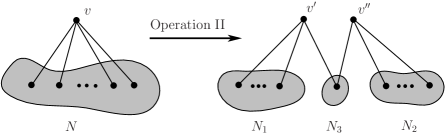
Figure 10.1: Operation II

Operation III. For a tree $T_{i}$, pick up a vertex $v\in V(T_{i})$. Let $N=N_{T_{i}}(v)$. Divide $N$ into two subsets $N_{1}$ and $N_{2}$ such that $N=N_{1}\cup N_{2}$ (Note that $N_{1}$ and $N_{2}$ could be empty sets). We replace vertex $v$ by two new vertices $v^{\prime}$ and $v^{\prime\prime}$, and join $v^{\prime}$ to each vertex of $N_{1}$, $v^{\prime\prime}$ to each vertex of $N_{2}$, and join $v^{\prime}$ to $v^{\prime\prime}$. See Figure $10.2$ for details. If $v\in S$, then set $v:=v^{\prime}$; otherwise, we do nothing. Set $T_{i}:=T_{i}^{\prime}$ and $G:=\bigcup_{i=1}^{\ell}T_{i}$.

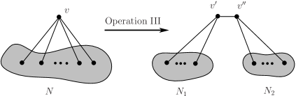
Figure 10.2: Operation III

Next, they proved that any $(k,\ell)$-minimum connected graph can be obtained from a $(k,\ell)$-initial graph.

Theorem 10.2

[73] Any $(k,\ell)$-minimum connected graph can be obtained from a $(k,\ell)$-initial graph by doing a sequence of Operations I, II and III on the initial graph.

11 Concluding remarks

As we mentioned before, the pendant tree-connectivity and path-connectivity are also nice and natural generalizations of the classical connectivity, and they have very close relation with the generalized (edge-)connectivity. However, in order to make things clear (not to cause confusion), in this survey we only concentrate on one kind of generalization, i.e., the generalized (edge-)connectivity. Actually, for the pendant tree-connectivity and path-connectivity, there have been many results published recently. For these results we refer the reader to [50, 51, 98, 99, 100].

References

- [1] N. Achuthan, N.R. Achuthan, L. Caccetta, On the Nordhaus-Gaddum problems, Australasian J. Combin. 2(1990), 5–27.
- [2] S.B. Akers, B. Krishnamurthy, A group-theoretic model for symmetric interconnection networks, IEEE Trans. Comput. 38(4)(1989), 555–566.
- [3] Y. Alavi, J. Mitchem, The connectivity and edge-connectivity of complementary graphs, Lecture Notes Math. 186(1971), 1–3.
- [4] M. Aouchiche, P. Hansen, A survey of Nordhaus-Gaddum type relations, Discrete Appl. Math. 161(4-5)(2013), 466–546.
- [5] L. Babai, Automorphism groups, isomorphism, reconstruction, in: R.L. Graham et al. (Eds.), Handbook of Combinatorics, Elsevier Science, Amsterdam, 1995, 1449–1540.
- [6] F. Bao, Y. Igarashi, S.R. Öhring, Reliable broadcasting in product networks, Discrete Appl. Math. 83(1998), 3–20.
- [7] B. Barden, R. Libeskind-Hadas, J. Davis, W. Williams, On edge-disjoint spanning trees in hypercubes, Inform. Proc. Lett. 70(1999), 13–16.
- [8] P. Bártfai, Solution of a problem proposed by P. Erdös (in Hungarian), Mat. Lapok. (1960), 175–140.
- [9] D. Bauer, H. Broersma, E. Schmeichel, Toughness in graphs: A survey, Graphs & Combin. 22(2006), 1–35.
- [10] L.W. Beineke, R.J. Wilson, Topics in Structural Graph Theory, Cambrige University Press, 2013.
- [11] L.W. Beineke, O.R. Oellermann, R.E. Pippert, The average connectivity of a graph, Discrete Math. 252(2002), 31–45.
- [12] N. Biggs, Algebraic Graph Theory, Cambridge University Press, New York, 1992.
- [13] A. Blasiak, R. Kleinberg, E. Lubetzky, Lexicographic products and the power of non-linear network coding, FOCS (2011), 609–618.
- [14] F.T. Boesch, S. Chen, A generalization of line connectivity and optimally invulnerable graphs, SIAM J. Appl. Math. 34(1078), 657–665.
- [15] B. Bollobás, Extremal Graph Theory, Acdemic press, 1978.
- [16] B. Bollobás, On graphs with at most three independent paths connecting any two vertices, Studia Sci. Math. Hungar. 1(1966), 137–140.
- [17] B. Bollobás, Cycles and semi-topological configurations, in: “Theory and Applications of graphs” (Y. Alavi and D.R. Lick, eds) Lecture Notes Math. 642, Springer, 1978, 66–74.
- [18] B. Bollobás, Random Graphs, Cambridge University Press, 2001.
- [19] B. Bollobás, A. Thomason, Random graphs of small order, in Random Graphs, Ann. Discrete. Math. (1985), 47–97.
- [20] J.A. Bondy, U.S.R. Murty, Graph Theory, GTM 244, Springer, 2008.
- [21] P. Catlin, Z. Chen, E. Palmer, On the edge-arboricity of a random graph, Ars Combin. 35(A)(1993), 129–134.
- [22] P. Catlin, J. Grossman, A. Hobbs, H. Lai, Fractional arboricity, strength, and principal partitions in graphs and matroids, Discrete Appl. Math. 40(1992), 285–302.
- [23] G. Chartrand, S. Kappor, L. Lesniak, D. Lick, Generalized connectivity in graphs, Bull. Bombay Math. Colloq. 2(1984), 1–6.
- [24] G. Chartrand, F. Okamoto, P. Zhang, Rainbow trees in graphs and generalized connectivity, Networks 55(4)(2010), 360–367.
- [25] G. Chartrand, M. Steeart, The connectivity of line graphs, Math. Ann. 182(1969), 170–174.
- [26] L. Chen, X. Li, M. Liu, Y. Mao, A solution to a conjecture on the generalized connectivity of graphs, arXiv:1304.6153 [math.CO] 2013.
- [27] X. Chen, X. Li, H. Lian, Note on packing of edge-disjoint spanning trees in sparse random graphs, arXiv:1301.1097 [math.CO] 2013.
- [28] X. Cheng, D. Du, Steiner Trees in Industry, Kluwer Academic Publisher, Dordrecht, 2001.
- [29] W. Chiue, B. Shieh, On connectivity of Cartesian product of two graphs, Appl. Math. Comput. 102(1999), 129–137.
- [30] W. Cunningham, Optimal attack and reinforcement of a netwok, J. 32(1985), 549–561.
- [31] K. Day, A.E. Al-Ayyoub, The cross product of interconnection networks, IEEE Trans. Parallel & Distributed Systems 8(2)(1997), 109–118.
- [32] D.P. Day, O.R. Oellermann, H.C. Swart, The -connectivity function of trees and complete multipartite graphs, J. Combin. Math. Combin. Comput. 10(1991), 183–192.
- [33] G.A. Dirac, In abstrakten graphen vorhandene vollständige 4-graphen und ihre unterteilungen, Math. Nach 22(1960), 61–85.
- [34] D. Du, X. Hu, Steiner Tree Problems in Computer Communication Networks, World Scientific, 2008.
- [35] A.H. Esfahanian, Generalized measures of fault tolerance with application to -cube networks, IEEE Trans. Computers 38(1989), 1586–1591.
- [36] M. Feng, M. Xu, K. Wang, Identifying codes of lexicographic product of graphs, Electron. J. Combin. 19(4)(2012), 56–63.
- [37] T.I. Fexner, A.M. Frieze, On the connectivity of random -orientable graphs and digraphs, Combinatorica 2(1982), 347–369.
- [38] P. Fragopoulou, S.G. Akl, Edge-disjoint spanning trees on the star network with applications to fault tolerance, IEEE Trans. Computers 45(2)(1996), 174–185.
- [39] A. Frank, T. Kiráby, M. Kriesell, On decomposing a hypergraph into connected sub-hypergraphs, Technical Report published by the Egrevdry Research Group, Budapest, Hungary, ISSN 1587-4451, 2001.
- [40] A.M. Frieze, Maximum matchings in a class of random graphs, J. Comb. Theory B 40(1986), 196–212.
- [41] A.M. Frieze, T. Luczak, Edge-disjoint spanning trees in random graphs, Per. Math. Hung. 21(1990), 35–37.
- [42] P. Gao, X. Pérez-Giménez, C.M. Sato, Arboricity and spanning-tree packing of random graphs, arXiv:1303.517[math.CO] 2013.
- [43] D.L. Goldsmith, On the second-order edge-connectivity of a graph, Congressus Numerantium 29(1980), 479–484.
- [44] D.L. Goldsmith, On the -order connectivity of a graph, Congressus Numerantium 32(1981), 375–382.
- [45] D.L. Goldsmith, B. Manval, V. Faber, Seperation of graphs into three components by removal of edges, J. Graph Theory 4(1980), 213–218.
- [46] M. Grötschel, The Steiner tree packing problem in design, Math. Program. 78(1997), 265–281.
- [47] M. Grötschel, A. Martin, R. Weismantel, Packing Steiner trees: A cutting plane algorithm and commputational results, Math. Program. 72(1996), 125–145.
- [48] R. Gu, X. Li, Y. Shi, The generalized 3-connectivity of random graphs, Acta Math. Sin. 57(2)(2014), 321–330.
- [49] D. Gusfield, Connectivity and edge-disjoint spanning trees, Infor. Process. Lett. 16(1983), 87–89.
- [50] M. Hager, Pendant tree-connectivity, J. Comb. Theory 38(1985), 179–189.
- [51] M. Hager, Path-connectivity in graphs, Discrete Math. 59(1986), 53–59.
- [52] R. Hammack, W. Imrich, S. Klavz̆r, Handbook of Product Graphs, Secend Edition, CRC Press, 2011.
- [53] F. Harary, The maximum connectivity of a graph, Proc. Nat. Acad. Sci. USA, 1142–1146.
- [54] A. Hellwig, L. Volkmann, The connectivity of a graph and its complement, Discrete Appl. Math. 156(2008), 3325–3328.
- [55] M.C. Heydemann, Cayley graphs and interconnection networks, in: G. Hahn and G. Sabidussi eds., Graph Symmetry, Kluwer Academic Publishing, Dordrecht, 1997, 167–224.
- [56] H.R. Hind, O.R. Oellermann, Menger-type results for three or more vertices, Congressus Numerantium 113(1996), 179–204.
- [57] A. Itai, M. Rodeh, The multi-tree approach to reliability in distributed networks, Infor. & Comput. 79(1988), 43–59.
- [58] G. Ivchenko, The strength of connectivity of a random graph, Theory Probab. Appl. 18(2009), 396–403.
- [59] K. Jain, M. Mahdian, M. Salavatipour, Packing Steiner trees, in: Proc. 14th - symposium on Discterte Algorithms, Baltimore, 2003, 266–274.
- [60] S. Klavžar, S. Špacapan, On the edge-connectivity of Cartesian product graphs, Asian-Eur. J. Math. 1(2008), 93–98.
- [61] M. Kriesell, Edge-disjoint trees containing some given vertices in a graph, J. Combin. Theory Ser. B 88(2003), 53–65.
- [62] M. Kriesell, Edge-disjoint Steiner trees in graphs without large bridges, J. Graph Theory 62(2009), 188–198.
- [63] M. Kriesell, Local spanning trees in graphs and hypergraph decomposition with respect to edge-connectivity, Technical Report 257, University of Hannover, 1999.
- [64] S. Ku, B. Wang, T. Hung, Constructing edge-disjoint spanning trees in product networks, Parallel and Distributed Systems, IEEE Transactions on parallel and disjoited systems 14(3)(2003), 213–221.
- [65] S. Lakshmivarahan, J.S. Jwo, S.K. Dhall, Symmetry in interconnection networks based on Cayley graphs of permutation groups: a survey, Parallel Comput. 19(4)(1993), 361–407.
- [66] R. Laskar, B. Auerbach, On descomposition of -partite graphs into edge-disjoint Hamilton circuits, Discrete Math. 14(1976), 265–258.
- [67] L. Lau, An approximate max-Steiner-tree-packing min-Steiner-cut theorem, Combinatorica 27(2007), 71–90.
- [68] J. Leonard, On a conjecture of Bollobás and Edrös, Period. Math. Hungar. 3(1973), 281–284.
- [69] J. Leonard, On graphs with at most four edge-disjoint paths connecting any two vertices, J. Comb. Theory Ser. B 13(1972), 242–250.
- [70] J. Leonard, Graphs with -ways, Canad. J. Math. 25(1973), 687–692.
- [71] F. Li, Z. Xu, H. Zhao, W. Wang, On the number of spanning trees of the lexicographic product of networks, Sci. China Ser. F 42(2012), 949–959.
- [72] H. Li, X. Li, Y. Mao, On extremal graphs with at most two internally disjoint Steiner trees connecting any three vertices, Bull. Malays. Math. Sci. Soc. 37(3)(2014), 747–756.
- [73] H. Li, X. Li, Y. Mao, The minimally connected graphs containing disjoint Steiner trees for given vertices, Preprint 2012.
- [74] H. Li, X. Li, Y. Mao, Y. Sun, Note on the generalized connectivity, Ars Combin. 114(2014), 193–202.
- [75] H. Li, X. Li, Y. Mao, J. Yue, Note on the spanning-tree packing number of lexicographic product graphs, Discrete Math. 338(5-6)(2015), 669–673.
- [76] H. Li, X. Li, Y. Sun, The generalied -connectivity of Cartesian product graphs, Discrete Math. Theor. Comput. Sci. 14(1)(2012), 43–54.
- [77] S. Li, Some topics on generalized connectivity of graphs, Thesis for Doctor Degree, Nankai University, 2012.
- [78] S. Li, W. Li, X. Li, The generalized connectivity of complete bipartite graphs, Ars Combin. 104(2012), 65–79.
- [79] S. Li, W. Li, X. Li, The generalized connectivity of complete equipartition -partite graphs, Bull. Malays. Math. Sci. Soc. (2)37(1)(2014), 103–121.
- [80] S. Li, X. Li, Note on the hardness of generalized connectivity, J. Comb. Optim. 24(2012), 389–396.
- [81] S. Li, X. Li, Y. Shi, The minimal size of a graph with generalized connectivity , Australasian J. Combin. 51(2011), 209–220.
- [82] S. Li, X. Li, W. Zhou, Sharp bounds for the generalized connectivity , Discrete Math. 310(2010), 2147–2163.
- [83] W. Li, On the generalized connectivity of complete multipartite graphs, Thesis for Doctor Degree, Nankai University, 2012.
- [84] X. Li, Y. Mao, Nordhaus-Gaddum-type results for the generalized edge-connectivity of graphs, Discrete Appl. Math. 185(2015), 102–112.
- [85] X. Li, Y. Mao, On extremal graphs with at most internally disjoint Steiner trees connecting any vertices, Graphs & Combin., in press.
- [86] X. Li, Y. Mao, The generalized -connectivity of lexicographic product graphs, Discrete Math. Theor. Comput. Sci. 16(1)(2014), 339–354.
- [87] X. Li, Y. Mao, The minimal size of a graph with given generalized -edge-connectivity, Ars Combin. 118(2015), 63–72.
- [88] X. Li, Y. Mao, Y. Sun, On the generalized (edge-)connectivity of graphs, Australasian J. Comb. 58(2)(2014), 304–319.
- [89] X. Li, Y. Mao, Graphs with large generalized (edge-)connectivity, arXiv: 1305.1089 [math.CO] 2013.
- [90] X. Li, J. Yue, Y. Zhao, The generalized 3-edge-connectivity of lexicographic product graphs, in Comb. Optim. Appl., LNCS 8881 (Proc. COCOA2014, Maui, HI, USA), pp.412–425.
- [91] X. Li, Y. Zhao, On graphs with only one Steiner tree connecting any vertices, arXiv:1301.4623[math.CO] 2013.
- [92] R. Libeskind-Hadas, D. Mazzoni, R. Rajagopalan, Tree-based multicasting in wormhole-routed irregular topologies, Proc. Merged 12th Int’l Parallel Processing Symp. and the Ninth Symp. Parallel and Distributed Processing, 244-249, Apr. 1998.
- [93] M. Lü, G.L. Chen, J. Xu, On super edge-connectivity of Cartesian product graphs, Networks 49(2)(2007), 135–157.
- [94] W. Mader, Ein extremalproblem des zusammenhangin endlichen graphen, Math. Z. 131(1973), 223–231.
- [95] W. Mader, Grad und lokaler zusammenhangs von graphen, Math. Ann. 205(1973), 9–11.
- [96] W. Mader, Über die maximalzahl kantendisjunkter A-Wege, Arch. Math. 30(1978), 325–336.
- [97] W. Mader, Über die maximalzahl kreuzungsfreier H-wege, Arch. Math. 31(1978), 387-402.
- [98] Y. Mao, Constructing internally disjoint pendant Steiner trees in Cartesian product networks, submitted.
- [99] Y. Mao, On the pendant tree-connectivity of graphs, submitted.
- [100] Y. Mao, Path connectivity of lexicographical product graphs, Int. J. Comput. Math., in press.
- [101] D. Matula, Determining edge-connectivity in , Proceeding of Symp. Foundation Computer Science (1987), 249–251.
- [102] C.St.J.A. Nash-Williams, Edge-disjonint spanning trees of finite graphs, J. London Math. Soc. 36(1961), 445–450.
- [103] C.St.J.A. Nash-Williams, Decomposition of finite graphs into forests, J. London Math. Soc. 39(1964), 12.
- [104] O.R. Oellermann, Connectivity and edge-connectivity in graphs: A survey, Congessus Numerantium 116(1996), 231–252.
- [105] O.R. Oellermann, On the -connectivity of a graph. Graphs & Combin. 3(1987), 285–299.
- [106] O.R. Oellermann, A note on the -connectivity function of a graph, Congessus Numerantium 60(1987), 181–188.
- [107] F. Okamoto, P. Zhang, The tree connectivity of regular complete bipartite graphs, J. Combin. Math. Combin. Comput. 74 (2010), 279–293.
- [108] K. Ozeki, T. Yamashita, Spanning trees: A survey, Graphs & Combin. 27(1)(2011), 1–26.
- [109] E. Palmer, On the spanning tree packing number of a graph: a survey, Discrete Math. 230(2001), 13–21.
- [110] E. Palmer, J. Spencer, Hitting time for edge-disjoint spanning trees in a random graph, Period. Math. Hungar. 31(1995), 151–156.
- [111] Y. Peng, C. Chen, K. Koh, On edge-toughness of a complete -partite graph, Research Report No. 304, Lee Kong Chian Centre for Mathematical Reserch, National University of Singapore, 1987.
- [112] Y. Peng, T. Tay, On edge-toughness of a graph, J. Graph Theory 17(1993), 233–246.
- [113] L. Petingi, J. Rodriguez, Bounds on the maximum number of edge-disjoint Steiner trees of a graph, Congressus Numerantium 145(2000), 43–52.
- [114] S. Rao, Graph and its complement, Proc. Indian Nat. Sci. Acad. Part A 41(1975), 297–304.
- [115] N. Robertson, P. Seymour, Graph minors . The disjoint path problems, J. Comb. Theory Ser. B 63(1995), 65–110.
- [116] J. Roskind, R. Tarjan, A Note on Finding Maximum-Cost Edge-Disjoint Spanning Trees, Math. Operations Research, 10(2)(1985), 701–708.
- [117] Sabidussi, Graphs with given group and given graph theoretical properties, Canadian J. Math. 9(1957), 515–525.
- [118] A. Schrijver, Combinatorial optimization: Polyhedra and efficiency. Vol. B, Volume 24 of Algorithms and Combinatorics, Springer-Verlag, Berlin, 2003.
- [119] N. Sherwani, Algorithms for Physical Design Automation, 3rd Edition, Kluwer Acad. Pub., London, 1999.
- [120] S. S̆pacapan, Connectivity of Cartesian products of graphs, Appl. Math. Lett. 21(2008), 682–685.
- [121] Y. Sun, X. Li, On the difference of two generalized connectivities of a graph, accepted by J. Comb. Optim.
- [122] Y. Sun, S. Zhou, Tree connectivities of Caylay graphs on Abelian groups with small degrees, accepted by Bull. Malays. Math. Sci. Soc.
- [123] B. Sørensen, C. Thomassen, On -rails in graphs, J. Comb. Theory 17(1974), 143–159.
- [124] W. Tutte, On the problem of decomposing a graph into connected factors, J. London Math. Soc. 36(1961), 221–230.
- [125] H. Wang and D. Blough, Construction of edge-disjoint spanning trees in the torus and application to multicast in wormhole-routed networks, Proc. Int’l Conf. Parallel and Distributed Computing Systems, 1999.
- [126] D. Welsh, Matroid Theorey, Academic Press, London, 1976.
- [127] D. West, H. Wu, Packing Steiner trees and -connectors in graphs, J. Comb. Theory Ser. B 102(2012), 186–205.
- [128] E.L. Wilson, R.L. Hemminger, M.D. Plimmer, A family of path properties for graphs, Math. Ann. 197(1972), 107–122.
- [129] C. Yang, J. Xu, Connectivity of lexicographic product and direct product of graphs, Ars Combin. 111(2013), 3–12.
- [130] S. Zhou, A class of arc-transitive Cayley graphs as models for interconnection networks, SIAM J. Discrete Math. 23(2009), 694–714.