Phantom crossing and quintessence limit in extended nonlinear massive gravity

Abstract

We investigate the cosmological evolution in a universe governed by the extended, varying-mass, nonlinear massive gravity, in which the graviton mass is promoted to a scalar-field. We find that the dynamics, both in flat and open universe, can lead the varying graviton mass to zero at late times, offering a natural explanation for its hugely-constrained observed value. Despite the limit of the scenario towards standard quintessence, at early and intermediate times it gives rise to an effective dark energy sector of a dynamical nature, which can also lie in the phantom regime, from which it always exits naturally, escaping a Big-Rip. Interestingly enough, although the motivation of massive gravity is to obtain an IR modification, its varying-mass extension in cosmological frameworks leads to early and intermediate times modification instead.

1 Introduction

The idea of adding mass to the graviton is quite old [1], but the necessary nonlinear terms [2] that can give rise to continuity of the observables [3, 4] lead also to Boulware-Deser (BD) ghosts [5], making the theory unstable. However, recently, a nonlinear extension of massive gravity has been constructed [6, 7] such that the Boulware-Deser ghost is systematically removed (see [8] for a review). The theoretical and phenomenological advantages, amongst which is the universe self-acceleration arising exactly from this IR gravity modification, brought this theory to a significant attention [9, 10, 11, 12, 13, 14, 15, 16, 17, 18, 19, 20, 21, 22, 23, 24, 25, 26, 27, 28, 29, 30, 31, 32, 33, 34, 35, 36, 37, 38, 39, 40, 41, 42, 43, 44, 45, 46, 47, 48, 49, 50, 51].

Despite the successes of massive gravity, in the case where the physical and the fiducial metrics have simple homogeneous and isotropic forms the theory proves to be unstable at the perturbation level [40], which led some authors to start constructing less symmetric models [13, 41]. However, in [52] a different approach was followed, that is expected to be free of the above instabilities, namely to extend the theory in a way that the graviton mass is varying, and this was achieved by introducing an extra scalar field which coupling to the graviton potentials produces an effective, varying, graviton mass.

In this work we desire to explore the cosmological implications of this “extended”, varying-mass, massive gravity, in both flat and open universe. As we show, at least in simple cosmological ansatzes, the dynamics leads the varying graviton mass to zero, or to a suitably chosen very small value in agreement with observations, at late times, and thus the theory has as a limit the standard quintessence paradigm. However, at intermediate times the varying graviton mass leads to very interesting behavior, with a dynamical effective dark energy sector which can easily lie in the phantom regime. Strictly speaking, although the motivation of massive gravity is to obtain an IR modification, its extension in cosmological frameworks leads rather to early and intermediate times modification, and thus to a radical UV modification instead.

2 Extended nonlinear massive gravity

Let us briefly review the “mass-varying massive gravity” that was recently presented in [52]. Their construction is based on the promotion of the graviton mass to a scalar-field function (potential), with the additional insertion in the action of this scalar field’s kinetic term and standard potential. Since such a modification is deeper than allowing for a varying mass, we prefer to call it “extended” nonlinear massive gravity.

In such a construction the action writes as

$$S=\int d^{4}x\sqrt{-g}\left[\frac{M_{P}^{2}}{2}R+V(\psi)(U_{2}+\alpha_{3}U_{3}+\alpha_{4}U_{4})-\frac{1}{2}\partial_{\mu}\psi\partial^{\mu}\psi-W(\psi)\right],$$ (2.1)

where $M_{p}$ is the Planck mass, $R$ the Ricci scalar, and $\psi$ is the new scalar field with $W(\psi)$ its standard potential and $V(\psi)$ its coupling potential which spontaneously breaks general covariance. Furthermore, as usual $\alpha_{3}$ and $\alpha_{4}$ are dimensionless parameters, and the graviton potentials are given by

$$U_{2}=\mathcal{K}^{\mu}_{[\mu}\mathcal{K}^{\nu}_{\nu]},\quad\quad U_{3}=\mathcal{K}^{\mu}_{[\mu}\mathcal{K}^{\nu}_{\nu}\mathcal{K}^{\rho}_{\rho]},\quad\quad U_{4}=\mathcal{K}^{\mu}_{[\mu}\mathcal{K}^{\nu}_{\nu}\mathcal{K}^{\rho}_{\rho}\mathcal{K}^{\sigma}_{\sigma]},$$ (2.2)

with $\mathcal{K}^{\mu}_{[\mu}\mathcal{K}^{\nu}_{\nu]}=(\mathcal{K}^{\mu}_{\mu}\mathcal{K}^{\nu}_{\nu}-\mathcal{K}^{\mu}_{\nu}\mathcal{K}^{\nu}_{\mu})/2$ and similarly for the other antisymmetric expressions, and

$$\mathcal{K}^{\mu}_{\nu}=\delta^{\mu}_{\nu}-\sqrt{g^{\mu\rho}f_{AB}\partial_{\rho}\phi^{A}\partial_{\nu}\phi^{B}}.$$ (2.3)

As in standard massive gravity $f_{AB}$ is a fiducial metric, and the four $\phi^{A}(x)$ are the Stückelberg scalars introduced to restore general covariance [53], and in the particular case where the $f_{AB}$ is the Minkowski metric they form Lorentz 4-vectors in the internal space and the theory presents a global Poincaré symmetry, too. Finally, one can show that the above extended massive gravity is still free of the the Boulware-Deser ghost [52].

3 Cosmological equations

Let us now examine cosmological scenarios in a universe governed by the extended nonlinear massive gravity. Firstly, in order to obtain a realistic cosmology one includes the usual matter action $S_{m}$, coupled minimally to the dynamical metric, corresponding to energy density $\rho_{m}$ and pressure $p_{m}$. Now, for simplicity we consider the fiducial metric to be Minkowski

$$f_{AB}=\eta_{AB},$$ (3.1)

and without loss of generality we assume that the dynamical and fiducial metrics are diagonalized simultaneously. For the dynamical metric one can either consider for simplicity a flat Friedmann-Robertson-Walker (FRW) form, or he can apply an open geometry. In the following two subsections we examine these two cases separately.

3.1 Flat universe

We consider a flat FRW physical metric of the form

$$d^{2}s=-N(\tau)^{2}d\tau^{2}+a(\tau)^{2}\delta_{ij}dx^{i}dx^{j},$$ (3.2)

with $N(\tau)$ the lapse function and $a(\tau)$ the scale factor, and for simplicity for the Stückelberg fields we choose the ansatz

$$\phi^{0}=b(\tau),~{}~{}~{}~{}\phi^{i}=a_{ref}x^{i},$$ (3.3)

with $a_{ref}$ a constant coefficient. Although the above specific application is only a simple subclass of the rich set of possible scenarios, it proves to exhibit very interesting cosmological behavior.

Variation of the total action $S+S_{m}$ with respect to $N$ and $a$ provides the two Friedmann equations [52]:

$$3M_{P}^{2}H^{2} = \rho_{DE}+\rho_{m},$$ (3.4)

$$-2M_{P}^{2}\dot{H} = \rho_{DE}+p_{DE}+\rho_{m}+p_{m},$$ (3.5)

where we have defined the Hubble parameter $H=\dot{a}/a$, with $\dot{a}=da/(Nd\tau)$, and in the end we set $N=1$. In the above expressions we have defined the energy density and pressure of the effective dark energy sector as

$$\rho_{DE}=\frac{1}{2}\dot{\psi}^{2}+W(\psi)+V(\psi)\left(\frac{a_{ref}}{a}-1\right)[f_{3}(a)+f_{1}(a)]\ \ \ \$$ (3.6)

$$p_{DE}=\frac{1}{2}\dot{\psi}^{2}-W(\psi)-V(\psi)f_{4}(a)-V(\psi)\dot{b}f_{1}(a),$$ (3.7)

having also introduced the convenient functions

$$f_{1}(a)=3-\frac{2a_{ref}}{a}+\alpha_{3}\left(3-\frac{a_{ref}}{a}\right)\left(1-\frac{a_{ref}}{a}\right)+\alpha_{4}\left(1-\frac{a_{ref}}{a}\right)^{2}$$

$$f_{2}(a)=1-\frac{a_{ref}}{a}+\alpha_{3}\left(1-\frac{a_{ref}}{a}\right)^{2}+\frac{\alpha_{4}}{3}\left(1-\frac{a_{ref}}{a}\right)^{3}$$

$$f_{3}(a)=3-\frac{a_{ref}}{a}+\alpha_{3}\left(1-\frac{a_{ref}}{a}\right)$$

$$f_{4}(a)=-\left[6-\frac{6a_{ref}}{a}+\left(\frac{a_{ref}}{a}\right)^{2}+\alpha_{3}\left(1-\frac{a_{ref}}{a}\right)\left(4-\frac{2a_{ref}}{a}\right)+\alpha_{4}\left(1-\frac{a_{ref}}{a}\right)^{2}\right].\ \ \ \ \$$ (3.8)

Note that from the above expressions we observe that $a_{ref}$ plays the role of a reference scale factor that can be arbitrary.

One can easily verify that the dark energy density and pressure satisfy the usual evolution equation

$$\dot{\rho}_{DE}+3H(\rho_{DE}+p_{DE})=0,$$ (3.9)

and we can also define the dark-energy equation-of-state parameter as usual as

$$w_{DE}\equiv\frac{p_{DE}}{\rho_{DE}}.$$ (3.10)

Note that in [52] the authors had named the aforementioned “dark energy” sector as “massive gravity” one, and the quantities $\rho_{DE}$ and $p_{DE}$ as $\rho_{MG}$ and $p_{MG}$. However, since in this work we focus to late time cosmological behavior, we prefer the above name.

Variation of the total action $S+S_{m}$ with respect to $\psi$ provides the scalar-field evolution equation:

$$\ddot{\psi}+3H\dot{\psi}+\frac{dW}{d\psi}+\frac{dV}{d\psi}\left[\left(\frac{a_{ref}}{a}-1\right)[f_{3}(a)+f_{1}(a)]+3\dot{b}f_{2}(a)\right]=0.\ \ \ \ \ \$$ (3.11)

Furthermore, variation of $S+S_{m}$ with respect to $b$ provides the constrain equation

$$V(\psi)Hf_{1}(a)+\dot{V}(\psi)f_{2}(a)=0.$$ (3.12)

Finally, one can also extract the matter evolution equation $\dot{\rho}_{m}+3H(\rho_{m}+p_{m})=0$.

3.2 Open universe

Let us now consider an open FRW physical metric of the form

$$d^{2}s=-N(\tau)^{2}d\tau^{2}+a(\tau)^{2}\delta_{ij}dx^{i}dx^{j}-a(\tau)^{2}\frac{k^{2}(\delta_{ij}x^{i}dx^{j})^{2}}{1+k^{2}(\delta_{ij}x^{i}x^{j})}~{},$$ (3.13)

with $N(\tau)$ the lapse function and $a(\tau)$ the scale factor, and $K<0$ with $k=\sqrt{|K|}$. For simplicity for the Stückelberg fields we choose [52]:

$$\phi^{0}=b(\tau)\sqrt{1+k^{2}(\delta_{ij}x^{i}x^{j})},~{}~{}~{}~{}\phi^{i}=kb(\tau)x^{i}~{}.$$ (3.14)

Variations of the action with respect to $N$ and $a$ give rise to the following Friedmann equations

$$3M_{P}^{2}\left(H^{2}-\frac{k^{2}}{a^{2}}\right) = \rho_{DE}+\rho_{m}~{},$$ (3.15)

$$-2M_{P}^{2}\left(\dot{H}+\frac{k^{2}}{a^{2}}\right) = \rho_{DE}+p_{DE}+\rho_{m}+p_{m},$$ (3.16)

where the effective dark energy density and pressure are given by

$$\rho_{DE}=\frac{1}{2}\dot{\psi}^{2}+W(\psi)+V(\psi)\left(\frac{kb}{a}-1\right)[f_{3}(a)+f_{1}(a)]\ \ \ \ \$$ (3.17)

$$p_{DE}=\frac{1}{2}\dot{\psi}^{2}-W(\psi)-V(\psi)f_{4}(a)-V(\psi)\dot{b}f_{1}(a),$$ (3.18)

but now the functions become

$$f_{1}(a)=3-2\frac{kb}{a}+\alpha_{3}\left(3-\frac{kb}{a}\right)\left(1-\frac{kb}{a}\right)+\alpha_{4}\left(1-\frac{kb}{a}\right)^{2}$$

$$f_{2}(a)=1-\frac{kb}{a}+\alpha_{3}\left(1-\frac{kb}{a}\right)^{2}+\frac{\alpha_{4}}{3}\left(1-\frac{kb}{a}\right)^{3}$$

$$f_{3}(a)=3-\frac{kb}{a}+\alpha_{3}\left(1-\frac{kb}{a}\right)$$

$$f_{4}(a)=-\left[6-6\frac{kb}{a}+\left(\frac{kb}{a}\right)^{2}+\alpha_{3}\left(1-\frac{kb}{a}\right)\left(4-\frac{2kb}{a}\right)+\alpha_{4}\left(1-\frac{kb}{a}\right)^{2}\right].\$$ (3.19)

These verify the usual evolution equation

$$\dot{\rho}_{DE}+3H(\rho_{DE}+p_{DE})=0.$$ (3.20)

Variation of the action with respect to the scalar field $\psi$ provides its evolution equation:

$$\ddot{\psi}+3H\dot{\psi}+\frac{dW}{d\psi}+\frac{dV}{d\psi}\left\{\left(\frac{kb}{a}-1\right)[f_{3}(a)+f_{1}(a)]+3\dot{b}f_{2}(a)\right\}=0~{}.\ \ \ \ \ \$$ (3.21)

Finally, variation with respect to $b$ provides the constraint equation

$$V(\psi)\left(H-\frac{k}{a}\right)f_{1}(a)+\dot{V}(\psi)f_{2}(a)=0~{}.$$ (3.22)

4 Cosmological behavior

The cosmological implications of extended nonlinear massive gravity, prove to be very interesting, however, at least in its present simple but general example, it can be radically different than the usual massive gravity. In the following two subsections we examine the flat and open geometry separately.

4.1 Flat universe

In the case of a flat FRW universe, the cosmological equations are (3.4), (3.5) or (3.11) and (3.12), and the reason that these equations lead to a different behavior comparing to the usual massive gravity is the constraint equation (3.12). In order to elaborate the equations we have to consider at will $W(\psi)$ and $V(\psi)$ and solve the equations to obtain $a(\tau)$, $\psi(\tau)$ and $b(\tau)$, that is the Stückelberg scalars are suitably reconstructed in order to correspond to a consistent solution.

A crucial observation is that for $f_{2}(a)\neq 0$ (which is the case in general) the constraint equation (3.12) can be explicitly solved giving

$$V(a)=C_{0}\,e^{-\int\frac{f_{1}}{af_{2}}\mathrm{d}a}=\frac{C_{0}}{(a-a_{ref})[\alpha_{4}a_{ref}^{2}-(3\alpha_{3}+2\alpha_{4})aa_{ref}+(3+3\alpha_{3}+\alpha_{4})a^{2}]},\ \ \ \ \ \$$ (4.1)

where we have used the definitions (3.8), with $C_{0}$ a positive integration constant. Thus, since from the known $V(\psi)$ we can straightforwardly obtain $\psi(V)$ as a function of $V$, relation (4.1) eventually provides $\psi(a)$. Then one can insert the known $\psi(a)$ into the Friedmann equation (3.4) which becomes a simple differential equation for $a(\tau)$ ($b(\tau)$ does not appear in (3.4)). Finally, with $a(\tau)$ known and therefore $\psi(a(\tau))$ known, one can use (3.11) to find $\dot{b}$ as

$$\dot{b}(\tau)=\frac{1}{3f_{2}(a(\tau))}\left\{-\frac{\ddot{\psi}(\tau)+3H(\tau)\dot{\psi}(\tau)+\frac{dW}{d\psi}(\tau)}{\frac{dV}{d\psi}(\tau)}-\left(\frac{a_{ref}}{a(\tau)}-1\right)\left[f_{3}(a(\tau))+f_{1}(a(\tau))\right]\right\},\ \ \ \$$ (4.2)

integration of which provides the Stückelberg-scalar function $b(\tau)$ (note however that in the observables it is $\dot{b}$ and not $b$ that appears).

A first observation that one can immediately make from (4.1) is that in general at late times the graviton mass always goes to zero, independently of the specific $V(\psi)$ and the model parameters, that is the evolution of $\psi$ will be such, in order for $V(\psi)$ to go to zero (if $V(\psi)$ cannot be zero for any $\psi$ then the scenario will break down at some scale factor, since $\psi$ would need to be complex, that is a solution cannot be found any more). This means that the present scenario of extended nonlinear massive gravity, in a cosmological framework of a flat universe, cannot provide the usual massive gravity, and on the contrary it always gives the standard gravity along with the standard quintessence scenario [54, 55]. Similarly, once introduced, the scalar-field cannot be set to zero by hand, since this is not a solution of (3.11) and (3.12) (unless we also set $V(\psi)=0$ but in this case the model coincides completely with standard quintessence), that is $\psi$ will always have a non-trivial dynamics.

However, although at late times the present scenario coincides with standard quintessence, it can have a very interesting behavior at intermediate times. In particular, the dark energy sector is not only dynamical, but it can easily lie at the phantom regime [56, 57, 58, 59, 60, 61]. This can be seen by observing $\rho_{DE}$ and $p_{DE}$ from (3.6),(3.7), which using the constraint equation (3.12) give

$$\rho_{DE}+p_{DE}=\dot{\psi}^{2}-V(\psi)\left(\dot{b}-\frac{a_{ref}}{a}\right)f_{1}(a).$$ (4.3)

So we can always find regions in the $\alpha_{3}$,$\alpha_{4}$ parameter space, that can lead to $p_{DE}+\rho_{DE}<0$ at some stage of the evolution (with a potential $W(\psi)$ that will not lead to large $\dot{\psi}$), even if we require to always have $\rho_{DE}>0$ (which does not need to be the case in general). This null energy condition violation is always canceled at late times, where the vanishing of the graviton mass leads to $w_{DE}\geq-1$.

From the above discussion however one can see that despite the interesting cosmological behavior, in the flat case there is a potential disadvantage, namely that the graviton square mass, as it is given by (4.1), diverges and changes sign at least for one finite scale factor independently of the model parameters (even if we choose $\alpha_{3}$,$\alpha_{4}$ in order for the second term in the denominator not to have roots, there is always the point $a(\tau)=a_{ref}$). A negative graviton square mass would make the scenario unstable at the perturbation level and thus its application meaningless, therefore we desire the observable universe evolution to take place in the regime $V(\psi)\geq 0$. In order to avoid a collapse of the scenario in the future (choosing $a_{ref}$ larger than the present scale factor) in the following we prefer to choose it suitably small in order not to interfere with the observed thermal history of the universe ($a_{ref}\lesssim 10^{-9}$ in order to be smaller than the Big Bang nucleosynthesis scale factor). Note also that one could additionally “shield” $a_{ref}$ with a cosmological bounce, case in which the universe is always away from it [62], or even choose $a_{ref}$ to be negative. However, these considerations can only cure the problem phenomenologically, while at the theoretical level it remains unsolved. Clearly, the scenario of a flat universe has serious disadvantages and thus one should look for a more general solution through its generalizations. This will be performed in the next subsection, where the addition of curvature makes the graviton mass square always positive. However, for completeness we provide in the present subsection the phenomenologically (but not theoretically) consistent flat analysis, too.

In order to present the above behavior in a more transparent way, we consider without loss of generality the graviton mass potential to be

$$V(\psi)=V_{0}e^{-\lambda_{V}\psi},$$ (4.4)

and the usual scalar-field potential

$$W(\psi)=W_{0}e^{-\lambda_{W}\psi}.$$ (4.5)

In this case $\psi(a)=-\ln(V(a)/V_{0})/\lambda_{V}$, with $V(a)$ given by (4.1), and thus substitution into (3.4) gives a differential equation that can be easily solved numerically to give $a(\tau)$, while insertion into (4.2) provides $\dot{b}$ and therefore all the observables are known. In Fig. 1 we present the effective dark-energy equation-of-state parameter $w_{DE}$ as a function of the redshift $z=a_{0}/a-1$ (with $a_{0}$ the present scale factor set to 1), with the reference scale factor $a_{ref}$ set to $10^{-9}$, and assuming the matter to be dust ($w_{m}\equiv p_{m}/\rho_{m}=0$ that is $\rho_{m}(a)=\rho_{m0}/a^{3}$, with $\rho_{m0}$ the energy density at present).

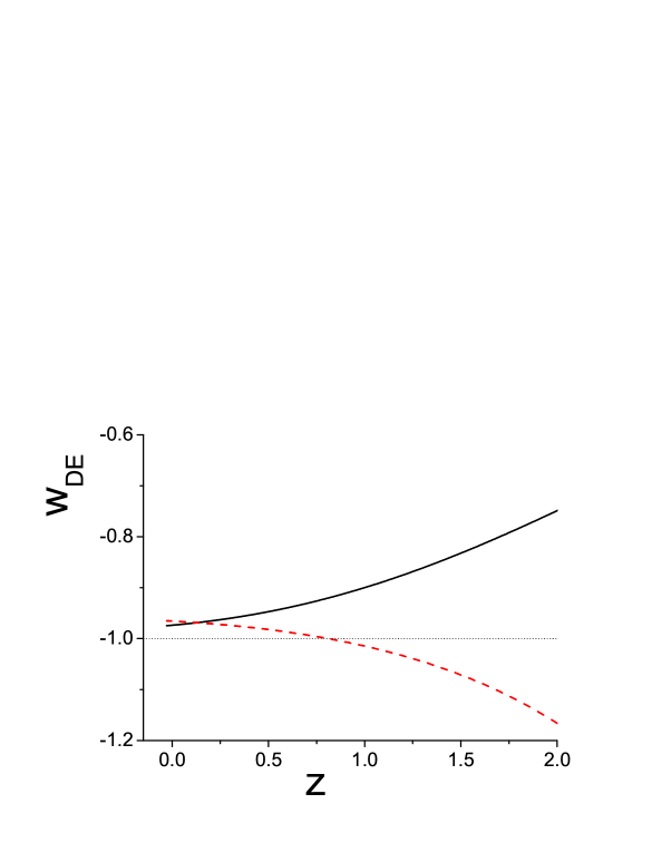
Figure 1: Evolution of the dark energy equation-of-state parameter $w_{DE}$ as a function of the redshift $z$, in a flat universe, in the case where the usual scalar field potential is $W(\psi)=W_{0}e^{-\lambda_{W}\psi}$ and the coupling potential is $V(\psi)=V_{0}e^{-\lambda_{V}\psi}$. The black-solid curve corresponds to $\alpha_{3}=2$, $\alpha_{4}=-2$, $V_{0}=1$, $W_{0}=1.2$, $C_{0}=0.001$, $\rho_{m0}=0.05$ $\lambda_{V}=0.7$, $\lambda_{W}=0.01$, $M_{P}=10$, while the red-dashed curve corresponds to $\alpha_{3}=1/3$, $\alpha_{4}=-2$, $V_{0}=10$, $W_{0}=5$, $C_{0}=0.05$, $\rho_{m0}=0.5$, $\lambda_{V}=0.5$, $\lambda_{W}=0.02$, $M_{P}=10$. All dimensional parameters are normalized in unit of $M_{P}$ given that $a_{0}=1$, and the dotted -1-line is depicted for convenience.

The parameters $\alpha_{3}$,$\alpha_{4}$,$V_{0}$,$W_{0}$,$\lambda_{V}$,$\lambda_{W}$ are chosen at will (concerning $\alpha_{3}$,$\alpha_{4}$ we have to ensure that they lead to a positive graviton square mass, that is especially to a positive last term in the denominator of (4.1)), while we fix $\rho_{m0}$ and the integration constant $C_{0}$ in order for the present dark energy density $\Omega_{DE}\equiv\rho_{DE}/(3M_{P}^{2}H^{2})$ to be $\approx 0.72$ and its initial value to be $\approx 0$ (concerning the observables no more condition is needed since it is $\dot{b}$ and not $b$ that appears in the corresponding relations, however if one desires to obtain $b(\tau)$ too then he needs to impose an extra condition, for instance the present $b$-value).

As described above, at early and intermediate times the coupling potential $V(\psi)$ is non-zero leading $w_{DE}$ to exhibit a dynamical nature, which can lie in the quintessence regime (black-solid curve) or in the phantom regime (red-dashed curve). Additionally, as we said, at late times, where the coupling $V(\psi)$ becomes zero, both sub-cases tend to their usual quintessence limit, where the final $w_{DE}$ is determined solely from the $W$-potential exponent $\lambda_{W}$ [63], with the second model experiencing the phantom-divide crossing from below to above.

In summary, as we can see the scenario at hand exhibits very interesting cosmological behavior at early and intermediate times, with a dynamical dark energy sector which can additionally lie in the phantom regime, before limit towards the standard quintessence scenario. Note that despite the phantom realization, at late times we always obtain $w_{DE}\geq-1$ since the vanishing of the graviton mass restores the null energy condition for the effective dark energy sector, that is the universe will always escape from the phantom regime and the Big-Rip future [64, 65] that is common to the majority of phantom models.

However, as we mentioned, the above flat scenario has two significant disadvantages. The first is that not all ansantzes for $V(\psi)$ can lead to consistent solutions at all times, since the field $\psi$ would need to become complex at some scale factor, that is the theory breaks down. Secondly, the appearance of $a_{ref}$ in the equations leads to scale-factor regions where the graviton mass square becomes negative, and thus the theory becomes unstable at the perturbation level. Although one can still cure the above problems at the phenomenological level, and move them away from the observed universe history, clearly a generalization of the scenario is necessary in order to completely remove these disadvantages. This is performed if one goes beyond the flat case, as we analyze in the next subsection.

4.2 Open universe

In the previous section we investigated extended massive gravity in the case of a flat FRW universe, and we saw that the resulting cosmological behavior can be very interesting. Although we chose the reference scale factor $a_{ref}$ to be suitably small in order for the graviton mass square to be always positive during the observed universe history, it is desirable to consider a generalization of the scenario, where the potential problem of the graviton mass square negativity will be completely absent. This is obtained by applying extended massive gravity in a non-flat geometry.

In the case of an open FRW universe, the cosmological equations are (3.15), (3.16) or (3.21) and (3.22) (note that in this case there is no need for a reference scale factor, since it has been absorbed inside $b(\tau)$). One difference comparing to the flat case is that the constraint equation (3.22) cannot be solved analytically and thus it has to be considered along the other cosmological equations. Although this brings an additional mathematical complexity, it offers a great physical advantage, since the constraint satisfaction can be obtained by significantly larger solution subclasses, and therefore one can always, and in general, find solutions where the graviton mass square is always positive and finite. Similarly to the flat case, in the following we consider at will the usual scalar field potential $W(\psi)$ and the coupling potential $V(\psi)$ and we solve the equations to obtain $a(\tau)$, $\psi(\tau)$ and $b(\tau)$.

Let us consider known forms for $W(\psi)$ and $V(\psi)$. Due to the constraint dependence on $b(\tau)$ it cannot be solved alone, and thus one needs to solve the whole system of equations simultaneously. Since this is not analytically possible we proceed to a numerical elaboration of a specific example. In particular, we first solve algebraically (and analytically if it is possible) the constraint (3.22) in order to extract $b(\tau)$ as a function of $a(\tau)$,$\dot{a}(\tau)$,$\psi(\tau)$,$\dot{\psi}(\tau)$ and then substituting the resulting (quite complicated) expression into (3.15),(3.16) we obtain two differential equations for $a(\tau)$ and $\psi(\tau)$ that do not depend on $b(\tau)$, which can be numerically solved. Note that contrary to the flat case $V(\psi)$ does not need to be able to become zero at some $\psi$ in order for the equations to be solvable, however for phenomenological reasons we do consider it to be able to reach zero or very small values chosen at will and in agreement with experimental bounds (thus in this case one can re-obtain the usual non-flat massive gravity, where the graviton mass is very small but non-zero).

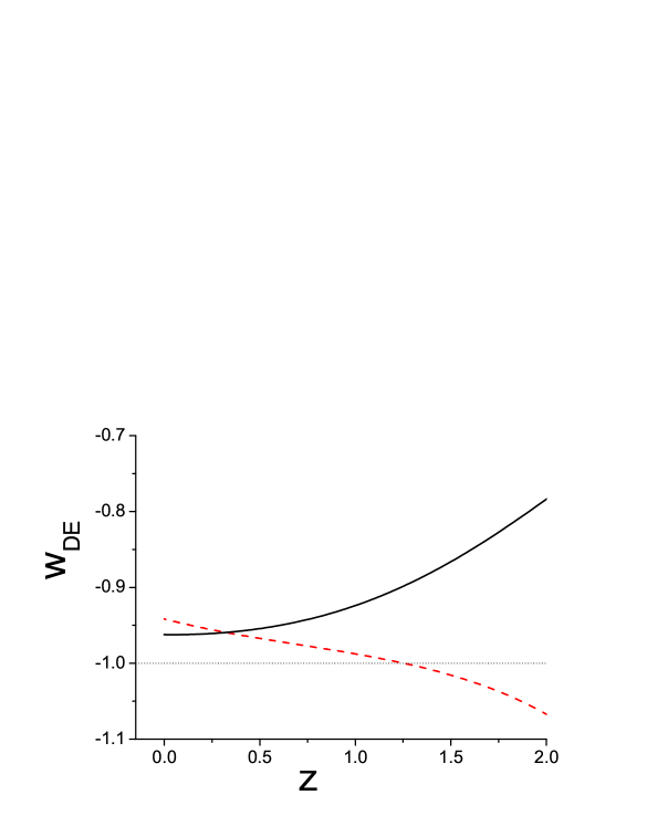
Figure 2: Evolution of the dark energy equation-of-state parameter $w_{DE}$ as a function of the redshift $z$, in an open universe, in the case where the usual scalar field potential is $W(\psi)=W_{0}e^{-\lambda_{W}\psi}$ and the coupling potential is $V(\psi)=V_{0}e^{-\lambda_{V}\psi}$. The black-solid curve corresponds to $\alpha_{3}=1$, $\alpha_{4}=1$, $k=0.02$, $V_{0}=0.6$, $W_{0}=0.4$, $\rho_{m0}=0.09$, $\lambda_{V}=6$, $\lambda_{W}=0.4$, $M_{P}=1$ (with $\dot{a}_{0}=0.3$, $\psi_{0}=1.7$, $\dot{\psi_{0}}=0.09$) while the red-dashed curve corresponds to $\alpha_{3}=2$, $\alpha_{4}=2$, $k=0.3$, $V_{0}=2.4$, $W_{0}=4$, $\rho_{m0}=0.04$, $\lambda_{V}=5.5$, $\lambda_{W}=0.6$, $M_{P}=1$ (with $\dot{a}_{0}=0.9$, $\psi_{0}=1.5$, $\dot{\psi_{0}}=0.33$). All dimensional parameters are normalized in unit of $M_{P}$ given that $a_{0}=1$, and the dotted -1-line is depicted for convenience.

We choose both $V(\psi)$ and $W(\psi)$ to have the exponential forms (4.4) and (4.5), namely $V(\psi)=V_{0}e^{-\lambda_{V}\psi}$ and $W(\psi)=W_{0}e^{-\lambda_{W}\psi}$ respectively, although we could still add a constant in $V(\psi)$, suitably small in order to be consistent with experimental bounds. We evolve the system numerically, using the redshift $z=a_{0}/a-1$ as the independent variable (with $a_{0}=1$ the present scale factor), and assuming dust matter ($\rho_{m}(a)=\rho_{m0}/a^{3}$, with $\rho_{m0}$ the present energy density). The parameters $\alpha_{3}$,$\alpha_{4}$,$V_{0}$,$\lambda_{V}$,$W_{0}$,$\lambda_{W}$ are chosen at will, while we fix $k$ in order for the present curvature density parameter ($\Omega_{k}=k^{2}/(a^{2}H^{2})$) to be $0.01$, and we fix the present values $\rho_{m0}$, $\psi_{0}$, $\dot{\psi}_{0}$ and $\dot{a}_{0}$ in order for the present dark energy density $\Omega_{DE}\equiv\rho_{DE}/(3M_{P}^{2}H^{2})$ to be $\approx 0.72$, its initial value to be $\approx 0$, and the present dark-energy equation-of-state parameter to be between $-0.9$ and $-1$ in agreement with observations.

In fig. 2 we present $w_{DE}$ as a function of $z$, for two choices of the parameters. As we observe, at early and intermediate times the coupling potential $V(\psi)$ is non-zero leading $w_{DE}$ to exhibit a dynamical nature, which can lie in the quintessence regime (black-solid curve) or in the phantom regime (red-dashed curve), and it can cross the phantom divide from below to above, before asymptotically limit towards the usual quintessence scenario. This behavior is similar to the flat universe, however as we mentioned, in the present case the graviton mass square is always finite and positive, independently of the specific solution.

5 Discussion

In this work we investigated the cosmological evolution in a universe governed by the extended, varying-mass, nonlinear massive gravity. Even for simple ansatzes the scenario proves to have a very interesting behavior, comparing with standard massive gravity.

The first result is that the dynamics in cosmological frameworks can lead the varying graviton mass to zero at late times, both in flat and open geometry (in the open case one can also obtain at will a non-zero but suitably small value if he correspondingly choose the coupling potential), and thus the theory possesses as a limit the standard quintessence paradigm. This is a great advantage of the present construction, since it offers a natural explanation of the tiny and hugely-constrained graviton mass that arises from current observations. The graviton mass does not have to be tuned to an amazingly small number, as it is the case in standard massive gravity, but it is the dynamics that can lead it asymptotically to zero. Additionally, although in the simple flat case one may face the problem of a divergent or negative graviton mass square, which should be then shielded by a cosmological bounce, in the non-flat scenario the graviton mass square is always finite and positive, independently of the specific solution.

Despite the vanishing of the graviton mass at late times, and the limit of the scenario towards standard quintessence, at early and intermediate ones it can lead to very interesting behavior. In particular, it can give rise to an effective dark energy sector of a dynamical nature, which can also lie in the phantom regime. The violation of the null energy condition for the effective dark energy sector at intermediate times arises naturally for suitable (not fine-tuned) regions in the Lagrangian parameters, and it is always canceled at late times due to the vanishing of the graviton mass. These features are in agreement with observations and they offer an explanation for the dynamical evolution of the dark-energy equation-of-state parameter, for its relaxation close or at the cosmological constant value, and also for the indicated possibility to have crossed the phantom divide. Moreover, even if it enters the phantom regime, the scenario at hand always returns naturally to the quintessence one, offering a solution to the Big-Rip fate of the standard phantom scenarios. The complete investigation of the possible late-time behaviors is performed in [66], through a detailed dynamical analysis.

We mention here that although we performed the above analysis with the fiducial metric to be Minkowksi, and with specific ansantzes for the potentials and the Stückelberg-scalars, qualitatively the obtained behavior is not a result of them, but it arises from the deeper structure of the theory, namely from the scalar-field coupling to the graviton potential. Thus, we do not expect the results to change in more general cases, unless one fine-tunes the theory.

In the above analysis we remained at the background level, as a first approach to the examination of the properties of the theory. Obviously, a crucial issue is the complete investigation of the perturbations, in order to see whether the scenario at hand suffers from instabilities. Although one could be based on similar studies of usual massive gravity [22, 28, 40, 44, 46], and see that the generalized Higuchi bound is satisfied, we mention that since a cosmic scalar is introduced to drive the graviton mass varying along background evolution, the stability issue arisen from this scalar field ought to be taken into account in a global analysis. Such a complete perturbation analysis of the extended nonlinear massive gravity lies beyond the scope of the present work and it is left for future investigation.

In conclusion, the extended, varying-mass, nonlinear massive gravity leads to very interesting cosmological behavior at early and intermediate times, while it limits towards the standard quintessence scenario, where the graviton is massless and the extra scalar is only minimally coupled to gravity. Strictly speaking, although the motivation of massive gravity is to obtain an IR modification, its varying-mass extension in cosmological frameworks leads rather to early and intermediate times modification, and thus to a UV modification instead.

Acknowledgments

We wish to thank Y-F. Cai, A. Gumrukcuoglu, Q-G. Huang, T. Koivisto, C. Lin, S. Mukohyama, Y.-S, Piao, J. Stokes, N. Tamanini and S.-Y. Zhou, for useful comments. The research project is implemented within the framework of the Action «Supporting Postdoctoral Researchers» of the Operational Program “Education and Lifelong Learning” (Action’s Beneficiary: General Secretariat for Research and Technology), and is co-financed by the European Social Fund (ESF) and the Greek State.

References

- [1] M. Fierz, W. Pauli, On relativistic wave equations for particles of arbitrary spin in an electromagnetic field, Proc. Roy. Soc. Lond. A173, 211 (1939).
- [2] A. I. Vainshtein, To the problem of nonvanishing gravitation mass, Phys. Lett. B 39, 393 (1972).
- [3] H. van Dam, M. J. G. Veltman, Massive and massless Yang-Mills and gravitational fields, Nucl. Phys. B22, 397 (1970).
- [4] V. I. Zakharov, Linearized gravitation theory and the graviton mass, JETP Lett. 12, 312 (1970).
- [5] D. G. Boulware, S. Deser, Can gravitation have a finite range?, Phys. Rev. D6, 3368 (1972).
- [6] C. de Rham, G. Gabadadze, Generalization of the Fierz-Pauli Action, Phys. Rev. D82, 044020 (2010), [arXiv:1007.0443].
- [7] C. de Rham, G. Gabadadze and A. J. Tolley, Resummation of Massive Gravity, Phys. Rev. Lett. 106, 231101 (2011), [arXiv:1011.1232].
- [8] K. Hinterbichler, Theoretical Aspects of Massive Gravity, Rev. Mod. Phys. 84, 671 (2012), [arXiv:1105.3735].
- [9] K. Koyama, G. Niz and G. Tasinato, Strong interactions and exact solutions in non-linear massive gravity, Phys. Rev. D 84 (2011) 064033, [arXiv:1104.2143].
- [10] S. F. Hassan and R. A. Rosen, Resolving the Ghost Problem in non-Linear Massive Gravity, Phys. Rev. Lett. 108, 041101 (2012), [arXiv:1106.3344].
- [11] C. de Rham, G. Gabadadze and A. Tolley, Ghost free Massive Gravity in the Stúckelberg language, Phys. Lett. B 711, 190 (2012), [arXiv:1107.3820].
- [12] B. Cuadros-Melgar, E. Papantonopoulos, M. Tsoukalas and V. Zamarias, Massive Gravity with Anisotropic Scaling, [arXiv:1108.3771].
- [13] G. D’Amico, C. de Rham, S. Dubovsky, G. Gabadadze, D. Pirtskhalava, A. J. Tolley, Massive Cosmologies, [arXiv:1108.5231].
- [14] S. F. Hassan and R. A. Rosen, Bimetric Gravity from Ghost-free Massive Gravity, JHEP 1202, 126 (2012), [arXiv:1109.3515].
- [15] J. Kluson, Note About Hamiltonian Structure of Non-Linear Massive Gravity, JHEP 1201, 013 (2012), [arXiv:1109.3052].
- [16] A. E. Gumrukcuoglu, C. Lin and S. Mukohyama, Open FRW universes and self-acceleration from nonlinear massive gravity, JCAP 1111, 030 (2011), [arXiv:1109.3845].
- [17] M. S. Volkov, Cosmological solutions with massive gravitons in the bigravity theory, JHEP 1201, 035 (2012), [arXiv:1110.6153].
- [18] M. von Strauss, A. Schmidt-May, J. Enander, E. Mortsell and S. F. Hassan, Cosmological Solutions in Bimetric Gravity and their Observational Tests, JCAP 1203, 042 (2012), [arXiv:1111.1655].
- [19] D. Comelli, M. Crisostomi, F. Nesti and L. Pilo, FRW Cosmology in Ghost Free Massive Gravity, JHEP 1203, 067 (2012) [Erratum-ibid. 1206, 020 (2012)], [arXiv:1111.1983].
- [20] S. F. Hassan and R. A. Rosen, Confirmation of the Secondary Constraint and Absence of Ghost in Massive Gravity and Bimetric Gravity, JHEP 1204, 123 (2012), [arXiv:1111.2070].
- [21] L. Berezhiani, G. Chkareuli, C. de Rham, G. Gabadadze and A. J. Tolley, On Black Holes in Massive Gravity, Phys. Rev. D 85, 044024 (2012), [arXiv:1111.3613].
- [22] A. E. Gumrukcuoglu, C. Lin and S. Mukohyama, Cosmological perturbations of self-accelerating universe in nonlinear massive gravity, JCAP 1203, 006 (2012), [arXiv:1111.4107].
- [23] N. Khosravi, N. Rahmanpour, H. R. Sepangi and S. Shahidi, Multi-Metric Gravity via Massive Gravity, Phys. Rev. D 85, 024049 (2012), [arXiv:1111.5346].
- [24] Y. Brihaye and Y. Verbin, Perfect Fluid Spherically-Symmetric Solutions in Massive Gravity, [arXiv:1112.1901].
- [25] I. L. Buchbinder, D. D. Pereira and I. L. Shapiro, One-loop divergences in massive gravity theory, Phys. Lett. B 712, 104 (2012), [arXiv:1201.3145].
- [26] H. Ahmedov and A. N. Aliev, Type N Spacetimes as Solutions of Extended New Massive Gravity, Phys. Lett. B 711, 117 (2012), [arXiv:1201.5724].
- [27] E. A. Bergshoeff, J. J. Fernandez-Melgarejo, J. Rosseel and P. K. Townsend, On ’New Massive’ 4D Gravity, JHEP 1204, 070 (2012), [arXiv:1202.1501].
- [28] M. Crisostomi, D. Comelli and L. Pilo, Perturbations in Massive Gravity Cosmology, [arXiv:1202.1986].
- [29] M. F. Paulos and A. J. Tolley, Massive Gravity Theories and limits of Ghost-free Bigravity models, [arXiv:1203.4268].
- [30] S. F. Hassan, A. Schmidt-May and M. von Strauss, Proof of Consistency of Nonlinear Massive Gravity in the Stúckelberg Formulation, [arXiv:1203.5283].
- [31] D. Comelli, M. Crisostomi, F. Nesti and L. Pilo, Degrees of Freedom in Massive Gravity, [arXiv:1204.1027].
- [32] F. Sbisa, G. Niz, K. Koyama and G. Tasinato, Characterising Vainshtein Solutions in Massive Gravity, [arXiv:1204.1193].
- [33] J. Kluson, Non-Linear Massive Gravity with Additional Primary Constraint and Absence of Ghosts, [arXiv:1204.2957].
- [34] G. Tasinato, K. Koyama and G. Niz, New symmetries in Fierz-Pauli massive gravity, [arXiv:1204.5880].
- [35] K. Morand and S. N. Solodukhin, Dual Massive Gravity, [arXiv:1204.6224].
- [36] V. F. Cardone, N. Radicella and L. Parisi, Constraining massive gravity with recent cosmological data, Phys. Rev. D 85, 124005 (2012), [arXiv:1205.1613].
- [37] V. Baccetti, P. Martin-Moruno and M. Visser, Massive gravity from bimetric gravity, [arXiv:1205.2158].
- [38] P. Gratia, W. Hu and M. Wyman, Self-accelerating Massive Gravity: Exact solutions for any isotropic matter distribution, [arXiv:1205.4241].
- [39] M. S. Volkov, Exact self-accelerating cosmologies in the ghost-free bigravity and massive gravity, [arXiv:1205.5713].
- [40] A. De Felice, A. E. Gumrukcuoglu and S. Mukohyama, Massive gravity: nonlinear instability of the homogeneous and isotropic universe, [arXiv:1206.2080].
- [41] A. E. Gumrukcuoglu, C. Lin and S. Mukohyama, Anisotropic Friedmann-Robertson-Walker universe from nonlinear massive gravity, [arXiv:1206.2723].
- [42] C. de Rham and S. Renaux-Petel, Massive Gravity on de Sitter and Unique Candidate for Partially Massless Gravity, [arXiv:1206.3482].
- [43] M. Berg, I. Buchberger, J. Enander, E. Mortsell and S. Sjors, Growth Histories in Bimetric Massive Gravity, [arXiv:1206.3496].
- [44] G. D’Amico, Cosmology and perturbations in massive gravity, [arXiv:1206.3617].
- [45] V. Baccetti, P. Martin-Moruno and M. Visser, Null Energy Condition violations in bimetric gravity, [arXiv:1206.3814].
- [46] M. Fasiello and A. J. Tolley, Cosmological perturbations in Massive Gravity and the Higuchi bound, [arXiv:1206.3852].
- [47] G. D’Amico, G. Gabadadze, L. Hui and D. Pirtskhalava, Quasi-Dilaton: Theory and Cosmology, [arXiv:1206.4253].
- [48] V. Baccetti, P. Martin-Moruno and M. Visser, Gordon and Kerr-Schild ansatze in massive and bimetric gravity, [arXiv:1206.4720].
- [49] Y. -F. Cai, D. A. Easson, C. Gao and E. N. Saridakis, Charged black holes in nonlinear massive gravity, [arXiv:1211.0563].
- [50] D. Langlois and A. Naruko, Cosmological solutions of massive gravity on de Sitter, [arXiv:1206.6810].
- [51] C. de Rham, G. Gabadadze, L. Heisenberg and D. Pirtskhalava, Non-Renormalization and Naturalness in a Class of Scalar-Tensor Theories, [arXiv:1212.4128].
- [52] Q. -G. Huang, Y. -S. Piao and S. -Y. Zhou, Mass-Varying Massive Gravity, [arXiv:1206.5678].
- [53] N. Arkani-Hamed, H. Georgi and M. D. Schwartz, Effective field theory for massive gravitons and gravity in theory space, Annals Phys. 305, 96 (2003), [arXiv:hep-th/0210184].
- [54] P. J. E. Peebles and B. Ratra, Cosmology with a Time Variable Cosmological Constant, Astrophys. J. 325, L17 (1988).
- [55] C. Wetterich, Cosmology and the Fate of Dilatation Symmetry, Nucl. Phys. B 302, 668 (1988).
- [56] R. R. Caldwell, A Phantom menace?, Phys. Lett. B 545, 23 (2002), [arXiv:astro-ph/9908168].
- [57] M. P. Dabrowski, T. Stachowiak and M. Szydlowski, Phantom cosmologies, Phys. Rev. D 68, 103519 (2003), [arXiv:hep-th/0307128].
- [58] X. -m. Chen, Y. -g. Gong and E. N. Saridakis, Phase-space analysis of interacting phantom cosmology, JCAP 0904, 001 (2009), [arXiv:0812.1117].
- [59] E. N. Saridakis, Phantom evolution in power-law potentials, Nucl. Phys. B 819, 116 (2009), [arXiv:0902.3978].
- [60] Y. -F. Cai, E. N. Saridakis, M. R. Setare and J. -Q. Xia, Quintom Cosmology: Theoretical implications and observations, Phys. Rept. 493, 1 (2010), [arXiv:0909.2776].
- [61] E. N. Saridakis and S. V. Sushkov, Quintessence and phantom cosmology with non-minimal derivative coupling, Phys. Rev. D 81, 083510 (2010), [arXiv:1002.3478].
- [62] Y. -F. Cai, C. Gao and E. N. Saridakis, Bounce and cyclic cosmology in extended nonlinear massive gravity, JCAP 1210, 048 (2012), [arXiv:1207.3786].
- [63] E. J. Copeland, A. RLiddle and D. Wands, Exponential potentials and cosmological scaling solutions, Phys. Rev. D 57, 4686 (1998), [arXiv:gr-qc/9711068].
- [64] F. Briscese, E. Elizalde, S. Nojiri and S. D. Odintsov, Phantom scalar dark energy as modified gravity: Understanding the origin of the Big Rip singularity, Phys. Lett. B 646, 105 (2007), [arXiv:hep-th/0612220].
- [65] S. Capozziello, M. De Laurentis, S. Nojiri and S. D. Odintsov, Classifying and avoiding singularities in the alternative gravity dark energy models, Phys. Rev. D 79, 124007 (2009), [arXiv:0903.2753].
- [66] G. Leon, J. Saavedra and E. N. Saridakis, Cosmological behavior in extended nonlinear massive gravity, [arXiv:1301.7419].