Local and global Fokker-Planck neoclassical calculations showing flow and bootstrap current modification in a pedestal

Abstract

In transport barriers, particularly H-mode edge pedestals, radial scale lengths can become comparable to the ion orbit width, causing neoclassical physics to become radially nonlocal. In this work, the resulting changes to neoclassical flow and current are examined both analytically and numerically. Steep density gradients are considered, with scale lengths comparable to the poloidal ion gyroradius, together with strong radial electric fields sufficient to electrostatically confine the ions. Attention is restricted to relatively weak ion temperature gradients (but permitting arbitrary electron temperature gradients), since in this limit a $\delta f$ (small departures from a Maxwellian distribution) rather than full-$f$ approach is justified. This assumption is in fact consistent with measured inter-ELM H-Mode edge pedestal density and ion temperature profiles in many present experiments, and is expected to be increasingly valid in future lower collisionality experiments. In the numerical analysis, the distribution function and Rosenbluth potentials are solved for simultaneously, allowing use of the exact field term in the linearized Fokker-Planck-Landau collision operator. In the pedestal, the parallel and poloidal flows are found to deviate strongly from the best available conventional neoclassical prediction, with large poloidal variation of a different form than in the local theory. These predicted effects may be observable experimentally. In the local limit, the Sauter bootstrap current formulae appear accurate at low collisionality, but they can overestimate the bootstrap current near the plateau regime. In the pedestal ordering, ion contributions to the bootstrap and Pfirsch-Schlüter currents are also modified.

I Introduction

Neoclassical effects in a plasma – the flows, fluxes, and currents determined by collisions in a toroidal equilibrium in the absence of turbulence – set a minimum level of radial transport Hinton F L and Hazeltine R D (1976); Helander P and Sigmar D J (2002). In transport barriers – the pedestal at the edge of an H-mode or internal transport barriers – neoclassical effects are particularly important for several reasons. First, the pressure gradient driven flows and bootstrap current (thought to be determined or at least strongly influenced by neoclassical physics even in the presence of turbulence) become large due to the small radial scale-lengths. Second, turbulent radial transport is reduced, so neoclassical radial transport becomes more relevant. Both the flows and bootstrap current will affect the global stability of the transport barrier region. For example, to predict whether given plasma profiles are stable to Edge Localized Modes (ELMs) and to predict the nature of such ELMs Snyder P B and Wilson H R (2003), accurate calculation of the bootstrap current is essential.

However, conventional neoclassical calculations are not formally valid in the pedestal. The reason is that in conventional neoclassical calculations, the main ion distribution function $f_{\mathrm{i}}$ is expanded in an asymptotic seriesHinton F L and Hazeltine R D (1976); Helander P and Sigmar D J (2002) $f_{\mathrm{i}}=f_{\mathrm{Mi}}+f_{1}+\ldots$ with $f_{1}/f_{\mathrm{Mi}}\sim\rho_{\theta}/r_{\bot}\ll 1$, where $f_{\mathrm{Mi}}$ is a Maxwellian, $\rho_{\theta}=(B/B_{\theta})v_{\mathrm{i}}/\Omega$ is the poloidal ion gyroradius, $B=|\mbox{\boldmath$B$}|$ is the magnitude of the magnetic field, $B_{\theta}$ is the poloidal magnetic field, $r_{\bot}\sim|\nabla\ln p_{\mathrm{i}}|^{-1}\sim|\nabla\ln T_{\mathrm{i}}|^{-1}$ is the scale-length of ion pressure $p_{\mathrm{i}}$ or ion temperature $T_{\mathrm{i}}$, $v_{\mathrm{i}}=\sqrt{2T_{\mathrm{i}}/m_{\mathrm{i}}}$ is the ion thermal speed, $\Omega=ZeB/(m_{\mathrm{i}}c)$ is the gyrofrequency, $Z$ is the ion charge in units of the proton charge $e$, $m_{\mathrm{i}}$ is the ion mass, and $c$ is the speed of light. In the pedestal, $r_{\bot}$ is observed to be comparable to $\rho_{\theta}$ in present experiments. In particular, the density gradient scale length is generally comparable to $\rho_{\theta}$. (For this discussion it does not matter whether $r_{\bot}$ actually scales with $\rho_{\theta}$.) The first two terms in the asymptotic series $f_{\mathrm{Mi}}$ and $f_{1}$ are then of comparable magnitude, so the asymptotic approach breaks down. In the conventional case, the orbit width ($\sim\rho_{\theta}$) is thin compared to the equilibrium profiles, so neoclassical effects are radially local: the flows on a given flux surface depend only on the physical quantities and their radial gradients at that surface. However, in a transport barrier where the ion orbit width is not small relative to the equilibrium scales, the ions will sample a range of densities and temperatures during their orbits. Accordingly, ion flows on a given flux surface are influenced by equilibrium parameters from neighboring flux surfaces that lie roughly within a poloidal gyroradius. Thus a radially global (i.e. nonlocal) calculation is required for the ion physics. A nonlocal calculation is unnecessary for electrons since their orbit widths are $\sqrt{m_{\mathrm{e}}/m_{\mathrm{i}}}$ times smaller than ion orbit widths, but the electron distribution is nonetheless modified due to collisions with the modified ion distributionKagan G and Catto P J (2010a).

In the conventional local theory, a natural scale separation exists between flows within a flux surface, which are first order in the $\rho_{\theta}/r_{\bot}\ll 1$ expansion, and radial transport fluxes, which are second order in this expansion. This scale separation at least partially breaks down in the pedestal, and radial transport fluxes compete with flux surface flows, even within a purely neoclassical framework. Our work includes this important effect, which strongly impacts the resulting flux surface flows.

It is harder experimentally to measure the local bootstrap current density than to measure the plasma flow. Since the current is just the difference in ion and electron flows, validation of neoclassical flow calculations would give confidence in bootstrap current predictions. Impurity and main-ion flows have been measured and compared with neoclassical predictions in several experiments, with mixed resultsKim J, Burrell K H, Gohil P, Groebner R J, Kim Y-B, St John H E, Seraydarian R P and Wade M R (1994); Houlberg W A, Shaing K C, Hirshman S P and Zarnstorff M C (1997); Ernst D R, Bell M G, Bell R E, Bush C E, Chang Z, Fredrickson E, Grisham L R, Hill K W, Jassby D L, Mansfield D K, McCune D C, Park H K, Ramsey A T, Scott D S, Strachan J D, Synakowski E J, Taylor G, Thompson M and Weiland R M (1998); Crombe K, Andrew Y, Brix M, Giroud C, Hacquin S, Hawkes N C, Murari A, Nave M F F, Ongena J, Parail V, Van Oost G, Voitsekhovitch I and Zastrow K-D (2005); Solomon W M, Burrell K H, Andre R, Baylor L R, Budny R, Gohil P, Groebner R J, Holcomb C T, Houlberg W A and Wade M R (2006); Bell R E, Andre R, Kaye S M, Kolesnikov R A, LeBlanc B P, Rewoldt G, Wang W X and Sabbagh S A (2010); Marr K D, Lipschultz B, Catto P J, McDermott R M, Reinke M L and Simakov A N (2010); Kagan G, Marr K D, Catto P J, Landreman M, Lipschultz B and McDemott R (2011). Neoclassical theory makes an absolute prediction for the poloidal flow but not the toroidal or parallel flows, since the latter are a function of $d\Phi_{0}/d\psi$, and this radial electric field cannot be determined within the lowest-order axisymmetric theory Rutherford P H (1970). (Here, $2\pi\psi$ is the poloidal flux.) The poloidal flows are largest in the steep-gradient transport barrier regions, yet these are precisely the regions in which the theory breaks down. For this reason as well, an improved nonlocal calculation of flows is sought to compare with measurements.

Even in the limit of small collisionality, the form of the collision operator is crucial for determining the neoclassical flows, fluxes, and current. The collision operator rigorously derived from first principles is the Fokker-Planck-Landau operatorRosenbluth M N, MacDonald W M and Judd D L (1957). In much analytic and numerical work, however, simpler “model” collision operators are used instead Hinton F L and Hazeltine R D (1976); Helander P and Sigmar D J (2002); Hirshman S P and Sigmar D J (1976); Belli E A and Candy J (2008a, b, 2009); Abel I G, Barnes M, Cowley S C, Dorland W and Schekochihin A A (2008); Catto P J and Ernst D R (2009). Model operators generally yield somewhat different results for all neoclassical quantities Belli E A and Candy J (2012); Wong S K and Chan V S (2011), so in the following work the exact linearized Fokker-Planck-Landau operator is used. At the same time, it should be remembered that even the exact Fokker-Planck operator is only correct to $O(1/\ln\Lambda)$ where $\ln\Lambda$ is the Coulomb logarithm.

Calculations of neoclassical quantities at realistic aspect ratio and with a realistic treatment of collisions require a numerical treatment. Local neoclassical computations with complete Fokker-Planck-Landau collisions were described by Sauter et al in Refs. Sauter O, Harvey R W and Hinton F L, 1994; Sauter O, Lin-Liu Y R, Hinton F L and Vaclavik J, 1994; Sauter O, Angioni C, and Lin-Liu Y R, 1999 and later extended to stellarator geometry in the code NEO described in Refs. Kernbichler W, Kasilov S V, Leitold G O, Nemov V V and Allmaier K, 2006, 2008. More recently, Fokker-Planck-Landau collisions have been implemented in other codes Wong S K and Chan V S (2011), including a second code called NEO Belli E A and Candy J (2012) (unrelated to Refs. Kernbichler W, Kasilov S V, Leitold G O, Nemov V V and Allmaier K, 2006, 2008), and in Ref. Lyons B C, Jardin S C, and Ramos J J, 2012. All of these codes are radially local.

In recent years, a number of numerical efforts have been undertaken to compute nonlocal neoclassical effects in transport barriers. Most of these efforts have used the particle-in-cell (PIC) approach Lin Z, Tang W M and Lee W W (1995, 1997); Wang W X, Hinton F L and Wong S K (2001); Chang C S, Ku S and Weitzner H (2004); Wang W X, Tang W M, Hinton F L, Zakharov L E, White R B and Manickam J (2004); Chang C S and Ku S (2006); Wang W X, Rewoldt G, Tang W M, Hinton F L, Manickam J, Zakharov L E, White R B and Kaye S (2006); Kolesnikov R A, Wang W X, Hinton F L, Rewoldt G and Tang W M (2010); Vernay T, Brunner S, Villard L, McMillan B F, Jollier S, Tran T M, Bottino A and Graves J P (2010). PIC and continuum codes have differing treatments of collisions and boundary conditions, and face different numerical resolution challenges, so it is good practice to develop both approaches to verify they yield the same physical results. Some investigations of neoclassical effects have been begun in global continuum codes Xu X Q, Xiong Z, Dorr M R, Hittinger J A, Bodi K, Candy J, Cohen B I, Cohen R H, Colella P, Kerbel G D, Krasheninnikov S, Nevins W M, Qin H, Rognlien T D, Snyder P B and Umansky M V (2007); Xu X Q (2008); Cohen R H, Dorf M, Compton J C, Dorr M, Rognlien T D, Colella P, McCorquodale P, Angus J and Krasheninnikov S (2012), but these codes use approximate collision models and are ultimately designed for turbulence studies, and very different algorithms have been used than the ones we use here.

In this work, we present a new approach to computing global neoclassical effects. A continuum (Eulerian) framework is used, including the exact linearized Fokker-Planck-Landau collision operator. Our approach includes a general prescription for extending a local neoclassical code to incorporate nonlocal effects in a numerically efficient manner, by making such a local calculation the inner step of an iteration loop. Several terms related to the electric field must first be added to the local code, since in the pedestal these terms cannot be neglected.

Our approach is not completely general, for while we allow the ion density scale length $r_{n}$ to be $\sim\rho_{\theta}$, we require the ion temperature scale length $r_{T_{\mathrm{i}}}$ be $>\rho_{\theta}$. The electron temperature scale length $r_{T_{\mathrm{e}}}$ may be either $\sim\rho_{\theta}$ or $>\rho_{\theta}$. The ordering $r_{T_{\mathrm{i}}}>r_{n}$ is satisfied in the pedestal on many present tokamaks, including DIII-D, JET, ASDEX-U, NSTX, and MAST R. J. Groebner and T. H. Osborne (1998); C.F. Maggi, R.J. Groebner, N. Oyama, R. Sartori, L.D. Horton, A.C.C. Sips,W. Suttrop and the ASDEX Upgrade Team, A. Leonard, T.C. Luce, M.R.Wade and the DIII-D Team, et al (2007); Y Corre, E Joffrin, P Monier-Garbet, Y Andrew, G Arnoux, M Beurskens, S Brezinsek, M Brix, R Buttery, I Coffey, et al (2008); R. J. Groebner, T. H. Osborne, A. W. Leonard, and M. E. Fenstermacher1 (2009); T. W. Morgan, H. Meyer, D. Temple, and G. J. Tallents (2010); A. Diallo, R. Maingi, S. Kubota, A. Sontag, T. Osborne, M. Podesta, R. E. Bell, B. P. LeBlanc, J. Menard, and S. Sabbagh (2011); H. Meyer, M. F. M. De Bock, N. J. Conway, S. J. Freethy, K. Gibson, J. Hiratsuka, A. Kirk, C. A. Michael, T. Morgan, R. Scannell, et al (2011); A.C. Sontag, J.M. Canik, R. Maingi, J. Manickam, P.B. Snyder, R.E. Bell, S.P. Gerhardt, S. Kubota, B.P. LeBlanc, D. Mueller, T.H. Osborne and K.L. Tritz (2011); P. Sauter, T. Putterich, F. Ryter, E. Viezzer, E. Wolfrum, G.D. Conway, R. Fischer, B. Kurzan, R.M. McDermott, S.K. Rathgeber and the ASDEX Upgrade Team (2012); R. Maingi, D.P. Boyle, J.M. Canik, S.M. Kaye, C.H. Skinner, J.P. Allain, M.G. Bell, R.E. Bell, S.P. Gerhardt, T.K. Gray, et al (2012); T. Pütterich, E. Viezzer, R. Dux, R. M. McDermott, and the ASDEX Upgrade team (2012), when inter-ELM or non-ELMy (without RMP) profiles are carefully examined, though exceptions exist such as I-mode and EDA H-Mode in Alcator C-Mod R. M. McDermott, B. Lipschultz, J. W. Hughes, P. J. Catto, A. E. Hubbard, I. H. Hutchinson, R. S. Granetz, M. Greenwald, B. LaBombard, K. Marr, et al (2009). Both entropy considerations Kagan G and Catto P J (2008) and data T. W. Morgan, H. Meyer, D. Temple, and G. J. Tallents (2010); H. Meyer, M. F. M. De Bock, N. J. Conway, S. J. Freethy, K. Gibson, J. Hiratsuka, A. Kirk, C. A. Michael, T. Morgan, R. Scannell, et al (2011) suggest $r_{T_{\mathrm{i}}}$ resists becoming as small as $\rho_{\theta}$ when collisionality is low, while $r_{n}$ and $r_{T_{\mathrm{e}}}$ are not similarly constrained. This suggests that future experiments with higher pedestal temperatures and lower collisionalities may increasingly satisfy $r_{T_{\mathrm{i}}}>r_{n}$. The entropy argument is based on a more careful version of the asymptotic analysis above, showing that while $r_{T_{\mathrm{i}}}\sim\rho_{\theta}$ would require $f_{\mathrm{i}}$ to depart strongly from a Maxwellian flux function, the same need not be true if $r_{T_{\mathrm{e}}}\sim\rho_{\theta}$ or $r_{n}\sim\rho_{\theta}$. Collisionless orbits radially average the ion temperature within a poloidal gyroradius, preventing strong ion temperature variation, while the density is not similarly averaged due to electrostatic confinement. The strong temperature gradient case for general collisionality requires use of the full nonlinear Fokker-Planck-Landau collision operator, giving rise to a kinetic equation that is nonlinear in $f_{\mathrm{i}}$. In the weak-$T_{\mathrm{i}}^{\prime}$ case we consider, we will show it is still appropriate to expand about a Maxwellian flux function $f_{\mathrm{Mi}}$ and use the linearized collision operator. The $\mbox{\boldmath$E$}\times\mbox{\boldmath$B$}$-drift nonlinearity associated with the poloidal electric field also becomes negligible, making the collisionless part of the kinetic equation linear in $\delta f=f_{\mathrm{i}}-f_{\mathrm{Mi}}$. The full-$f$ strong-$T_{\mathrm{i}}^{\prime}$ case will be considered in future work. Any more general full-$f$ nonlinear code must be able to accurately reproduce the weak-$T_{\mathrm{i}}^{\prime}$ limit, and since expansion about a Maxwellian is useful both numerically and analytically, it is worth understanding this limit in detail.

Another simplification in this work is that we assume $B_{\theta}\ll B$, separating $\rho_{\theta}$ from the gyroradius $\rho=v_{\mathrm{i}}/\Omega$ scale. Without this approximation, the desired ordering $r_{\bot}\sim\rho_{\theta}$ would then imply the equilibrium varies on the $\rho$ scale, so a drift-kinetic description would not be possible. This is not a serious limitation and is well-satisfied for the edge region, which is characterized by large safety factors.

The primary finding in this work is that the ion flow is significantly altered in magnitude and direction relative to the prediction of local theory, and in particular, the flow’s poloidal variation is qualitatively different. The poloidal variation of the flow is effectively determined by the requirement that the total flow be divergence-free. In conventional theory, the total flow is approximately given by a sum of parallel, diamagnetic, and leading-order $\mbox{\boldmath$E$}\times\mbox{\boldmath$B$}$ components, implying the poloidal flow must vary on a flux surface as $B_{\theta}$. However, in the pedestal, two other contributions to the flow divergence grow to become leading-order terms: the $\mbox{\boldmath$E$}\times\mbox{\boldmath$B$}$ flow of the poloidally-varying part of the density, and the radial variation in particle flux. As a result, the coefficients that multiply the ion temperature gradient in the parallel and poloidal flow are no longer equal, the poloidal flow no longer varies as $B_{\theta}$, and the flow may change magnitude and sign relative to the local prediction. These effects may be important to consider in any comparison between experimental flow measurements in the pedestal and neoclassical theory Marr K D, Lipschultz B, Catto P J, McDermott R M, Reinke M L and Simakov A N (2010); Kagan G, Marr K D, Catto P J, Landreman M, Lipschultz B and McDemott R (2011). We present the details of one calculation of these effects at experimentally relevant aspect ratio and collisionality, considering a single ion species.

In the following section we review the relevant aspects of local neoclassical theory. At the core of our global solver is a local solver, so in the next section we discuss in detail the local solver used. New comparisons to reduced analytic models are presented. Section IV then discusses a $\delta f$ formulation for the global neoclassical problem in a transport barrier with a strong radial density gradient. Changes to the structure of the flow are discussed in section V, and changes to the Pfirsch-Schlüter and bootstrap currents are calculated in section VI. Even in the $\delta f$ formulation, the kinetic equation is challenging to solve by direct numerical methods, so section VII introduces the operator-splitting initial-value-problem approach which reduces the dimension of the numerical problem to solve. Section VIII discusses the need for a sink term in the model and describes the sinks used. Results are presented in section IX, and we conclude in section X.

II Definitions and local theory

In the local case, the ion distribution function $f_{\mathrm{i}}$ is approximately a Maxwellian with constant density $n_{\mathrm{i}}(\psi)$ and temperature $T_{\mathrm{i}}(\psi)$ on each flux surface: $f_{\mathrm{Mi}}=n_{\mathrm{i}}\left[m_{\mathrm{i}}/(2\pi T_{\mathrm{i}})\right]^{3/2}\exp\left(-m_{\mathrm{i}}v^{2}/[2T_{\mathrm{i}}]\right)$. To next order, $f_{\mathrm{i}}=f_{\mathrm{Mi}}-Ze\Phi_{1}f_{\mathrm{Mi}}/T_{\mathrm{i}}+f_{1}$ where $\Phi_{1}(\psi,\theta)=\Phi-\Phi_{0}$, $\Phi$ is the electrostatic potential, $\Phi_{0}(\psi)$ is the flux surface average of $\Phi$, and it can be shown $|\Phi_{1}|\ll|\Phi_{0}|$. The distribution $f_{1}$ is found by solving the following drift-kinetic equation:

$$v_{||}\nabla_{||}f_{1}+(\mbox{\boldmath$v$}_{\mathrm{d}}\cdot\nabla\psi)\partial f_{\mathrm{Mi}}/\partial\psi=C_{\mathrm{i}}\{f_{1}\}.$$ (1)

Here, $\mbox{\boldmath$v$}_{\mathrm{d}}\cdot\nabla\psi=(v_{||}^{2}+v_{\bot}^{2}/2)/(\Omega B^{2})\mbox{\boldmath$B$}\times\nabla B\cdot\nabla\psi$ is the radial magnetic drift, and $C_{\mathrm{i}}$ is the linearized ion-ion Fokker-Planck-Landau collision operator. The derivatives in (1) are performed at fixed $\mu=m_{\mathrm{i}}v_{\bot}^{2}/(2B)$ and total energy $W_{0}=m_{\mathrm{i}}v^{2}/2+Ze\Phi_{0}$, so

$$\frac{\partial f_{\mathrm{Mi}}}{\partial\psi}=\left[\frac{1}{p_{\mathrm{i}}}\frac{dp_{\mathrm{i}}}{d\psi}+\frac{Ze}{T_{\mathrm{i}}}\frac{d\Phi_{0}}{d\psi}+\left(x^{2}-\frac{5}{2}\right)\frac{1}{T_{\mathrm{i}}}\frac{dT_{\mathrm{i}}}{d\psi}\right]f_{\mathrm{Mi}}$$ (2)

where $x=v/v_{\mathrm{i}}$. We ignore the $O(\sqrt{m_{\mathrm{e}}/m_{\mathrm{i}}})$ correction introduced by ion-electron collisions.

It is sometimes convenient to apply the identity $\mbox{\boldmath$v$}_{\mathrm{d}}\cdot\nabla\psi=(Iv_{||}/\Omega)\nabla_{||}(v_{||}/B)$, where $I$ equals the toroidal field $B_{\zeta}$ times the major radius $R$, to rewrite (1) as

$$v_{||}\nabla_{||}g=C_{\mathrm{i}}\left\{g+F\right\}=C_{\mathrm{i}}\{g\}+C_{\mathrm{i}}\left\{F\right\}.$$ (3)

Here, $F=-(Iv_{||}/\Omega)\partial f_{\mathrm{Mi}}/\partial\psi$, and

$$g=f_{1}-F=f-f_{\mathrm{Mi}}+Ze\Phi_{1}f_{\mathrm{Mi}}/T_{\mathrm{i}}-F.$$ (4)

Only a $T_{\mathrm{i}}$ gradient can drive $g$, not gradients in $n_{\mathrm{i}}$ or $\Phi_{0}$. This result follows from $C_{\mathrm{i}}\{v_{||}f_{\mathrm{Mi}}\}=0$, so the $dp_{\mathrm{i}}/d\psi$ and $d\Phi_{0}/d\psi$ terms in (2) disappear entirely from $C_{\mathrm{i}}\{F\}$ and from (3).

Once $f_{\mathrm{i}}$ is found, the two moments of greatest interest are the radial heat flux

$$\left<\mbox{\boldmath$q$}_{\mathrm{i}}\cdot\nabla\psi\right>=\left<\int d^{3}v\;f_{\mathrm{i}}\left(\frac{m_{\mathrm{i}}v^{2}}{2}-\frac{5}{2}\right)\mbox{\boldmath$v$}_{\mathrm{d}}\cdot\nabla\psi\right>=-k_{q}\sqrt{\frac{\epsilon}{2}}n_{\mathrm{i}}\nu_{\mathrm{ii}}\frac{v_{\mathrm{i}}^{2}I^{2}}{\left<\Omega^{2}\right>}\frac{dT_{\mathrm{i}}}{d\psi}$$ (5)

and the parallel flow

$$V_{||}=\frac{1}{n_{\mathrm{i}}}\int d^{3}v\;v_{||}f_{\mathrm{i}}=-\frac{cI}{ZeB}\left(\frac{1}{n_{\mathrm{i}}}\frac{dp_{\mathrm{i}}}{d\psi}+Ze\frac{d\Phi_{0}}{d\psi}-k_{||}\frac{B^{2}}{\left<B^{2}\right>}\frac{dT_{\mathrm{i}}}{d\psi}\right).$$ (6)

Here, $k_{q}$ and $k_{||}$ are dimensionless coefficients defined by the right equalities in (5)-(6), $\epsilon$ is the inverse aspect ratio, and brackets denote a flux surface average:

$$\left<A\right>=(V^{\prime})^{-1}\int_{0}^{2\pi}d\theta\,A/\mbox{\boldmath$B$}\cdot\nabla\theta$$ (7)

for any quantity $A$ where

$$V^{\prime}=\int_{0}^{2\pi}d\theta/\mbox{\boldmath$B$}\cdot\nabla\theta=\oint d\ell_{\theta}/B_{\theta},$$ (8)

$d\ell_{\theta}$ is the poloidal length element, $V^{\prime}=dV/d\psi$, and $2\pi V(\psi)$ is the volume enclosed by the flux surface. Also, $\nu_{\mathrm{ii}}=4\sqrt{2\pi}Z^{4}e^{4}n_{\mathrm{i}}\ln\Lambda/\left(3\sqrt{m_{\mathrm{i}}}T_{\mathrm{i}}^{3/2}\right)=\sqrt{2}\nu_{\mathrm{i}}$ is the ion-ion collision frequency with $\nu_{\mathrm{i}}$ the Braginskii ion collision frequency. The definition for $k_{q}$ in (5) turns out to be convenient as $k_{q}$ then has a finite limit as $\epsilon\to 0$ and collisionality $\to 0$.

It can be shown using the following argument that the parallel flow must have the form (6) with $k_{||}$ constant on a flux surface. First, apply the operation $\int d^{3}v(\;\cdot\;)=2\pi Bm_{\mathrm{i}}^{-1}\sum_{\sigma}\sigma\int_{0}^{\infty}dv\int_{0}^{m_{\mathrm{i}}v^{2}/(2B)}d\mu(v/v_{||})(\;\cdot\;)$ to (3). (Here, $\sigma=\mathrm{sgn}(v_{||})$.) This operation annihilates the linearized collision operator terms by particle conservation. Pulling $\nabla_{||}$ in front of the velocity integrals, the boundary term from the upper limit of the $d\mu$ integral vanishes in the $\sigma$ sum, leaving $B\nabla_{||}(\int d^{3}v\,v_{||}g/B)=0$, and so $\int d^{3}v\,v_{||}g=n_{\mathrm{i}}XB$ where $X$ is constant on a flux surface. Then applying $n_{\mathrm{i}}^{-1}\int d^{3}v\,v_{||}(\;\cdot\;)$ to (4), and noting the last term in (2) vanishes in the $v$ integral, the flow must have the form

$$V_{||}=-\frac{cI}{ZeB}\left(\frac{1}{n_{\mathrm{i}}}\frac{dp_{\mathrm{i}}}{d\psi}+Ze\frac{d\Phi_{0}}{d\psi}\right)+XB.$$ (9)

Recalling $g\propto dT_{\mathrm{i}}/d\psi$, and normalizing $X$ by convenient constants, then the form (6) results with $k_{||}$ constant on a flux surface. The form (9) can also be understood from a fluid perspective, as follows. First, the leading-order perpendicular flow is $\mbox{\boldmath$V$}_{\bot}=cB^{-2}(d\Phi_{0}/d\psi+[Zen_{\mathrm{i}}]^{-1}dp_{\mathrm{i}}/d\psi)\mbox{\boldmath$B$}\times\nabla\psi$. Together with the mass continuity relation $\nabla\cdot(n_{\mathrm{i}}\mbox{\boldmath$V$})=0+O(n_{\mathrm{i}}v_{\mathrm{i}}\rho_{\theta}^{2}/r_{\bot}^{2})$ and $\mbox{\boldmath$B$}\times\nabla\psi=I\mbox{\boldmath$B$}-R^{2}B^{2}\nabla\zeta$ for toroidal angle $\zeta$ (which follows from $\mbox{\boldmath$B$}=\nabla\zeta\times\nabla\psi+I\nabla\zeta$), this implies (9). The constancy of $k_{||}$ on a flux surface may be used as a test for any numerical scheme.

The constant $k_{||}$ may also be understood as the magnitude of the poloidal flow $V_{\theta}=\mbox{\boldmath$V$}\cdot\hat{\mbox{\boldmath$e$}_{\theta}}=\mbox{\boldmath$V$}_{\bot}\cdot\hat{\mbox{\boldmath$e$}_{\theta}}+V_{||}\mbox{\boldmath$B$}\cdot\hat{\mbox{\boldmath$e$}_{\theta}}/B=k_{||}cIB_{\theta}\left(Ze\left<B^{2}\right>\right)^{-1}dT_{\mathrm{i}}/d\psi$ where $\hat{\mbox{\boldmath$e$}_{\theta}}=(\nabla\zeta\times\nabla\psi)/|\nabla\zeta\times\nabla\psi|$. This result arises because the $\mbox{\boldmath$E$}\times\mbox{\boldmath$B$}$ and diamagnetic perpendicular flows cancel the $dp_{\mathrm{i}}/d\psi$ and $d\Phi_{0}/d\psi$ terms in (6) when the poloidal component is formed, leaving only $dT_{\mathrm{i}}/d\psi$ to drive poloidal flow. The coefficient $k_{||}$ arises again in the $dT_{\mathrm{i}}/d\psi$ contribution to the parallel current, as will be shown in Section VI:

$$\left<j_{||}B\right>=\sigma_{\mathrm{neo}}\left<E_{||}B\right>-cIp_{\mathrm{e}}\left[\mathcal{L}_{31}\frac{1}{p_{\mathrm{e}}}\left(\frac{dp_{\mathrm{e}}}{d\psi}+\frac{dp_{\mathrm{i}}}{d\psi}\right)+\frac{\mathcal{L}_{32}}{T_{\mathrm{e}}}\frac{dT_{\mathrm{e}}}{d\psi}-\frac{\mathcal{L}_{34}k_{||}}{ZT_{\mathrm{e}}}\frac{dT_{\mathrm{i}}}{d\psi}\right].$$ (10)

Here, $\sigma_{\mathrm{neo}}$, $\mathcal{L}_{31}$, $\mathcal{L}_{32}$, and $\mathcal{L}_{34}$ (defined in Section VI) are coefficients determined by the magnetic geometry and electron collisionality, affected by the ions only through the ion charge $Z$.

The linearized Fokker-Planck-Landau operator for ion-ion collisions, needed to solve (1) or (3), may be written

$$C_{\mathrm{i}}\{g\}/\nu_{\mathrm{ii}}=\nu_{\mathrm{D}}L\{g\}+\frac{3\sqrt{\pi}}{4x^{2}}\frac{\partial}{\partial x}\left[xe^{-x^{2}}\Psi(x)\frac{\partial}{\partial x}\frac{g}{e^{-x^{2}}}\right]+3e^{-x^{2}}\left(g-\frac{H}{2\pi v_{\mathrm{i}}^{2}}+\frac{x^{2}}{2\pi v_{\mathrm{i}}^{4}}\frac{\partial^{2}G}{\partial x^{2}}\right)$$ (11)

where $\nu_{\mathrm{D}}=(3\sqrt{\pi}/4)\left[\mathrm{erf}(x)-\Psi(x)\right]/x^{3}$, $\Psi=\left[\mathrm{erf}(x)-2\pi^{-1/2}xe^{-x^{2}}\right]/(2x^{2})$, $\mathrm{erf}(x)=2\pi^{-1/2}\int_{0}^{x}e^{-y^{2}}dy$ is the error function,

$$L=\frac{1}{2}\frac{\partial}{\partial\xi}(1-\xi^{2})\frac{\partial}{\partial\xi}$$ (12)

is the Lorentz operator, and $\xi=v_{||}/v$. Also, $H$ and $G$ are the non-Maxwellian corrections to the Rosenbluth potentials, defined by $\nabla_{\mbox{\boldmath$v$}}^{2}H=-4\pi g$ and $\nabla_{\mbox{\boldmath$v$}}^{2}G=2H$, with the velocity-space Laplacian $\nabla_{\mbox{\boldmath$v$}}^{2}=v^{-2}\left[(\partial/\partial x)x^{2}(\partial/\partial x)+2L\right]$. The last three terms in (11) (those following $3e^{-x^{2}}$) together form the “field part” of the operator. While historically this part of the operator is often replaced with ad-hoc models, here we retain the exact field terms. The concise form (11) of the field operator is derived in Eq. (7) of Ref. Li B and Ernst D R, 2011, and it is exactly equivalent to the full linearized Fokker-Planck-Landau field operator.

III Local solver

The basic approach to solving the kinetic equation (1) with the full field operator is to treat $H$ and $G$ as unknown fields along with the distribution function $g$, and to solve a block linear system for three simultaneous equations: the kinetic equation and the two Poisson equations that define the potentials. Figure 1 illustrates the structure of this linear system. The approach is similar to the innovative method described in Ref. Lyons B C, Jardin S C, and Ramos J J, 2012 but was developed independently. Ref. Lyons B C, Jardin S C, and Ramos J J, 2012 (a radially local code) is focused on the banana regime in which $g=g(\mu,v)$ is a function of two phase-space variables, whereas in the analysis here we wish to keep the collisionality general, which means $g$ depends on three or four phase-space variables (in the local and global cases respectively.)

We may solve either (1) for $f_{1}$ or (3) for $g$. The operator and matrix are the same for the two approaches, but the right-hand side vector (the inhomogeneity) is different. The equivalence of the distribution functions obtained by the two approaches is another useful test of convergence. For the second approach, the inhomogeneous term in (3) may be evaluated explicitly:

$$C_{\mathrm{i}}\left\{F\right\}=\frac{\nu_{\mathrm{ii}}n_{\mathrm{i}}I}{\Omega v_{\mathrm{i}}^{2}T_{\mathrm{i}}\pi^{3/2}}\frac{dT_{\mathrm{i}}}{d\psi}\frac{3\xi}{2x^{2}}\left[10xe^{-2x^{2}}+e^{-x^{2}}\sqrt{\pi}\left(2x^{2}-5\right)\mathrm{erf}(x)\right].$$ (13)

Deriving this result amounts to evaluating $C_{\mathrm{i}}\{v_{||}v^{2}f_{\mathrm{Mi}}\}$, which is done in e.g. Eqn. (C19) of Ref. Catto P J, Bernstein I B and Tessarotto M, 1987.

We discretize the Rosenbluth potentials by retaining a finite number of Legendre polynomial modes $P_{\ell}(\xi)$. There are several motivations for this choice. First, the Legendre amplitudes of $H$ and $G$ fall off rapidly with $\ell$ since $\nabla_{\mbox{\boldmath$v$}}^{2}\sim\ell^{2}$. Therefore only 2-4 modes are sufficient for convergence, although the code allows for the retention of an arbitrary number of modes. Secondly, the Legendre representation allows a convenient and efficient treatment of the boundary at large $v$, which can be understood as follows. The distribution function will be within machine precision of zero for $v>6v_{\mathrm{i}}$, so it is wasteful to store $g$ for this $v$ region. However, $H$ and $G$ scale as powers of $v$ rather than as $e^{-(v/v_{\mathrm{i}})^{2}}$, so they remain nonnegligible even for $v>6v_{\mathrm{i}}$. (In fact, for general $g$, $G$ increases with $v$.) However, with a Legendre representation $H=\sum_{\ell=0}^{\infty}H_{\ell}(v)P_{\ell}(\xi)$, we may exploit the fact that for $v>v_{\mathrm{Max}}=4-6\;v_{\mathrm{i}}$, the defining equation for $H$ becomes $\nabla_{\mbox{\boldmath$v$}}^{2}H=0$, and so $H_{\ell}=A_{\ell}v^{-(\ell+1)}+B_{\ell}v^{\ell}$. The physical solutions have $B_{\ell}=0$, and so the Robin boundary condition $v\,dH_{\ell}/dv+(\ell+1)H_{\ell}=0$ may be applied at $v_{\mathrm{Max}}$ to ensure $H_{\ell}\propto v^{-(\ell+1)}$. In the case of $\nabla_{v}^{2}G=2H$, there are four linearly independent solutions for $G$. Two are homogeneous solutions to $\nabla_{v}^{2}G=0$ as for $H$ above, and two are particular solutions, which vary as $v^{2}$ times the homogeneous solutions. Thus $G=\sum_{\ell=0}^{\infty}G_{\ell}(v)P_{\ell}(\xi)$ where $G_{\ell}=C_{\ell}v^{-(\ell+1)}+D_{\ell}v^{\ell}+E_{\ell}v^{1-\ell}+F_{\ell}v^{\ell+2}$. The physical solutions have $D_{\ell}=F_{\ell}=0$ (see e.g. (45) of [14]), leaving one homogeneous and one particular solution. To accommodate both solutions requires a second order equation as a boundary condition. Writing $v^{2}\,d^{2}G_{\ell}/dv^{2}+av\,dG_{\ell}/dv+b\,G_{\ell}=0$, and inserting $G_{\ell}\propto v^{-(\ell+1)}$, then $G_{\ell}\propto v^{1-\ell}$, yields two equations for $(a,b)$, giving the boundary condition $v^{2}\,d^{2}G_{\ell}/dv^{2}+(2\ell+1)v\,dG_{\ell}/dv+(\ell^{2}-1)G_{\ell}=0$.

The other boundary conditions applied are as follows: $H_{\ell}=0$ and $G_{\ell}=0$ at $v=0$ for $\ell>0$, $dH_{\ell}/dv=0$ and $dG_{\ell}/dv=0$ at $v=0$ for $\ell=0$, $g=0$ at $v=v_{\mathrm{Max}}$, $\partial g/\partial\xi=0$ at $v=0$, and $\partial g/\partial v=0$ at $(v,\xi)=(0,0)$. No boundary conditions are applied to $g$ at $\xi=\pm 1$ (i.e. the kinetic equation is applied there with one-sided derivatives.)

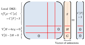
Figure 1: (Color online) Block structure of the linear system for the local solver. A few rows are also reserved for boundary conditions.

While it seems essential to represent the pitch-angle dependence of the potentials using Legendre polynomials, the distribution function itself need not be discretized in the same way, and there are many options available for the other coordinates, so a range of different discretization schemes were investigated. A choice of piecewise Chebyshev spectral colocation and finite-difference methods of various orders were implemented for both the $x$ and $\xi$ grids. The spectral colocation approach is highly accurate for given grid resolution. However, as the matrix is denser in the associated coordinate for these approaches, the solver slows more rapidly compared to finite differencing as the grid resolution increases. Thus, for satisfactory numerical convergence, high-order finite-difference methods are often preferable in practice. For discretization in $\theta$, finite-difference methods of various orders and spectral colocation as well as a sine/cosine modal representation have been implemented. The modal approach is extremely efficient for the simple concentric circular flux surface model, in which case the matrix is sparse in $\theta$. However, for shaped geometry, the matrix becomes dense in $\theta$ for the modal approach, so the colocation approach is both more convenient and similarly accurate. In shaped geometry, despite the accuracy of the spectral approaches, finite-difference differentiation again typically gives satisfactory convergence in less time due to the sparsity of the matrix.

The linear system may be solved using a sparse direct algorithm; a Krylov-space iterative solver may be much faster, but convergence of the algorithm then requires an effective preconditioner. One successful preconditioner is obtained by eliminating the off-diagonal blocks in Fig. 1 as well as the off-diagonal-in-$x$ terms in the energy scattering operator and boundary conditions. If high-order finite difference derivatives are used in $x$, convergence typically also requires that a constant $\sim\nu_{\mathrm{ii}}$ be added to the diagonal of the kinetic equation. We find the generalized minimum residual method (GMRES) does not converge consistently, while the stabilized biconjugate gradient and transpose-free quasi-minimal residual methods are more reliable.

Several issues regarding null solutions and symmetry properties of the distribution function are discussed in Appendix A.

Figures 2 and 3 show typical results of the local code, plotting the flow and thermal conductivity coefficients $k_{||}$ and $k_{q}$ as functions of aspect ratio and collisionality. Although the code can use general shaped geometry, for all plots in this paper we use the standard concentric circular flux surface model $B\propto 1/(1+\epsilon\cos\theta)$ and $\mbox{\boldmath$b$}\cdot\nabla\theta$ = constant, to facilitate comparison with previous literature on neoclassical theory. We may then take the definition of the ion collisionality to be $\nu_{*}=\nu_{\mathrm{ii}}/(\epsilon^{3/2}v_{\mathrm{i}}\nabla_{||}\theta)$.

Several approximate analytic formulae are also plotted. The Chang-Hinton formula for the heat fluxChang C S and Hinton F L (1982)

$$k_{q}=\frac{0.66+1.88\epsilon^{1/2}-1.54\epsilon}{1+1.03\nu_{*}^{1/2}+0.31\nu_{*}}\left<B^{2}\right>\left<\frac{1}{B^{2}}\right>+\frac{0.58\nu_{*}\epsilon}{1+0.74\nu_{*}\epsilon^{3/2}}\left(\left<B^{2}\right>\left<\frac{1}{B^{2}}\right>-1\right)$$ (14)

and the formula of Sauter et alSauter O, Angioni C, and Lin-Liu Y R (1999)

$$k_{||}=-\left[\frac{1}{1+0.5\sqrt{\nu_{*}}}\left(\frac{-1.17f_{\mathrm{c}}}{1-0.22f_{\mathrm{t}}-0.19f_{\mathrm{t}}^{2}}+0.25(1-f_{\mathrm{t}}^{2})\sqrt{\nu_{*}}\right)+0.315\nu_{*}^{2}f_{\mathrm{t}}^{6}\right]\frac{1}{1+0.15\nu_{*}^{2}f_{\mathrm{t}}^{6}}$$ (15)

apply to arbitrary aspect ratio, plasma shaping, and collisionality. (Note $\alpha$ in Ref. Sauter O, Angioni C, and Lin-Liu Y R, 1999 equals $-k_{||}$ in our notation.) Taguchi’s formula for the heat fluxTaguchi M (1988)

$$k_{q}=\frac{1}{\sqrt{\epsilon}}\left[\left<B^{2}\right>\left<\frac{1}{B^{2}}\right>-\frac{f_{\mathrm{c}}}{f_{\mathrm{c}}+0.462f_{\mathrm{t}}}\right],$$ (16)

and a formula for the flow coefficient derived on p.216 of Ref. Helander P and Sigmar D J, 2002

$$k_{||}=1.17f_{\mathrm{c}}/\left(f_{\mathrm{c}}+0.462f_{\mathrm{t}}\right).$$ (17)

are applicable at arbitrary aspect ratio and shaping in the limit of small $\nu_{*}$. An expression equivalent to the latter result was also given previously in Eq. (28) of Ref. Ernst D R, Bell M G, Bell R E, Bush C E, Chang Z, Fredrickson E, Grisham L R, Hill K W, Jassby D L, Mansfield D K, McCune D C, Park H K, Ramsey A T, Scott D S, Strachan J D, Synakowski E J, Taylor G, Thompson M and Weiland R M, 1998. (There, $\alpha_{2}=0.6562\sqrt{\epsilon}$ and $\alpha_{1}=1.173$. Taking $f_{\mathrm{t}}=1.46\sqrt{\epsilon}$ for circular flux surfaces yields the same result as (17).) Here, $f_{\mathrm{t}}=1-f_{\mathrm{c}}$ and

$$f_{\mathrm{c}}=\frac{3}{4}\left<B^{2}\right>\int_{0}^{1/B_{\mathrm{max}}}\frac{\lambda\;d\lambda}{\sqrt{1-\lambda B}}.$$ (18)

As Figure 2 shows, (17) does a reasonable job of predicting the low-collisionality limit of $k_{||}$. The analytic result $k_{||}=1.17$ obtained using a momentum-conserving pitch-angle scattering model collision operator is indeed the limiting value for $\nu_{*}\to 0$ and $\epsilon\to 0$ as expected, but $\epsilon$ must be $<0.01$ for this value to be a good approximation. Figure 3 shows Taguchi’s formula (16) is extremely accurate. The Chang-Hinton formula (14) is less accurate but it correctly captures the trends with $\epsilon$ and $\nu_{*}$.

Figure 2: (Color online) The flow coefficient $k_{||}$ defined in (6) for concentric circular flux surface geometry, as computed by the local code (solid) and the Sauter et al formula (15) (dashed). Squares show the Helander-Sigmar formula (17), an approximate analytical treatment of the $\nu_{*}\to 0$ limit, for the same four values of $\epsilon$. The arrow indicates the known analytic $\nu_{*}\to 0$, $\epsilon\to 0$ limit 1.17.

Figure 3: (Color online) The thermal conductivity coefficient $k_{q}$ defined in (5) for concentric circular flux surface geometry. Solid curves are computed by the local code. Dashed lines indicate the Chang-Hinton formula (14) for the same four values of $\epsilon$. Squares show the Taguchi formula (16), an approximate analytical treatment of the $\nu_{*}\to 0$ limit, again for the same four $\epsilon$. The arrow indicates the known analytic $\nu_{*}\to 0$, $\epsilon\to 0$ limit 0.66.

The local code was also compared with published results from the Fokker-Planck code of Ref. Wong S K and Chan V S, 2011; the remarkable agreement of the codes is shown in Figure 4.

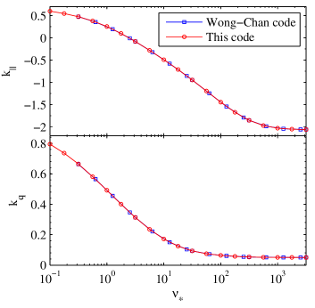
Figure 4: (Color online) The local code agrees to high precision with the Fokker-Planck code of Ref. Wong S K and Chan V S, 2011 for both the flow (a) and heat flux (b) coefficients. Calculations are shown for $\epsilon=0.1$. Data reproduced with permission.

Another set of transport coefficients arise in the analysis of the electrons. The radial particle and electron heat diffusivity are $\sim\sqrt{m_{\mathrm{e}}/m_{\mathrm{i}}}$ smaller than the ion heat transport and are always dominated by turbulent transport in practice, so we will not discuss them further. Of greater interest are the electrical conductivity and bootstrap current; these quantities are discussed in Section VI.

The distribution function obtained by the local solver has several noteworthy features. In the $\nu_{*}\ll 1$ limit, analysis shows the $g$ piece of the distribution function should vanish in the trapped region of phase spaceHinton F L and Hazeltine R D (1976); Helander P and Sigmar D J (2002), and a boundary layer exists between the trapped and passing regionsHinton F L and Rosenbluth M N (1973). These properties are reproduced in the code, as illustrated in Figure 5. The thickness of this boundary layer increases with collisionality. Although the collisionality $\nu_{*}$ is typically defined in terms of the thermal speed $v_{\mathrm{i}}$, each value of $v$ in phase space effectively has its own collisionality given by $~{}\nu_{\mathrm{D}}/(v\epsilon^{3/2}\mbox{\boldmath$b$}\cdot\nabla\theta)$, with faster particles being less collisional. As shown in the figure, the boundary layer indeed grows narrower with $v$. In Figure 5.c, $g$ at each $v$ is scaled to go to 1 at $\xi=1$ for clarity. Also notice in Figure 5.a-b that $g$ is nearly constant along particle trajectories, as it should be.

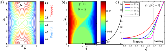
Figure 5: (Color online) a) Particle orbits, i.e contours of magnetic moment $\mu$, for $\epsilon=0.3$. b) The “collisional response” distribution $g$ at $v=v_{\mathrm{i}}$ for $\nu_{*}=0.01$, showing $g\approx 0$ for the trapped region as predicted by banana-regime analytic theory. c) A slice of $g$ at $\theta=0$ shows the boundary layer, which is narrower at larger $v$ due to the lower effective collisionality.

IV Global kinetic equation

Under what circumstances does the ion distribution remain close to a Maxwellian flux function, i.e., is the approximation $f_{\mathrm{i}}\approx f_{\mathrm{Mi}}(\psi)$ of section II valid? The magnitude of the correction to the flux-function Maxwellian may be estimated from the local theory roughly as $f_{1}\sim F\sim(\rho_{\theta}/r_{\bot})f_{\mathrm{Mi}}$ where $r_{\bot}$ is the scale length of variation in density and/or temperature. In a pedestal, since $\rho_{\theta}/r_{\bot}\sim 1$, then $f_{1}\sim f_{\mathrm{Mi}}$ and the neoclassical expansion breaks down.

However, a more careful estimate reveals there is a regime in which the near-Maxwellian assumption is still validKagan G and Catto P J (2010b). To define this regime, first write $f_{\mathrm{Mi}}$ in an equivalent form:

$$f_{\mathrm{Mi}}=\eta(\psi)\left[\frac{m_{\mathrm{i}}}{2\pi T_{\mathrm{i}}(\psi)}\right]^{3/2}\exp\left(-\frac{W_{0}}{T_{\mathrm{i}}(\psi)}\right)$$ (19)

where

$$\eta(\psi)=n_{\mathrm{i}}(\psi)\exp\left(Ze\Phi_{0}(\psi)/T_{\mathrm{i}}(\psi)\right)$$ (20)

and again $W_{0}=m_{\mathrm{i}}v^{2}/2+Ze\Phi_{0}$ is the leading-order total energy. Then the derivative $\partial f_{\mathrm{Mi}}/\partial\psi$ (at fixed $W_{0}$) that determines the magnitude of $f_{1}$ is

$$\frac{\partial f_{\mathrm{Mi}}}{\partial\psi}=\left[\frac{1}{\eta}\frac{d\eta}{d\psi}+\left(W_{0}-\frac{3}{2}\right)\frac{1}{T_{\mathrm{i}}}\frac{dT_{\mathrm{i}}}{d\psi}\right]f_{\mathrm{Mi}}$$ (21)

(equivalent to (2).) In this form, it is apparent that the magnitude of $\partial f_{\mathrm{Mi}}/\partial\psi$ is determined by $r_{T}$ and $r_{\eta}$, the scale-lengths of $T_{\mathrm{i}}$ and $\eta$, but not directly by $r_{n}$, the scale-length of density. Therefore $f_{1}/f_{\mathrm{Mi}}$ may be small compared to unity even when $r_{n}\sim\rho_{\theta}$ as long as $r_{T}$ and $r_{\eta}$ are $\gg\rho_{\theta}$.

This “weak-$T_{\mathrm{i}}^{\prime}$ pedestal” regime is the orderingKagan G and Catto P J (2008); Kagan G and Catto P J (2010b) we shall consider for the rest of the analysis: $\delta\ll 1$ where $\delta=\rho_{\theta}/r_{T}$, $\rho_{\theta}/r_{\eta}\sim\delta$, and $\rho_{\theta}/r_{n}\sim 1$. This regime is useful for two reasons: the collision operator may be linearized, and, as we will show, the poloidal electric field may be decoupled from the kinetic equation, eliminating the $\mbox{\boldmath$E$}\times\mbox{\boldmath$B$}$ nonlinearity. Therefore the kinetic equation is linear in $f_{1}$. For $r_{T}\sim\rho_{\theta}$ and/or $r_{\eta}\sim\rho_{\theta}$, a full-$f$ nonlinear kinetic equation must be solved, retaining both the collisional and $\mbox{\boldmath$E$}\times\mbox{\boldmath$B$}$ nonlinearities. Notice $r_{\eta}\ll 1$ implies the ions are electrostatically confined ($d\Phi_{0}/d\psi\approx-[Zen_{\mathrm{i}}]^{-1}dp_{\mathrm{i}}/d\psi$) with $(Ze/T_{\mathrm{i}})d\Phi_{0}/d\psi\sim 1/(RB_{\theta}\rho_{\theta})$, so $Ze\Phi_{0}/T_{\mathrm{i}}\sim 1$. Due to this ordering for the electric field, the $\mbox{\boldmath$v$}_{E}\cdot\nabla f_{\mathrm{i}}$ term in the kinetic equation, neglected in conventional neoclassical calculations, becomes comparable to the $v_{||}\nabla_{||}f_{\mathrm{i}}$ streaming term. Therefore, although $f_{1}\ll f_{\mathrm{Mi}}$ in the weak-$T_{\mathrm{i}}^{\prime}$ pedestal, conventional neoclassical results must still be modified.

Now, consider the full-$f$ drift-kinetic equationHazeltine R D (1973)

$$v_{||}\nabla_{||}f_{\mathrm{i}}+\mbox{\boldmath$v$}_{\mathrm{d}}\cdot\nabla f_{\mathrm{i}}=C_{\mathrm{nl}}\{f_{\mathrm{i}}\}+S$$ (22)

where $S$ represents any sources/sinks and $C_{\mathrm{nl}}$ is the nonlinear Fokker-Planck-Landau operator. As pointed out by HazeltineHazeltine R D (1973), (22) may be derived recursively, and so its validity does not require $|v_{||}\nabla_{||}f_{\mathrm{i}}|\gg|\mbox{\boldmath$v$}_{\mathrm{d}}\cdot\nabla f_{\mathrm{i}}|$. Since $f_{\mathrm{i}}\approx f_{\mathrm{Mi}}$ to leading order, $C_{\mathrm{nl}}$ may be approximated with $C_{\mathrm{i}}$, the operator linearized about $f_{\mathrm{Mi}}$. For the drift velocity $\mbox{\boldmath$v$}_{\mathrm{d}}$ it will be convenient to use $\mbox{\boldmath$v$}_{\mathrm{d}}=(v_{||}/\Omega)\nabla\times(v_{||}\mbox{\boldmath$b$})$ (discussed in appendix B) where the gradient acts at fixed $\mu$ and $W$. We make the ansatz $\Phi_{1}\sim\delta\;\Phi_{0}$ and $\partial\Phi_{1}/\partial\psi\sim\delta\;d\Phi_{0}/d\psi$, and we will show shortly that these assumptions are self-consistent. We define $f_{1}$ by $f_{\mathrm{i}}=f_{\mathrm{Mi}}-(Ze\Phi_{1}/T_{\mathrm{i}})f_{\mathrm{Mi}}+f_{1}$, and change the independent variable from $W$ to $W_{0}$. Neglecting several $\Phi_{1}$ terms that are small in $\delta$,

$$\left(v_{||}\mbox{\boldmath$b$}+\mbox{\boldmath$v$}_{\mathrm{d}}\right)\cdot\nabla f_{1}-C_{\mathrm{i}}\{f_{1}\}=-\mbox{\boldmath$v$}_{\mathrm{d}}\cdot\nabla\psi\frac{\partial f_{\mathrm{Mi}}}{\partial\psi}+S.$$ (23)

The contribution from $\Phi_{1}$ to $\mbox{\boldmath$v$}_{\mathrm{d}}\cdot\nabla\theta$ is $O(\delta)$ smaller than the $\Phi_{0}$ contribution, and $(\mbox{\boldmath$v$}_{E}\cdot\nabla\psi)/(\mbox{\boldmath$v$}_{\mathrm{m}}\cdot\nabla\psi)\sim Ze\Phi_{1}/T_{\mathrm{i}}\sim\delta$ where $\mbox{\boldmath$v$}_{\mathrm{m}}=\mbox{\boldmath$v$}_{\mathrm{d}}-\mbox{\boldmath$v$}_{E}$ is the magnetic drift, so $\Phi_{1}$ may be entirely neglected in $\mbox{\boldmath$v$}_{\mathrm{d}}$ and (23). We therefore approximate $\mbox{\boldmath$v$}_{\mathrm{d}}$ in (23) with $\mbox{\boldmath$v$}_{\mathrm{d0}}=\mbox{\boldmath$v$}_{\mathrm{m}}+\mbox{\boldmath$v$}_{E0}$ where $\mbox{\boldmath$v$}_{E0}=cB^{-2}\mbox{\boldmath$B$}\times\nabla\Phi_{0}$. To evaluate $\Phi_{1}$ we may use the adiabatic electron density response $n_{\mathrm{e}}+(e\Phi_{1}/T_{\mathrm{e}})n_{\mathrm{e}}$, where $n_{\mathrm{e}}(\psi)=Zn_{\mathrm{i}}(\psi)$ is the leading-order electron density, with quasineutrality to obtain

$$e\Phi_{1}/T_{\mathrm{i}}=\left(T_{\mathrm{i}}/T_{\mathrm{e}}+Z\right)^{-1}n_{\mathrm{i}}^{-1}\int d^{3}v\,f_{1}.$$ (24)

Hence, as $f_{1}\sim\delta f_{\mathrm{Mi}}$, the ordering ansatz for $\Phi_{1}$ above is self-consistent. As both the collisional and $\mbox{\boldmath$E$}\times\mbox{\boldmath$B$}$ nonlinearities are thus formally negligible, (23) is completely linear.

Just as in the local case, it is convenient to define the collisional response part of the distribution function $g$ using (4). Eliminating $f_{1}$ in (23) in favor of $g$, a pair of terms cancels. We also drop the resulting $\mbox{\boldmath$v$}_{\mathrm{d0}}\cdot\nabla\left[(Iv_{||}/\Omega)\partial f_{\mathrm{Mi}}/\partial\psi\right]$ term because $\mbox{\boldmath$v$}_{\mathrm{d0}}\cdot\nabla(Iv_{||}/B)\propto\nabla\times[(v_{||}/B)\mbox{\boldmath$B$}]\cdot\nabla(Iv_{||}/B)=0$ exactly and $\mbox{\boldmath$v$}_{\mathrm{d0}}\cdot\nabla(\partial f_{\mathrm{Mi}}/\partial\psi)$ is small in $\delta$. Thus, we obtain

$$\left(v_{||}\mbox{\boldmath$b$}+\mbox{\boldmath$v$}_{\mathrm{d0}}\right)\cdot\nabla g-C_{\mathrm{i}}\{g\}=C_{\mathrm{i}}\{F\}+S.$$ (25)

The advantage of this second form is that it makes clear that gradients in $n_{\mathrm{i}}$, $\Phi_{0}$, and/or $\eta$ cannot affect the $g$ part of the distribution function – only a $T_{\mathrm{i}}$ gradient can drive $g$. The logic is the same as in the local case: $C_{\mathrm{i}}\{v_{||}f_{\mathrm{Mi}}\}=0$, so the only gradient surviving in the inhomogeneous drive term (13) is $dT_{\mathrm{i}}/d\psi$. This property is obscured in the form (23). While the independence of $g$ from $dn_{\mathrm{i}}/d\psi$ and $d\Phi_{0}/d\psi$ was well known previously for the local case, it is noteworthy that this property persists in the weak-$T_{\mathrm{i}}^{\prime}$ pedestal case considered hereKagan G and Catto P J (2010b).

V Changes to flow structure

Two noteworthy differences between the local and global analyses are that the parallel flow coefficient $k_{||}$, as defined in (6), no longer needs to be constant on a flux surface, and it no longer also describes the poloidal flow. To see the first of these points, we may apply the operation $\int d^{3}v$ to the kinetic equation (25), as detailed in appendix B. The resulting mass conservation equation (ignoring sources) is

$$\nabla\cdot\left(\int d^{3}v(v_{||}\mbox{\boldmath$b$}+\mbox{\boldmath$v$}_{E0}+\mbox{\boldmath$v$}_{\mathrm{m}})g\right)=0.$$ (26)

Recall from section II that in the local case, the $v_{||}$ term in (26) dominates the others, implying $\int d^{3}v\,v_{||}g\propto B$. This result was crucial for proving the constancy of $k_{||}$ on a flux surface, for the $dT_{\mathrm{i}}/d\psi$ term in the parallel flow is precisely $\int d^{3}v\,v_{||}g$. However, in the global case, (26) indicates that $\int d^{3}v\,v_{||}g$ need not vary on a flux surface in proportion to $B$, so the proof for the constancy of $k_{||}$ breaks down.

These same results can be derived from a fluid perspective, making no reference to the drift-kinetic equation, starting instead from the fluid mass flow

$$\mbox{\boldmath$\Gamma$}=\int d^{3}v\left(v_{||}\mbox{\boldmath$b$}+\mbox{\boldmath$v$}_{E}+\mbox{\boldmath$v$}_{\mathrm{m}}\right)f_{\mathrm{i}}-\nabla\times\mbox{\boldmath$M$}$$ (27)

where $\mbox{\boldmath$M$}=\mbox{\boldmath$b$}\int d^{3}vf_{\mathrm{i}}v_{\bot}^{2}/\Omega$. Equivalently,

$$\mbox{\boldmath$\Gamma$}=\Gamma_{||}\mbox{\boldmath$b$}+\mbox{\boldmath$\Gamma$}_{E}+\mbox{\boldmath$\Gamma$}_{\mathrm{dia}},$$ (28)

where $\mbox{\boldmath$\Gamma_{E}$}=\int d^{3}v\,f_{\mathrm{i}}\mbox{\boldmath$v$}_{E}$, $\mbox{\boldmath$\Gamma$}_{\mathrm{dia}}=c(ZeB^{2})^{-1}\mbox{\boldmath$B$}\times\nabla\cdot\mbox{\boldmath$\overleftrightarrow{\Pi}$}$ is the diamagnetic flow, $\mbox{\boldmath$\overleftrightarrow{\Pi}$}=p_{\bot}(\mbox{\boldmath$\overleftrightarrow{I}$}-\mbox{\boldmath$b$}\mbox{\boldmath$b$})+p_{||}\mbox{\boldmath$b$}\mbox{\boldmath$b$}$, $p_{\bot}=m_{\mathrm{i}}\int d^{3}v\,f_{\mathrm{i}}v_{\bot}^{2}/2$, and $p_{||}=m_{\mathrm{i}}\int d^{3}v\,f_{\mathrm{i}}v_{||}^{2}$. The equivalence of (27) and (28) follows from

$$\int d^{3}v\,f_{\mathrm{i}}\mbox{\boldmath$v$}_{\mathrm{m}}-\nabla\times\mbox{\boldmath$M$}=\mbox{\boldmath$\Gamma$}_{\mathrm{dia}},$$ (29)

which may be derivedHinton F L and Hazeltine R D (1976) using the more accurate drift $\mbox{\boldmath$v$}_{\mathrm{m}}=v_{||}^{2}\Omega^{-1}\mbox{\boldmath$b$}\times\mbox{\boldmath$\kappa$}+v_{\bot}^{2}(2\Omega B)^{-1}\mbox{\boldmath$b$}\times\nabla B+v_{\bot}^{2}(2\Omega B)^{-1}\mbox{\boldmath$b$}\mbox{\boldmath$b$}\cdot\nabla\times\mbox{\boldmath$b$}$. (This drift is identical to our earlier expression to leading order in $\beta\ll 1$.) Notice $\mbox{\boldmath$b$}\cdot$(28) with (4) and $V_{||}=\mbox{\boldmath$\Gamma$}\cdot\mbox{\boldmath$b$}/n_{\mathrm{i}}$ gives (6) with $k_{||}=Ze\left<B^{2}\right>(cIn_{\mathrm{i}}B\,dT_{\mathrm{i}}/d\psi)^{-1}\int d^{3}v\,v_{||}v$ as before.

We now impose mass conservation $\nabla\cdot\mbox{\boldmath$\Gamma$}=0$, substituting (4) into (27), applying $\mbox{\boldmath$B$}\times\nabla\psi=I\mbox{\boldmath$B$}-R^{2}B^{2}\nabla\zeta$, and noting $\int d^{3}v\;\mbox{\boldmath$v$}_{\mathrm{m}}f_{\mathrm{Mi}}=c(ZeB^{2})^{-1}(dp_{\mathrm{i}}/d\psi)\mbox{\boldmath$B$}\times\nabla\psi+\nabla\times[cp_{\mathrm{i}}\mbox{\boldmath$b$}/(ZeB)]$. Cancellations occur to leave $T_{1}+T_{2}+T_{3}+T_{4}=0$ where $T_{1}=\nabla\cdot\int d^{3}v(v_{||}\mbox{\boldmath$b$}+\mbox{\boldmath$v$}_{E0}+\mbox{\boldmath$v$}_{\mathrm{m}})g$, $T_{2}=-\nabla\cdot\int d^{3}v(\mbox{\boldmath$v$}_{E0}+\mbox{\boldmath$v$}_{\mathrm{m}})Ze\Phi_{1}f_{\mathrm{Mi}}/T_{\mathrm{i}}$, $T_{3}=\nabla\cdot\int d^{3}v\,\mbox{\boldmath$v$}_{E1}f_{\mathrm{Mi}}=\nabla\cdot(cn_{\mathrm{i}}B^{-2}\mbox{\boldmath$B$}\times\nabla\Phi_{1})$, and $T_{4}=\nabla\cdot\int d^{3}v\;\mbox{\boldmath$v$}_{E1}(-ZeT_{\mathrm{i}}^{-1}f_{\mathrm{Mi}}\Phi_{1}+F+g)$ where $\mbox{\boldmath$v$}_{E1}=cB^{-2}\mbox{\boldmath$B$}\times\nabla\Phi_{1}$. As $\nabla n_{\mathrm{i}}=-(Zen_{\mathrm{i}}/T_{\mathrm{i}})\nabla\Phi_{0}+O(\delta)$ in our ordering, $T_{2}$ and $T_{3}$ cancel to leading order in $\delta$. It can be verified that the terms in $T_{4}$ are $O(\delta)$ smaller than the terms in $T_{1}$, so to leading order, $T_{1}=0$, which is precisely (26), but re-derived from a fluid rather than drift-kinetic perspective. The fluid analysis thereby confirms $k_{||}$ is no longer constant on each flux surface. Compared to the fluid analysis in the conventional ordering, reviewed following (9), it can be seen that two new contributions to mass conservation become important: $\mbox{\boldmath$E$}\times\mbox{\boldmath$B$}$ convection of the poloidally varying density, and radial variation of the particle flux or (equivalently) diamagnetic flow. Even though $|\mbox{\boldmath$v$}_{E0}|\ll v_{\mathrm{i}}$, $\mbox{\boldmath$E$}\times\mbox{\boldmath$B$}$ convection of the density carried by $g$ matters for mass conservation (26) because the parallel flow only enters multiplied by the small factor $B_{\theta}/B$. And although $\mbox{\boldmath$\overleftrightarrow{\Pi}$}\approx p_{\mathrm{i}}\mbox{\boldmath$\overleftrightarrow{I}$}$, the radial derivative in $\nabla\cdot\mbox{\boldmath$\Gamma$}$ means the next-order correction to $\overleftrightarrow{\Pi}$ in the diamagnetic flow (or equivalently the radial neoclassical flux) must be retained to accurately compute $\nabla\cdot\mbox{\boldmath$\Gamma$}$.

The poloidal fluid flow $V_{\theta}$ is found by computing $V_{\theta}=\mbox{\boldmath$\Gamma$}\cdot\mbox{\boldmath$e$}_{\theta}/n_{\mathrm{i}}$, using (27) or (28). Plugging (4) into $\mbox{\boldmath$e$}_{\theta}\cdot$(27), several cancelations occur, leaving

$$V_{\theta} = \underbrace{\frac{B_{\theta}}{Bn_{\mathrm{i}}}\int d^{3}v\,v_{||}g}_{V_{1}}+\underbrace{\frac{cIB_{\theta}}{B^{2}n_{\mathrm{i}}}\frac{d\Phi_{0}}{d\psi}\int d^{3}v\,g}_{V_{2}}-\underbrace{\frac{\mbox{\boldmath$e$}_{\theta}}{n_{\mathrm{i}}}\cdot\nabla\times\int d^{3}v\frac{v_{\bot}^{2}}{2\Omega}g\mbox{\boldmath$b$}}_{V_{3}}+\frac{\mbox{\boldmath$e$}_{\theta}}{n_{\mathrm{i}}}\cdot\int d^{3}v\,\mbox{\boldmath$v$}_{\mathrm{m}}g$$

$$-\frac{Ze\Phi_{1}}{T_{\mathrm{i}}}\frac{cIB_{\theta}}{B^{2}}\left[\frac{d\Phi_{0}}{d\psi}+\frac{T_{i}}{Zen_{\mathrm{i}}}\frac{dn_{\mathrm{i}}}{d\psi}\right]+\mbox{\boldmath$B$}\times\nabla\Phi_{1}\cdot\mbox{\boldmath$e$}_{\theta}\frac{c}{B}\left(-\frac{Ze\Phi_{1}}{T_{\mathrm{i}}}+\frac{1}{n_{\mathrm{i}}}\int d^{3}v\,g\right).$$

So far no terms have been dropped. We now order the terms using the orderings developed in Section IV. Using $(Ze/T_{\mathrm{i}})d\Phi_{0}/d\psi\sim 1/(RB_{\theta}\rho_{\theta})$ it can be verified that $V_{1}\sim V_{2}$. It can also be verified that each term following $V_{3}$ is $O(\delta)$ smaller than $V_{1}\sim V_{2}$ using $\int d^{3}v\,g\sim\delta n_{\mathrm{i}}$, $Ze\Phi_{1}/T_{\mathrm{i}}\sim\delta$, $\nabla\Phi_{1}\cdot\mbox{\boldmath$B$}\times\mbox{\boldmath$e$}_{\theta}\approx-IB_{\theta}\partial\Phi_{1}/\partial\psi\sim\delta IB_{\theta}d\Phi_{0}/d\psi$, and noting the quantities in square brackets cancel to leading order.

It remains to evaluate $V_{3}$. The leading order contribution comes from the radial gradient of the integral of $g$, since only this derivative has the short scale length $\rho_{\theta}$. Thus, we obtain

$$V_{\theta}\approx\frac{B_{\theta}}{n_{\mathrm{i}}B}\left[\int d^{3}v\left(v_{||}+\frac{cI}{B}\frac{d\Phi_{0}}{d\psi}\right)g+\frac{I}{\Omega}\frac{\partial}{\partial\psi}\int d^{3}v\frac{v_{\bot}^{2}}{2}g\right].$$ (31)

In the local case, only the $v_{||}$ term arose in the analogous integral for $V_{\theta}$. In the pedestal we may define a normalized poloidal flow

$$k_{\theta}=V_{\theta}Ze\left<B^{2}\right>/(cIB_{\theta}\,dT_{\mathrm{i}}/d\psi)$$ (32)

so $k_{\theta}\to k_{||}$ in the local limit. The property $V_{\theta}\propto dT_{\mathrm{i}}/d\psi$ from conventional theory persists in the pedestal, due to (31) and $g\propto dT_{\mathrm{i}}/d\psi$.

VI Electron kinetics and parallel current

The orbit width for electrons is $\sim\sqrt{m_{\mathrm{e}}/m_{\mathrm{i}}}$ thinner than that of the ions, so direct finite-orbit-width effects for electrons may be neglected. However, the electrons are affected by modifications to the main ion flow. To demonstrate this point, and to show applications of the local Fokker-Planck code to electron quantities, we now analyze the electron kinetics. Since the particle and electron heat transport are essentially always dominated by turbulent transport, we focus here instead on the neoclassical conductivity and bootstrap current. Though the analysis below uses the pedestal ordering, conventional results for the parallel current are exactly recovered in the appropriate limit of the expressions derived here.

Using the gauge of Appendix C, the electron kinetic equation may be written

$$(v_{||}\mbox{\boldmath$b$}+\mbox{\boldmath$v$}_{\mathrm{me}}+\mbox{\boldmath$v$}_{E})\cdot(\nabla f_{\mathrm{e}})_{w}-ev_{||}\left<E_{||}B\right>B\left<B^{2}\right>^{-1}\partial f_{\mathrm{e}}/\partial w=C_{\mathrm{e}}$$ (33)

where $\mbox{\boldmath$v$}_{\mathrm{me}}$ is the electron magnetic drift, $w=m_{\mathrm{e}}v^{2}/2-e\Phi$ is an independent variable, and $C_{\mathrm{e}}$ is the total electron collision operator. We assume $f_{\mathrm{e}}\approx f_{\mathrm{Me}}$ where

$$f_{\mathrm{Me}}=n_{\mathrm{e}}(\psi)\left[\frac{m_{\mathrm{e}}}{2\pi T_{\mathrm{e}}(\psi)}\right]^{3/2}\exp\left(\frac{m_{\mathrm{e}}v^{2}}{2T_{\mathrm{e}}(\psi)}\right).$$ (34)

Then $C_{\mathrm{e}}=C_{\mathrm{ee}}+C_{\mathrm{ei}}$ where $C_{\mathrm{ee}}$ is equivalent to (11) but with ion quantities replaced by electron quantities, $C_{\mathrm{ei}}\{f_{\mathrm{e1}}\}\approx\nu_{\mathrm{ei}}L\{f_{\mathrm{e1}}\}+f_{\mathrm{Me}}\nu_{\mathrm{ei}}m_{\mathrm{e}}v_{||}V_{\mathrm{i}||}/T_{\mathrm{e}}$, $\nu_{\mathrm{ei}}=3\sqrt{\pi}/(4\tau_{\mathrm{ei}}x^{3})$, $x=v/v_{\mathrm{e}}$, $v_{\mathrm{e}}=\sqrt{2T_{\mathrm{e}}/m_{\mathrm{e}}}$, and $\tau_{\mathrm{ei}}=3\sqrt{m_{\mathrm{e}}}T_{\mathrm{e}}^{3/2}/(4\sqrt{2\pi}n_{\mathrm{e}}Ze^{4}\ln\Lambda)$. We write $f_{\mathrm{e}}=f_{\mathrm{Me}}\exp(e\Phi_{1}/T_{\mathrm{e}})+m_{\mathrm{e}}v_{||}V_{||}f_{\mathrm{Me}}/T_{\mathrm{e}}+h$ and solve for $h$. We also make a change of independent variables in the kinetic equation to $w_{0}=m_{\mathrm{e}}v^{2}/2-e\Phi_{0}$. Using (6), the leading terms in $\delta$ and $\sqrt{m_{\mathrm{e}}/m_{\mathrm{i}}}$ are

$$v_{||}\nabla_{||}h_{0}+\mbox{\boldmath$v$}_{\mathrm{me}}\cdot\nabla f_{\mathrm{Me}}+f_{\mathrm{Me}}\left(\frac{1}{p_{\mathrm{e}}}\frac{dp_{\mathrm{i}}}{d\psi}+\frac{e}{T_{\mathrm{e}}}\frac{d\Phi_{0}}{d\psi}\right)v_{||}\nabla_{||}\left(\frac{Iv_{||}}{\Omega_{\mathrm{e}}}\right)=C_{\mathrm{ee}}\{h_{0}\}+\nu_{\mathrm{ei}}L\{h_{0}\}$$ (35)

where $\Omega_{\mathrm{e}}=-eB/(m_{\mathrm{e}}c)$, $h_{0}$ is the first term in a series $h=h_{0}+h_{1}+\ldots$, and the inductive term has been taken as higher order. The solution to (35) may be written $h_{0}=cIe^{-1}(h_{p}\,dp/d\psi+h_{T_{\mathrm{e}}}n_{\mathrm{e}}dT_{\mathrm{e}}/d\psi)$ where $p=p_{\mathrm{e}}+p_{\mathrm{i}}$, and $h_{p}$ and $h_{T_{\mathrm{e}}}$ are the solutions to

$$D_{\mathrm{e}}h_{p} = -f_{\mathrm{Me}}n_{\mathrm{e}}^{-1}x^{2}(1+\xi^{2})B^{-2}\nabla_{||}B,$$ (36)

$$D_{\mathrm{e}}h_{T_{\mathrm{e}}} = -f_{\mathrm{Me}}n_{\mathrm{e}}^{-1}x^{2}(x^{2}-5/2)(1+\xi^{2})B^{-2}\nabla_{||}B,$$ (37)

with $D_{\mathrm{e}}=v_{||}\nabla_{||}-C_{\mathrm{ee}}-\nu_{\mathrm{ei}}L$. Recalling $e\Phi_{1}/T_{\mathrm{i}}\sim\delta$, the $O(\delta)$ terms in the kinetic equation are

$$Dh_{1}-\frac{f_{\mathrm{Me}}I}{ZT_{\mathrm{e}}\left<B^{2}\right>}\frac{dT_{\mathrm{i}}}{d\psi}v_{||}\nabla_{||}\left(\frac{k_{||}v_{||}B^{2}}{\Omega_{\mathrm{e}}}\right)+\mbox{\boldmath$v$}_{E1}\cdot\nabla f_{\mathrm{Me}}+e\Phi_{1}\mbox{\boldmath$v$}_{\mathrm{me}}\cdot\nabla(f_{\mathrm{Me}}/T_{\mathrm{e}})$$

$$+ev_{||}(\nabla_{||}\Phi_{1})\frac{\partial h_{0}}{\partial w_{0}}+\frac{ev_{||}\left<E_{||}B\right>B}{T_{\mathrm{e}}\left<B^{2}\right>}f_{\mathrm{Me}}=0$$ (38)

where $\mbox{\boldmath$v$}_{E1}=cB^{-2}\mbox{\boldmath$B$}\times\nabla\Phi_{1}$, and we have assumed $\sqrt{m_{\mathrm{e}}/m_{\mathrm{i}}}\ll\delta$. The solution may be written $h_{1}=-h_{E}e^{-1}\left<E_{||}B\right>-cIe^{-1}n_{\mathrm{i}}h_{T_{\mathrm{i}}}\,dT_{\mathrm{i}}/d\psi-\rho_{0}cI^{2}(dn_{\mathrm{e}}/d\psi)(dT_{\mathrm{i}}/d\psi)h_{\Phi}/e$ where $\rho_{0}=v_{\mathrm{i}}m_{\mathrm{i}}c/(ZeB_{\mathrm{av}})$, and $B_{\mathrm{av}}^{2}=\left<B^{2}\right>$. Here, $h_{E}$, $h_{T_{\mathrm{i}}}$, and $h_{\Phi}$ are the solutions of

$$D_{\mathrm{e}}h_{E} = f_{\mathrm{Me}}e^{2}T_{\mathrm{e}}^{-1}\left<B^{2}\right>^{-1}Bv_{||},$$ (39)

$$D_{\mathrm{e}}h_{T_{\mathrm{i}}} = f_{\mathrm{Me}}m_{\mathrm{e}}(n_{\mathrm{e}}T_{\mathrm{e}})^{-1}\left<B^{2}\right>^{-1}v_{||}\nabla_{||}\left(v_{||}Bk_{||}\right)$$ (40)

$$= f_{\mathrm{Me}}n_{\mathrm{e}}^{-1}x^{2}\left<B^{2}\right>^{-1}\left[k_{||}(3\xi^{2}-1)\nabla_{||}B-2\xi^{2}B\nabla_{||}k_{||}\right],$$

$$\frac{\rho_{0}cI^{2}}{e}\frac{dn_{\mathrm{e}}}{d\psi}\frac{dT_{\mathrm{i}}}{d\psi}Dh_{\Phi} = \mbox{\boldmath$v$}_{E1}\cdot\nabla f_{\mathrm{Me}}+e\Phi_{1}\mbox{\boldmath$v$}_{\mathrm{me}}\cdot\nabla\left(\frac{f_{\mathrm{Me}}}{T_{\mathrm{e}}}\right)+ev_{||}(\nabla_{||}\Phi_{1})\frac{\partial h_{0}}{\partial w_{0}}.$$ (41)

Note in the local case, $\nabla_{||}k_{||}=0$ so the last term in (40) vanishes and $h_{T_{\mathrm{i}}}\propto k_{||}$. The $D_{\mathrm{e}}$ operator, which is radially local in that $\psi$ is merely a parameter, may be inverted numerically for the right-hand sides (36)-(37) and (39)-(41) just as described in Section III for the similar ion operator $v_{||}\nabla_{||}-C_{\mathrm{ii}}$. Then the parallel current is

$$j_{||}=Zen_{\mathrm{i}}V_{\mathrm{i}||}-e\int d^{3}v\;f_{\mathrm{e}}=-e\int d^{3}v\;v_{||}h.$$ (42)

Now consider the result of applying $\int d^{3}v=2\pi m_{\mathrm{i}}^{-1}\sum_{\sigma}\sigma\int_{0}^{\infty}dv\int_{0}^{v^{2}/(2B)}d\mu\,Bv/v_{||}$ to (39). This operation annihilates both the right-hand side and the collision operators in $D_{\mathrm{e}}$, leaving $(\partial/\partial\theta)\int d^{3}v\,v_{||}h_{E}/B=0$. Therefore the flow carried by $h_{E}$ is $\int d^{3}v\,v_{||}h_{E}=\alpha_{E}B$ for some flux function $\alpha_{E}$. The same logic applies to (37), so $\int d^{3}v\,v_{||}h_{T_{\mathrm{e}}}=\alpha_{T_{\mathrm{e}}}B$ for some flux function $\alpha_{T_{\mathrm{e}}}$. Applying $\int d^{3}v$ to (36), the right-hand side is not annihilated this time, and we instead find $\int d^{3}v\,v_{||}h_{p}=B^{-1}+\alpha_{p}B$ for some flux function $\alpha_{p}$. Lastly applying $\int d^{3}v$ to the first equation in (40) and to (41), we obtain $\int d^{3}v\,v_{||}h_{T_{\mathrm{i}}}=\alpha_{T_{\mathrm{i}}}B+k_{||}B/\left<B^{2}\right>$ and $\int d^{3}v\,v_{||}h_{\Phi}=\alpha_{\Phi}B-n_{g}/(ZB)$ where $\alpha_{T_{\mathrm{i}}}$ and $\alpha_{\Phi}$ are flux functions, $n_{g}=T_{\mathrm{i}}(\rho_{0}In_{\mathrm{i}}\,dT_{\mathrm{i}}/d\psi)^{-1}\int d^{3}v\,g$ is the $O(1)$ normalized density carried by $g$, and we have invoked (24). Thus, the $dT_{\mathrm{i}}/d\psi$ term in the parallel current varies poloidally $\propto B$ in the local case where $k_{||}$ is constant, but not in the global case where $k_{||}$ varies.

Putting the pieces together, the total parallel current is

$$j_{||}=-\frac{cI}{B}\frac{dp}{d\psi}+\frac{cIn_{\mathrm{e}}Bk_{||}}{Z\left<B^{2}\right>}\frac{dT_{\mathrm{i}}}{d\psi}-\frac{\rho_{0}cI^{2}n_{g}}{ZB}\frac{dn_{\mathrm{e}}}{d\psi}\frac{dT_{\mathrm{i}}}{d\psi}+\alpha B$$ (43)

where $\alpha$ is another flux function. Multiplying this equation by $B$, flux-surface averaging, and substituting the result back into (43), we obtain

$$j_{||}=\frac{cI}{B}\frac{dp}{d\psi}\left(\frac{B^{2}}{\left<B^{2}\right>}-1\right)+\frac{cIn_{\mathrm{e}}B}{Z\left<B^{2}\right>}\frac{dT_{\mathrm{i}}}{d\psi}\left(k_{||}-\frac{\left<B^{2}k_{||}\right>}{\left<B^{2}\right>}\right)$$

$$+\frac{\rho_{0}cI^{2}}{Z}\frac{dn_{\mathrm{e}}}{d\psi}\frac{dT_{\mathrm{i}}}{d\psi}\left(\frac{\left<n_{g}\right>B}{\left<B^{2}\right>}-\frac{n_{g}}{B}\right)+\frac{\left<j_{||}B\right>B}{\left<B^{2}\right>}.$$ (44)

The $dp/d\psi$ term is the standard Pfirsch-Schlüter current, and the $\left<j_{||}B\right>$ term is the Ohmic and bootstrap contribution. However, the $k_{||}$ and $n_{g}$ terms are new in the global case, vanishing in the local case where $k_{||}$ is constant and $|\nabla n_{\mathrm{e}}|\rho_{\theta}\ll 1$. We may write the Ohmic and bootstrap contribution as

$$\left<j_{||}B\right>=\sigma_{\mathrm{neo}}\left<E_{||}B\right>-cIp_{\mathrm{e}}\left(\frac{\mathcal{L}_{31}}{p_{\mathrm{e}}}\frac{dp}{d\psi}+\frac{\mathcal{L}_{32}}{T_{\mathrm{e}}}\frac{dT_{\mathrm{e}}}{d\psi}-\frac{\mathcal{L}_{T_{\mathrm{i}}}}{ZT_{\mathrm{e}}}\frac{dT_{\mathrm{i}}}{d\psi}-\frac{\mathcal{L}_{nT}\rho_{0}I}{n_{\mathrm{e}}T_{\mathrm{e}}}\frac{dn_{\mathrm{e}}}{d\psi}\frac{dT_{\mathrm{i}}}{d\psi}\right)$$ (45)

where $\sigma_{\mathrm{neo}}=\left<B\int d^{3}v\;v_{||}h_{E}\right>$, $\mathcal{L}_{31}=\left<B\int d^{3}v\;v_{||}h_{p}\right>$, $\mathcal{L}_{32}=\left<B\int d^{3}v\;v_{||}h_{T_{\mathrm{e}}}\right>$, $\mathcal{L}_{T_{\mathrm{i}}}=\left<B\int d^{3}v\;v_{||}h_{T_{\mathrm{i}}}\right>$, and $\mathcal{L}_{nT}=\left<B\int d^{3}v\;v_{||}h_{\Phi}\right>$. The $\mathcal{L}_{nT}$ term in (45) is new, becoming negligible in the conventional case. For the local case of constant $k_{||}$, where $\mathcal{L}_{T_{\mathrm{i}}}\propto k_{||}$, it is useful to define $\mathcal{L}_{34}=\mathcal{L}_{T_{\mathrm{i}}}/k_{||}$ so $\mathcal{L}_{34}$ is completely independent of all ion quantities except $Z$. The definitions of $\sigma_{\mathrm{neo}}$, $\mathcal{L}_{31}$, $\mathcal{L}_{32}$, and $\mathcal{L}_{34}$ here are consistent with Ref. Sauter O, Angioni C, and Lin-Liu Y R, 1999. Interestingly, the new $n_{g}$ terms in (44) and (43) and the new $\mathcal{L}_{nT}$ term in (45) are quadratic in the gradients.

Figure 6 shows these coefficients of the bootstrap current and the conductivity as calculated by our code for the local limit $k_{||}$=constant, using the circular flux surface model and $Z=1$. The conductivity has been normalized by the parallel Spitzer value. The analytic fits to numerical calculations of the coefficients by Sauter et al are plotted for comparisonSauter O, Angioni C, and Lin-Liu Y R (1999). The horizontal coordinate in these plots is $\nu_{*\mathrm{e}}=\nu_{\mathrm{ee}}/(\epsilon^{3/2}\sqrt{2T_{\mathrm{e}}/m_{\mathrm{e}}}\mbox{\boldmath$b$}\cdot\nabla\theta)$, which is $1/\sqrt{2}$ smaller than the $\nu_{*\mathrm{e}}$ defined in Ref. Sauter O, Angioni C, and Lin-Liu Y R, 1999. We find the Sauter expressions give an excellent fit to the coefficients in the banana regime, though there is some discrepancy at higher collisionality when $\epsilon>0.1$, the same pattern observed in Figure 2. The reason for the discrepancy is unclear, since the fundamental kinetic equations and collision operators we use to generate figures 2 and 6 are identical to those solved by CQLP, the code to which the Sauter expressions are fit. (CQLP uses an adjoint method whereas our results do not, though this difference should not affect the physical results.) We have verified the difference persists when D-shaped Miller equilibrium is used, and the code of Ref. Wong S K and Chan V S, 2011 produces identical coefficients to ours. As shown in figure 7, the difference between our coefficients and those of Ref. Sauter O, Angioni C, and Lin-Liu Y R, 1999 can lead us to predict a reduced total bootstrap current density in the pedestal for experimentally relevant plasma parameters when $\nu_{*\mathrm{e}}>1$. This difference is primarily due to our lower $\mathcal{L}_{31}$, which multiplies the large $dp/d\psi$ term. When $\nu_{*\mathrm{e}}<1$, our prediction for the total bootstrap current density becomes indistinguishable from that of Ref. Sauter O, Angioni C, and Lin-Liu Y R, 1999.

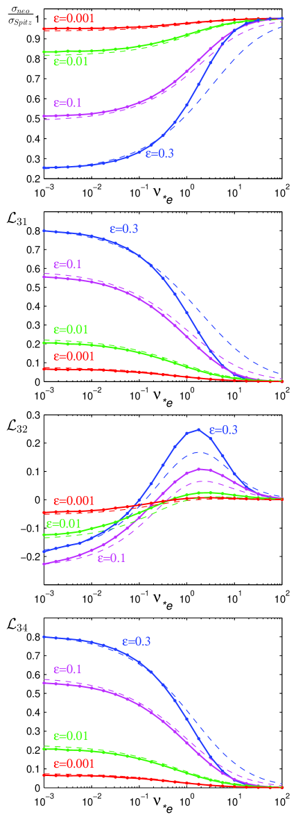
Figure 6: (Color online) Parallel current coefficients defined in (45) computed by our local code (dots, connected by solid curves). Dashed curves show the semi-analytic formulae of Sauter et alSauter O, Angioni C, and Lin-Liu Y R (1999).

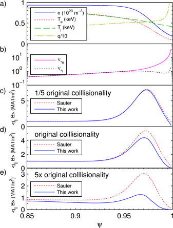
Figure 7: (Color online) a) Model profiles resembling the DIII-D measurements in figure (8) of Ref R. J. Groebner, T. H. Osborne, A. W. Leonard, and M. E. Fenstermacher1, 2009 and a plausible $q$ profile yield the collisionality profiles in b). c) The local code described here predicts identical total bootstrap current density to the formulae of Ref. Sauter O, Angioni C, and Lin-Liu Y R, 1999 for lower collisionality. d) We predict somewhat lower current density at the real collisionality, due primarily to the discrepancy in $\mathcal{L}_{31}$ shown in figure 6.b. e) At higher collisionalities, the differences become significant.

As with the flow, the total current vector $j$ remains divergence-free in the pedestal ordering:

$$0=\nabla\cdot\mbox{\boldmath$j$}=\nabla\cdot(j_{||}\mbox{\boldmath$b$}+cB^{-2}\mbox{\boldmath$B$}\times\nabla\cdot\mbox{\boldmath$\overleftrightarrow{\Pi}$}_{\Sigma})$$ (46)

where $\mbox{\boldmath$\overleftrightarrow{\Pi}$}_{\Sigma}=m\int d^{3}v\,\mbox{\boldmath$v$}\mbox{\boldmath$v$}(f_{\mathrm{i}}+f_{\mathrm{e}})$ is the total diagonal anisotropic stress, including $O(p)$ and $O(\delta p)$ terms. Equation (46) can be proved from (44) and (26) using (24), $f_{\mathrm{e}}\approx f_{\mathrm{Me}}+e\Phi_{1}f_{\mathrm{Me}}/T_{\mathrm{e}}$, and (29).) Equation (46) indicates the new $k_{||}$ and $n_{g}$ terms in (44) arise for the same fundamental reason as the conventional Pfirsch-Schlüter current: a parallel current must flow to maintain $\nabla\cdot\mbox{\boldmath$j$}=0$ given the perpendicular diamagnetic current. In the pedestal, the diamagnetic current associated with the poloidally varying pressure becomes large enough to modify the parallel current on the level of the $dT_{\mathrm{i}}/d\psi$ terms.

VII Global numerical scheme

It is equally valid and equally numerically challenging to solve either (23) or (25). For the rest of the analysis here we discuss the case of (25) for definiteness.

As we are interested in a narrow radial domain around the pedestal, we assume $I$, $B$, and $\nabla_{||}\theta$ are independent of $\psi$ for simplicity. These approximations are also convenient as they make $\mbox{\boldmath$v$}_{\mathrm{m}}\cdot\nabla\theta=0$ exactly for our form of the drifts. For simplicity, we also take $\eta$ and $T_{\mathrm{i}}$ to be constant over the simulation domain. The one place where $dT_{\mathrm{i}}/d\psi$ must be retained is in the inhomogeneous term, since the drive is $\propto dT_{\mathrm{i}}/d\psi$. As the kinetic equation is linear, $g$ may be normalized by $dT_{\mathrm{i}}/d\psi$, while every other appearance of $T_{\mathrm{i}}$ is treated as a constant.

Both versions of the global kinetic equation (23) and (25) resemble their local counterparts (1) and (3), but with the additional $\mbox{\boldmath$v$}_{\mathrm{d0}}\cdot\nabla$ term in the unknown. Due to the radial derivative in this term, the radial coordinate no longer enters the kinetic equation as a mere parameter, meaning the problem is now four-dimensional: $g=g(\psi,\theta,\mu,W_{0})$. In these original variables, the allowed range of each coordinate depends on the other coordinates in a complicated manner. For numerical work it is therefore convenient to change the independent variables from $(\mu,W_{0})$ to $(v,\xi)$ so the coordinate ranges become coordinate-independent. In these variables, the kinetic terms in (23) and (25) become

$$(v_{||}\mbox{\boldmath$b$}+\mbox{\boldmath$v$}_{\mathrm{d0}})\cdot(\nabla g)_{\mu,W_{0}}=K_{0}\{g\}+K_{E}\{g\}+\mbox{\boldmath$v$}_{\mathrm{m}}\cdot\nabla\psi\frac{\partial g}{\partial\psi}$$ (47)

where

$$K_{0}=v_{||}(\nabla_{||}\theta)\frac{\partial}{\partial\theta}-v\frac{(1-\xi^{2})}{2B}(\nabla_{||}B)\frac{\partial}{\partial\xi}$$ (48)

is the drift-kinetic operator implemented in conventional neoclassical codesBelli E A and Candy J (2008a); Wong S K and Chan V S (2011), and

$$K_{E}=\mbox{\boldmath$v$}_{E0}\cdot\nabla\theta\frac{\partial}{\partial\theta}+\xi cI\frac{d\Phi_{0}}{d\psi}\frac{(1-\xi^{2})}{2B^{2}}(\nabla_{||}B)\frac{\partial}{\partial\xi}-\mbox{\boldmath$v$}_{\mathrm{m}}\cdot\nabla\psi\frac{e}{m_{\mathrm{i}}v}\frac{d\Phi_{0}}{d\psi}\frac{\partial}{\partial v}$$ (49)

consists of new terms proportional to the radial electric field. In a pedestal, not only is the $\partial g/\partial\psi$ term in (47) important, but the terms in $K_{E}$ also become equally important. The aforementioned ordering for $d\Phi_{0}/d\psi$ implies each term in $K_{E}$ comparable in magnitude to $K_{0}$. Physically, the latter two terms in (49) are essential for maintaining conservation of $\mu$ and total energy as a particle’s kinetic energy changes during an orbit. This kinetic energy changes because the electrostatic potential seen by the particle varies over an orbit width.

We choose $n_{\mathrm{i}}(\psi)$, which determines $\Phi_{0}=(Ze)^{-1}T_{\mathrm{i}}\ln(\eta/n_{\mathrm{i}})$. On either end of the radial domain, we take $n_{\mathrm{i}}(\psi)$ and $\Phi_{0}(\psi)$ to be uniform for a distance of several $\rho_{\theta}$, as illustrated in figure 8.a-b. In this way, the distribution function will approximate the local neoclassical solution at the radial boundaries, so local solutions can be used there as inhomogeneous Dirichlet boundary conditions.

As the kinetic equation (25) is linear, it may in principle be solved numerically using a single matrix inversion. Indeed, this is the approach traditionally adopted by local neoclassical codes Belli E A and Candy J (2008a, b, 2009); Wong S K and Chan V S (2011), including the one described in Section III. However, this approach is already somewhat numerically challenging for the local problem due to the three-dimensional phase space, as the matrix has dimension $(N\theta\;Nv\;N\xi)\times(N\theta\;Nv\;N\xi)$, where $N\theta$, $Nv$, and $N\xi$ are the number of modes or grid points in the respective coordinates. In the nonlocal case, the additional spatial dimension means the matrix size must increase to $(N\psi\;N\theta\;Nv\;N\xi)\times(N\psi\;N\theta\;Nv\;N\xi)$ for $N\psi$ radial grid points, making such an approach much more time- and memory-intensive. Therefore we seek an alternative method.

In the new approach proposed here, a derivative with respect to a fictitious time $\partial g/\partial t$ is first added to the left-hand side of (25). For reasonable initial conditions and boundary conditions, $g$ should evolve towards an equilibrium since the equation (25) is dissipative. However, an explicit time-advance requires very small time steps for stability due to the many derivatives in the kinetic equation, and an implicit time-advance would require the inversion of a matrix just as large as for a direct solution of the original time-independent equation.

An effective solution is to employ the following operator-splitting technique. Consider the following series of two backwards-Euler time steps:

$$\frac{g_{t+(1/2)}-g_{t}}{\Delta t}+K_{\mathrm{NL}}\{g_{t+(1/2)}\} = 0,$$ (50)

$$\frac{g_{t+1}-g_{t+(1/2)}}{\Delta t}+K_{\mathrm{L}}\{g_{t+1}\} = C_{\mathrm{i}}\{F\}+S.$$ (51)

where $K_{\mathrm{L}}=K_{0}+K_{E}-C_{\mathrm{i}}$ is the “local operator” and $K_{\mathrm{NL}}=(\mbox{\boldmath$v$}_{\mathrm{m}}\cdot\nabla\psi)\partial/\partial\psi$ is the “nonlocal operator.” When summed together, $g_{t+(1/2)}$ cancels, leaving an equation that is equivalent to first order in $\Delta t$ to a backwards-Euler time step with the complete operator $K_{\mathrm{NL}}+K_{\mathrm{L}}$. However, each of the steps (50)-(51) are much easier than a step with the total operator because the dimensionality is reduced: e.g $\psi$ is only a parameter in (50), so this step requires the inversion of $N\psi$ matrices, each of size $(N\theta\;Nv\;N\xi)\times(N\theta\;Nv\;N\xi)$. Also notice that the local operator at each radial grid point need only be $LU$-factorized once, with the $L$ and $U$ factors reused at each time step for rapid implicit solves. The same is true of the nonlocal operator at each $v$ and $\xi$.

Several higher-order operator splitting schemes were explored, but none were found to be stable for the equation here.

The procedure outlined here provides a general recipe for extending a conventional neoclassical code into a pedestal code. A conventional neoclassical code inverts an operator $K_{0}-C_{\mathrm{i}}$, i.e. many of the terms in $K_{\mathrm{L}}$, so minor modifications would allow such a code to carry out the local part of the time advance. The modifications necessary are adding the electric field terms $K_{E}$ and adding the diagonal associated with the time derivative. The resulting operator is then iterated with the nonlocal operator.

For the results shown here we employ a piecewise-Chebyshev grid in $\psi$ with spectral colocation differentiation. A tiny artificial viscosity is required at the endpoints for numerical stability; the magnitude of this viscosity may be varied by many orders of magnitude with no perceptible change to the results. Inhomogeneous Dirichlet radial boundary conditions are imposed, with the distribution function at these points taken from the local code. For completeness, we have also tried upwinded high-order finite differences for radial differentiation, with the upwinding direction opposite above and below the midplane, corresponding to whether drift trajectories in the region move towards increasing or decreasing $\psi$. For our sign convention, the magnetic drifts are downward, so the inhomogeneous Dirichlet radial boundary condition must be specified above the midplane at large minor radius and below the midplane at small minor radius. This radial discretization scheme gives equivalent results to the Chebyshev method, but it requires more grid points for convergence, and a numerical instability tends to arise at large times.

VIII Need for a sink

In order to reach equilibrium, it is essential to include a heat sink. This requirement may be understood physically as follows. As we take the scale-lengths at each radial boundary to be large compared to $\rho_{\theta}$, the heat flux into the volume at small minor radius and the heat flux out of the volume at large minor radius are determined by the local neoclassical result (5). These fluxes are different due to the different densities at the two boundaries, and so net heat will constantly leave (or enter) the simulation domain. More rigorously, as shown in appendix B, the $\left<\int d^{3}v(\;\cdot\;)\right>$ and $\int_{\psi_{\mathrm{min}}}^{\psi_{\mathrm{max}}}d\psi\,V^{\prime}\left<\int d^{3}v(m_{\mathrm{i}}v^{2}/2)(\;\cdot\;)\right>$ moments of the kinetic equation in steady state give

$$\frac{1}{V^{\prime}}\frac{d}{d\psi}V^{\prime}\left<\int d^{3}v\,g\mbox{\boldmath$v$}_{\mathrm{m}}\cdot\nabla\psi\right>=\left<\int d^{3}v\,S\right>,$$ (52)

$$\left[V^{\prime}\left<\int d^{3}v\,g\frac{m_{\mathrm{i}}v^{2}}{2}\mbox{\boldmath$v$}_{\mathrm{m}}\cdot\nabla\psi\right>\right]_{\psi_{\mathrm{min}}}^{\psi_{\mathrm{max}}}+Ze\int_{\psi_{\mathrm{min}}}^{\psi_{\mathrm{max}}}d\psi\,V^{\prime}\frac{d\Phi_{0}}{d\psi}\left<\int d^{3}v\,g\mbox{\boldmath$v$}_{\mathrm{m}}\cdot\nabla\psi\right>$$

$$=\int_{\psi_{\mathrm{min}}}^{\psi_{\mathrm{max}}}d\psi\,V^{\prime}\left<\int d^{3}v\,\frac{m_{\mathrm{i}}v^{2}}{2}S\right>.$$ (53)

The first equation represents local mass conservation, and the quantity following $V^{\prime}$ is the particle flux. The particle flux is exactly zero in the local limit, so it vanishes at the radial boundaries, and so in the absence of a source/sink, it must vanish everywhere in the domain. In the second equation, representing global energy conservation, the first term is the difference between the heat into and out of the domain, and the second term represents change in electrostatic energy associated with particle flux. If $S=0$, then the latter two of the three terms in (53) vanish, but the first term is nonzero because the heat fluxes at the two radial boundaries are generally unequal. This contradiction proves the kinetic equation has no steady-state solution without a sink $S$.

In a real pedestal, there will be a divergence of the turbulent fluxes, which would act as a sink term in the long-wavelength (drift-kinetic) equation we simulate here. Determining the phase-space structure of this turbulent sink term from first principles is an extremely challenging task, beyond the scope of this work. We therefore use a variety of ad-hoc sink terms, and we find the simulation results are only mildly sensitive to the particular choice of sink.

The standard sink we use is

$$S=-\gamma\left<g(\xi)+g(-\xi)\right>$$ (54)

where $\gamma$ is a constant. The sum over signs of $\xi$ ensures that $S$ vanishes exactly for an up-down symmetric magnetic field in the local limit, due to the parity of the local solution discussed in appendix A. This sink is quite similar to the one described in Ref. Lapillonne X, McMillan B F, Gorler T, Brunner S, Dannert T, Jenko F, Merz F and Villard L, 2010 for global $\delta f$ gyrokinetic codes. The constant $\gamma$ may be varied by several orders of magnitude without major qualitative changes to the results.

Another option we consider for the sink is

$$S=-\gamma_{\mathrm{m}}\left<n_{1}\right>f_{\mathrm{Mi}}-\gamma_{\mathrm{p}}\left<p_{1}\right>\left(\frac{m_{\mathrm{i}}v^{2}}{2T_{\mathrm{i}}}-\frac{3}{2}\right)f_{\mathrm{Mi}}$$ (55)

where $\gamma_{\mathrm{m}}$ and $\gamma_{\mathrm{p}}$ are constants, $n_{1}=\int d^{3}v\,g$, and $p_{1}=\int d^{3}v\,(m_{\mathrm{i}}v^{2}/3)g$. The first term in (55) dissipates any mass in $g$, while the second term dissipates any energy in $g$.

IX Results

Figures 8-10 show results of the global calculation for a pedestal with $\epsilon=0.3$. The simulation domain consists of an annular region in space, i.e. an interval in $\psi$. The density varies by roughly a factor of 3 from the top of the pedestal to the bottom, with the profile of dimensionless $n=n_{\mathrm{i}}/n_{\mathrm{i}}(r=-\infty)$ shown in 8.a. This density profile implies the electric field profile shown in figure 8.b, which reaches a minimum of $\approx-0.5v_{\mathrm{i}}B_{\theta}/c$ in the pedestal center. The collisionality $\nu_{*}$ ranges from $0.5-0.15$ over the domain. (We choose this arbitrary range close to one just to emphasize that $\nu_{*}$ is not formally large or small in this formulation.) In these plots, the radial coordinate $r/\rho_{\theta}$ is defined by $r/\rho_{\theta}=ZeB_{0}(m_{\mathrm{i}}cv_{\mathrm{i}}I)^{-1}\psi$ where $B_{0}$ is the toroidal field on axis. The radial location $r=0$ is an arbitrary minor radius, (here the middle of the pedestal), not the magnetic axis. The sink used is (54) with $\gamma=0.1\omega_{\mathrm{t}}$, where $\omega_{\mathrm{t}}=v_{\mathrm{i}}\nabla_{||}\theta$ is the transit frequency. The simulation is nearly converged by $t=30/\omega_{\mathrm{t}}$, but very small changes in the results continue until $t=200/\omega_{\mathrm{t}}$. We plot results for $t=200/\omega_{\mathrm{t}}$ since doubling this duration produces no visible change to the results. By $t=200/\omega_{\mathrm{t}}$, the residual, which we define as a sum over all phase-space grid points of $|\partial g/\partial t|$, has been reduced to 0.05% of its initial value.

It is also important to verify that the code has converged with respect to the many other numerical parameters. Figure 8.d shows the parallel flow coefficient $k_{||}$ at the outboard midplane for 11 global runs, all with the same physics parameters, but varying each numerical parameter by a factor of two: simulation duration ($t_{\mathrm{max}}$), time step ($dt$), artificial radial viscosity, number of poloidal modes ($N\theta$), number of Legendre polynomials in the Rosenbluth potentials ($NL$), number of grid points in $v$, $\xi$, and $\psi$ ($Nv$, $N\xi$, and $N\psi$), and domain size in speed ($v_{\mathrm{max}})$ and radius $(\psi_{\mathrm{max}})$. The changes are barely perceptible, demonstrating very good convergence. For comparison, the profile computed by the local code is also plotted, calculated by solving (3) (i.e. a single linear system solve) at each radial grid point. The local coefficient varies across the pedestal due to the change in collisionality. Resolution parameters were, unless doubled, $N\theta$ =6, $N\psi$ =29, $N\xi$ =25, $Nv$ =16, $r_{\mathrm{max}}=4\rho_{\theta}$, $v_{\mathrm{max}}=5v_{\mathrm{i}}$, $NL$ =2, and $dt=0.01\omega_{\mathrm{t}}$. Running in Matlab on a single Dell Precision laptop with Intel Core i7-2860 2.50 GHz CPU and 16 GB memory, the base case global simulation took roughly 3 hours to reach $t=200\omega_{\mathrm{t}}$, though runs could undoubtedly be greatly expedited if the code were parallelized and rewritten in Fortran. Work to this end is underway. The local solver for these parameters took 0.5 seconds per radial grid point.

Figures 8.d-f show the heat flux $k_{q}n^{2}$ and the flow coefficients $k_{||}$ and $k_{\theta}$ at the outboard and inboard midplanes. (It is radial variation in the heat flux $k_{q}n^{2}$ and not $k_{q}$ itself that determines local heating, as shown by (5) and (53)). Outside of the pedestal, as expected, these coefficients agree with the local prediction, and $k_{||}$ and $k_{\theta}$ are equal and poloidally invariant. In the pedestal, however, all coefficients are substantially altered from the local prediction; $k_{||}$ and $k_{\theta}$ differ and vary poloidally. The radial heat flux profile is flattened relative to the local prediction.

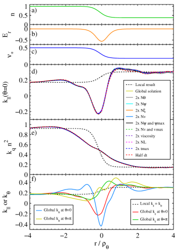
Figure 8: (Color online) a) Equilibrium density profile for the global calculation, normalized to its value at the left boundary. b) Normalized radial electric field $-cI(v_{\mathrm{i}}B_{0})^{-1}d\Phi_{0}/d\psi$. c) Profile of $\nu_{*}$. d) Parallel flow coefficient $k_{||}$, evaluated at the outboard midplane ($\theta=0$). Black dashed curve indicates the result of the local neoclassical code. The other curves (nearly indistinguishable) demonstrate the convergence of the global code to the various numerical resolution parameters. e) Radial heat flux, with the same legend as d). f) Normalized poloidal flow $k_{\theta}$ and $k_{||}$ evaluated at the outboard and inboard ($\theta=\pi$) midplanes.

For the parameters used here, $k_{||}$ and $k_{\theta}$ change sign in the simulation within the pedestal. These coefficients may have either sign in conventional theory, as shown in figure 2, depending on collisionality and magnetic geometry. In both the local and global cases, the integrand $v_{||}g$ that determines $k_{||}\propto\int d^{3}v\,v_{||}g$ is positive in part of phase space and negative elsewhere, and the balance between these regions determines the overall sign.

Structure with a radial scale comparable to $\rho_{\theta}$ is observed in the flow coefficients. Ions “communicate” over distances comparable to the orbit width $\sim\sqrt{\epsilon}\rho_{\theta}$, and so the effects of the driving electric field well are felt outside of the well itself, with influence decaying on the orbit width scale. The behavior of the flow coefficients on either side of the well need not be monotonic, as the mean flow adjacent to the well arises from a complicated interplay of particles entering from regions of differing collisionality, some particles directly affected by the electric field and some not.

The flow coefficients are also observed to be non-monotonic functions of $r$. This behavior is not unreasonable given the radial localization of the electric field well : even the local distribution function is a non-monotonic function of $r$, since it is a complicated function of the radially varying collisionality, so in the global case the flow coefficients need not be monotonic in $r$.

Figure 9 shows the poloidal variation of the flow coefficients near the pedestal top and bottom. As discussed in the appendix, the drift terms in the kinetic equation break the symmetry which the distribution function possesses in the local case, and so the flow coefficients need not be even or odd in $\theta$.

The various components of the mass conservation equation (26) were each independently computed from $g$: $\nabla\cdot\int d^{3}v\,v_{||}g\mbox{\boldmath$b$}$, $\nabla\cdot\int d^{3}v\,\mbox{\boldmath$v$}_{E0}g$, $\nabla\cdot\int d^{3}v\,\mbox{\boldmath$v$}_{\mathrm{m}}g$, and $\int d^{3}v\,S$. The first three of these integrals summed to nearly zero everywhere in space, with the sink integral negligible in magnitude compared to the others. Thus, the sink has little effect on the mass conservation relation that effectively determines the flows. The $\mbox{\boldmath$v$}_{\mathrm{m}}$ integral was intermediate in magnitude, leaving a dominant balance between the $\nabla\cdot\int d^{3}v\,v_{||}g\mbox{\boldmath$b$}$ and $\nabla\cdot\int d^{3}v\,\mbox{\boldmath$v$}_{E0}g$ terms. The density $\int d^{3}v\,g$ has a $\propto\cos(\theta)$ behavior in the pedestal, resulting in $\nabla\cdot\int d^{3}v\,\mbox{\boldmath$v$}_{E0}g\propto(\partial/\partial\theta)\int d^{3}v\,g\propto-\sin(\theta)$. To balance this term in the mass conservation law, $k_{||}$ must develop a $-\cos(\theta)$ structure, which can be seen in figure (9). Outside of the pedestal, the $\mbox{\boldmath$v$}_{E0}$ term becomes negligible due to the reduced $|d\Phi_{0}/d\psi|$, so this drive for poloidal variation in $k_{||}$ is absent.

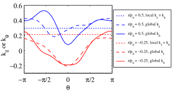
Figure 9: (Color online) Poloidal variation of the parallel flow coefficient $k_{||}$ and normalized poloidal flow $k_{\theta}$ at two radial locations straddling the pedestal.

Figure 10 shows how the results are altered when different choices are made for the sink. For the sink (54), we show results for $\gamma=0.1\omega_{\mathrm{t}}$ (the value used for all other plots) and for $\gamma=\omega_{\mathrm{t}}$. We also show results for the alternative sink (55). For comparison, results are also shown for a run in which no sink was included. For this run the code did not converge in time, due to the constant loss of heat described in section VIII, so it was stopped at $t=30\omega_{\mathrm{t}}$ (a time before the heat loss becomes excessive, but after the runs with sinks have nearly converged.) The various options yield results that show the same qualitative modification of the coefficients: a well develops in $k_{||}$ and $k_{\theta}$ at the outboard midplane, and the heat flux profile is flattened relative to the local prediction.

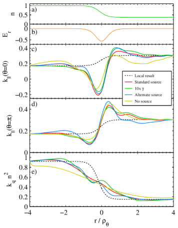
Figure 10: (Color online) Using the same equilibrium density profile (a) and $E_{r}$ profile (b) as in Figure (8), the parallel flow coefficients (c-d) and heat flux (e) show some minor dependence on the choice of sink. However, qualitative features such as the well in $k_{||}$ at the outboard midplane are robust.

As a further test of the code, we repeated the numerical calculation, treating $f_{1}$ as the unknown quantity instead of $g$ , in which case the inhomogeneous term in the equation is $-\mbox{\boldmath$v$}_{D}\cdot\nabla f_{\mathrm{Mi}}$ instead of $C_{\mathrm{i}}(F)$. Despite the very different phase-space structure of these two source terms, the numerical results from the two approaches agreed, as they should.

X Discussion

In this work we have demonstrated a method to extend neoclassical calculations to incorporate finite-orbit-width effects in a transport barrier for the case of $B_{\theta}\ll B$ (which is a good approximation in standard tokamaks) and a relatively weak ion temperature gradient. The method is implemented in a new continuum $\delta f$ code. Operator splitting is used to improve numerical efficiency, and we have demonstrated that excellent convergence is feasible for experimentally relevant parameters. By construction, the method exactly reproduces conventional (local) results in the appropriate limit of weak radial gradients. The Rosenbluth potentials are solved for along with the distribution function at each step, allowing use of the full linearized Fokker-Planck-Landau collision operator.

A principal finding of this work is that the parallel and poloidal flows may differ significantly from the conventional predictions. While the coefficients of the poloidal flow and $dT_{\mathrm{i}}/d\psi$-driven parallel flow are equal in conventional theory, in the pedestal these two coefficients ($k_{||}$ and $k_{\theta}$) differ. And, while the poloidal variation of the poloidal flow is $\propto B_{\theta}$ in the core, the same is not necessarily true in the pedestal. The poloidal variation of the flow is effectively determined by mass conservation, and in the pedestal, two new terms become important which are normally neglected: $\mbox{\boldmath$E$}\times\mbox{\boldmath$B$}$ convection of the poloidally varying density, and radial variation of the particle flux (which can be related to diamagnetic flow from the correction to the pressure). These effects cause the parallel flow coefficient $k_{||}$ to take a well-shaped radial profile, with different magnitude and (for some parameters) opposite sign, relative to the conventional local neoclassical result. In addition, the flow coefficients exhibit a strong poloidal variation not previously found. While this poloidal variation resembles $\cos(\theta)$, it contains other harmonics and is asymmetric about the midplane due to the magnetic drift.

These issues may be important for comparisons of experimental pedestal flows to theory Marr K D, Lipschultz B, Catto P J, McDermott R M, Reinke M L and Simakov A N (2010); Kagan G, Marr K D, Catto P J, Landreman M, Lipschultz B and McDemott R (2011). In general, the flow coefficients may differ in both magnitude and sign relative to local theory, as shown in figure 8. The fluid flow exhibits strong shear, with radial variation on the $\rho_{\theta}$ scale.

Associated with the modification to the flow, the parallel current is also modified. Due to the additional terms which must be included in the mass conservation equation, the usual division of the parallel current into Pfirsch-Schlüter and Ohmic-bootstrap components is modified, as shown in Eq. (44). In addition, the $dT_{\mathrm{i}}/d\psi$ contribution to the bootstrap current is altered, as shown in (45). In the $\delta f$ formulation, the ion temperature scale length cannot be as small as the density scale length in the pedestal, so these modifications to the parallel current are modest. However, similar changes to the current would presumably occur in a full-$f$ calculation when $r_{T}\sim\rho_{\theta}$, giving order-unity changes to the Pfirsch-Schlüter and bootstrap currents in that case. This issue needs to be examined in future studies.

In the development of this work, the local code was also used to test several analytic expressions for conventional neoclassical theory. The flow and heat flux coefficients $k_{||}=k_{\theta}=1.17,k_{q}=0.66$ derived using the momentum-conserving pitch-angle scattering model for collisions are a poor approximation unless $\epsilon$ is $\ll 0.1$. Expressions (16)-(17) are a much better approximation at realistic aspect ratio. The Chang-Hinton heat flux captures the trends at finite $\epsilon$ and $\nu_{*}$ well and gives results correct to within 20%, at least for the circular concentric flux surface model. The semi-analytic local formulae of Sauter et alSauter O, Angioni C, and Lin-Liu Y R (1999) for the flow and bootstrap current coefficients were found to be in excellent agreement with our local code when $\nu_{*}<0.3$, but some disagreement was found for $0.3<\nu_{*}<100$. For pedestal profiles typical of DIII-D, the Sauter bootstrap current formula closely agreed with our code at low collisionality, $\nu_{*e}<1$, but the Sauter formula can give a bootstrap current more than twice ours when $\nu_{*e}\geq 10$. The Sauter formulae are intended to reproduce results from a code based on the same physical model as our conventional local code.

There are many ways in which the global calculations can be extended. First, it would be useful to include impurities, for it is typically the impurity flow that is measured rather than that of the main ions, and the the flows of different ion species may be significantly different Ernst D R, Bell M G, Bell R E, Bush C E, Chang Z, Fredrickson E, Grisham L R, Hill K W, Jassby D L, Mansfield D K, McCune D C, Park H K, Ramsey A T, Scott D S, Strachan J D, Synakowski E J, Taylor G, Thompson M and Weiland R M (1998). Also, the presence of impurities can introduce a direct density gradient dependenceErnst D R, Bell M G, Bell R E, Bush C E, Chang Z, Fredrickson E, Grisham L R, Hill K W, Jassby D L, Mansfield D K, McCune D C, Park H K, Ramsey A T, Scott D S, Strachan J D, Synakowski E J, Taylor G, Thompson M and Weiland R M (1998) to $g$. Second, the method should be extended to allow strong temperature gradients ($r_{T}\sim\rho_{\theta}$). Doing so will require the full bilinear collision operator and a full-$f$ treatment. However, as the weak-$T_{\mathrm{i}}^{\prime}$ case is less complicated to analyze, due to the linearity of the kinetic equation, thorough understanding of this limit using the present approach is important for benchmarking future more sophisticated full-$f$ codes. Finally, studies of the velocity-space structure responsible for fluxes in turbulence codes may yield more accurate forms of the sink term needed in our approach.

Appendix A Null space and symmetry of the distribution

The local drift-kinetic equations (1) and (3) have two null solutions $f_{\mathrm{Mi}}$ and $v^{2}f_{\mathrm{Mi}}$, meaning that the discretized matrix for the local code should be nearly singular. In practice the matrix is still sufficiently well conditioned that the linear system may be solved without a problem, yielding a distribution function that contains a small amount of the two null solutions. For many applications this may not be a concern, because these null solutions do not contribute to the heat flux and flow.

For an up-down symmetric tokamak (i.e. if $B$ and $\nabla_{||}\theta$ are both unchanged under $\theta\to-\theta$), then a symmetry exists in the local kinetic equations: if $f_{1}(\theta,\xi,v)$ is a solution, then so is $-f_{1}(-\theta,-\xi,v)$ (and similarly for $g$). This property can be exploited to simultaneously eliminate the null space from the matrix and to reduce its sizeWong S K and Chan V S (2011). This is done by forcing $f_{1}$ to have the above symmetry by representing it as a sum of two types of modes: those that are even in $\theta$ and odd in $\xi$, and those that are odd in $\theta$ and even in $\xi$. The two null solutions do not possess this symmetry, so they are automatically excluded. Furthermore, the matrix size is reduced without loss of resolution. For example, the $\xi$ grid can be reduced to only cover the interval $[0,1]$ instead of $[-1,1]$ if all $\sin(M\theta)$ and $\cos(M\theta)$ modes are retained. The odd-$\theta$ (i.e. $\sin(M\theta)$) modes are forced to be even in $\xi$ by application of the boundary condition $\partial f_{1}/\partial\xi=0$ at $\xi=0$, and the even-$\theta$ (i.e. $\cos(M\theta)$) modes are forced to be odd in $\xi$ by application of the boundary condition $f_{1}=0$ at $\xi=0$.

Even if the parity of the solution is not enforced automatically by the discretization in this manner, the null solutions can still be excluded by enforcing parity as follows. Given a numerical solution $f_{1}(\theta,\xi,v)$ that contains some of the null solutions, the combination $\left[f_{1}(\theta,\xi,v)-f_{1}(-\theta,-\xi,v)\right]/2$ can be formed; the result will also satisfy the kinetic equation but have the desired parity.

In the global case, the symmetry of the kinetic equation is broken by the drift terms. However, the local operator has no null space in the initial-value-problem formulation due to the extra contribution on the matrix diagonal from the time derivative.

Appendix B Conservation laws for the global drift-kinetic equation

Here we sketch the derivation of general conservation equations, from which (26), (52), and (53) can be obtained. For most of this appendix we do not assume axisymmetry, we retain radial variation of magnetic quantities, and we do not require $\mbox{\boldmath$B$}\cdot\nabla\Phi=0$. We do require the electric field to be electrostatic and we assume $\partial\Phi/\partial t$ and $\partial\mbox{\boldmath$B$}/\partial t$ can be neglected. The derivation applies both to the full-$f$ and $\delta f$ contexts, since the necessary integrals of both the bilinear and linearized ion-ion collision operators vanish.

We begin with the ion drift-kinetic equation

$$\partial f_{\mathrm{i}}/\partial t+v_{||}\nabla_{||}f_{\mathrm{i}}+\mbox{\boldmath$v$}_{\mathrm{d}}\cdot\nabla f_{\mathrm{i}}=C\{f_{\mathrm{i}}\}+S$$ (56)

where $\mbox{\boldmath$v$}_{\mathrm{d}}=(v_{||}/\Omega)\nabla\times(v_{||}\mbox{\boldmath$b$})$ and $C$ is either the bilinear or linearized Fokker-Planck-Landau operator. Gradients are all performed at fixed $\mu$ and total energy $W=m_{\mathrm{i}}v^{2}/2+Ze\Phi$ (including the total potential $\Phi$, not just $\Phi_{0}$), so $\mbox{\boldmath$v$}_{\mathrm{d}}$ includes both the magnetic drift $\mbox{\boldmath$v$}_{\mathrm{m}}$ and $\mbox{\boldmath$E$}\times\mbox{\boldmath$B$}$ drift $\mbox{\boldmath$v$}_{E}$. This form of $\mbox{\boldmath$v$}_{\mathrm{d}}$ is convenient because it makes the kinetic equation conservative without cumbersome higher-order terms. This $\mbox{\boldmath$v$}_{\mathrm{d}}$ includes an incorrect $O(\beta)\ll 1$ parallel magnetic drift, but this component of the magnetic drift is typically unimportant compared to parallel streaming motion, and in fact $\mbox{\boldmath$v$}_{\mathrm{m}}\cdot\nabla\theta$ is precisely zero in the model magnetic geometry we use in the code. It is convenient to first rewrite

$$v_{||}\nabla_{||}f_{\mathrm{i}}+\mbox{\boldmath$v$}_{\mathrm{d}}\cdot\nabla f_{\mathrm{i}}=\frac{v_{||}}{B}\nabla\cdot\left(f_{\mathrm{i}}\mbox{\boldmath$B$}+\frac{m_{\mathrm{i}}c}{Ze}\frac{v_{||}}{B}\mbox{\boldmath$B$}\times\nabla f_{\mathrm{i}}\right).$$ (57)

Then $\int d^{3}v$ is applied to (56), annihilating $C$. Notice

$$\int d^{3}v=\frac{2\pi}{m_{\mathrm{i}}^{2}}\sum_{\sigma}\sigma\int_{Ze\Phi}^{\infty}dW\int_{0}^{(W-Ze\Phi)/B}d\mu\frac{B}{v_{||}}$$ (58)

where $\sigma=\mathrm{sgn}(v_{||})$. The divergence in (57) may be pulled in front of the integrals in (58), as the contributions from differentiating the integration limits all vanish either due to the $\sigma$ sum or because $v_{||}=0$ at the lower limit of $W$. Application of several vector identities to the $\mbox{\boldmath$B$}\times\nabla f_{\mathrm{i}}$ term then yields a mass conservation equation:

$$\frac{\partial}{\partial t}\left(\int d^{3}v\,f_{\mathrm{i}}\right)+\nabla\cdot\left(\int d^{3}v[v_{||}\mbox{\boldmath$b$}+\mbox{\boldmath$v$}_{\mathrm{d}}]f_{\mathrm{i}}\right)=\int d^{3}v\,S.$$ (59)

Flux surface averaging and neglect of $\Phi_{1}$ then gives (52).

An energy conservation equation may be obtained by observing that the above derivation of the mass conservation equation is essentially unchanged if $\int d^{3}v\,W$ is applied to (56) in place of $\int d^{3}v$. Subtracting $Ze\Phi\times$(59) from the result, one obtains

$$\frac{\partial}{\partial t}\left(\int d^{3}v\frac{m_{\mathrm{i}}v^{2}}{2}f_{\mathrm{i}}\right)+\nabla\cdot\left(\int d^{3}v[v_{||}\mbox{\boldmath$b$}+\mbox{\boldmath$v$}_{\mathrm{d}}]\frac{m_{\mathrm{i}}v^{2}}{2}f_{\mathrm{i}}\right)+\left(\int d^{3}v[v_{||}\mbox{\boldmath$b$}+\mbox{\boldmath$v$}_{\mathrm{d}}]f_{\mathrm{i}}\right)\cdot Ze\nabla\Phi=\int d^{3}v\frac{m_{\mathrm{i}}v^{2}}{2}S.$$ (60)

In the special case of axisymmetry and $\nabla_{||}\Phi=0$, flux surface averaging and integration in $\psi$ then gives (53).

To obtain the momentum conservation equation, it is convenient to specialize to axisymmetry at the start, taking the $\int d^{3}v(Iv_{||}/B)$ moment of (56), and using $\mbox{\boldmath$v$}_{\mathrm{d}}\cdot\nabla f_{\mathrm{i}}=(v_{||}/B)\nabla\cdot[f_{\mathrm{i}}(m_{\mathrm{i}}c/Ze)\nabla\times(v_{||}\mbox{\boldmath$b$})]$ instead of (57). The divergence may be brought in front of the $W$ and $\mu$ integrals as before. Noting $\mbox{\boldmath$v$}_{\mathrm{d}}\cdot\nabla(Iv_{||}/B)=0$ and $v_{||}\nabla_{||}(Iv_{||}/\Omega)=\mbox{\boldmath$v$}_{\mathrm{d}}\cdot\nabla\psi$, the result may be written

$$\frac{\partial}{\partial t}\left(\int d^{3}v\frac{Iv_{||}}{B}f_{\mathrm{i}}\right)+\nabla\cdot\left(\int d^{3}v\frac{Iv_{||}}{B}[v_{||}\mbox{\boldmath$b$}+\mbox{\boldmath$v$}_{\mathrm{d}}]f_{\mathrm{i}}\right)-\frac{Ze}{m_{\mathrm{i}}c}\int d^{3}v\,f_{\mathrm{i}}\mbox{\boldmath$v$}_{\mathrm{d}}\cdot\nabla\psi=\int d^{3}v\frac{Iv_{||}}{B}S.$$ (61)

This result holds in axisymmetry even if $\nabla_{||}\Phi$ and/or $\nabla_{||}I$ are nonzero.

Appendix C Convenient gauge

Here we prove that the gauge may always be chosen so

$$E_{||}=\frac{B}{\left<B^{2}\right>}\left<E_{||}B\right>-\nabla_{||}\Phi.$$ (62)

Axisymmetry is not required, and the loop voltage need not be uniform. The utility of (62) is that the inductive part of $E_{||}$ has simple spatial variation $\propto B$.

Suppose we begin in a different gauge, denoted by tildes, in which

$$\mbox{\boldmath$\tilde{E}$}=-c^{-1}\partial\mbox{\boldmath$\tilde{A}$}/\partial t-\nabla_{||}\tilde{\Phi}.$$ (63)

We may transform to a new gauge using $\Phi=\tilde{\Phi}-\partial\chi/\partial t$ and $\mbox{\boldmath$A$}=\mbox{\boldmath$\tilde{A}$}-\nabla\chi$ for a generator $\chi$. We choose

$$\chi=\int_{0}^{t}dt^{\prime}\int_{0}^{\theta}d\theta^{\prime}\frac{1}{\mbox{\boldmath$B$}\cdot\nabla\theta}\left[\frac{B^{2}}{\left<B^{2}\right>}\left<E_{||}B\right>+\frac{1}{c}\mbox{\boldmath$B$}\cdot\frac{\partial\mbox{\boldmath$\tilde{A}$}}{\partial t}\right]$$ (64)

where the integrand is evaluated at $t^{\prime}$ and $\theta^{\prime}$ rather than $t$ and $\theta$. We must verify (64) is single-valued in $\theta$ so $\Phi$ is single-valued. To this end, notice $\left<\mbox{\boldmath$B$}\cdot(\;\;\;)\right>$ applied to (63) gives $\left<E_{||}B\right>=-c^{-1}\left<\mbox{\boldmath$B$}\cdot\partial\mbox{\boldmath$\tilde{A}$}/\partial t\right>$. Therefore $\chi(\theta=2\pi)=0=\chi(0)$, so $\chi$ is indeed periodic. Applying $\nabla_{||}$ to $\Phi=\tilde{\Phi}-\partial\chi/\partial t$ with $\mbox{\boldmath$B$}\cdot$(63) and (64) then gives (62) as desired.

References

- Hinton F L and Hazeltine R D (1976) Hinton F L and Hazeltine R D, Rev. Mod. Phys. 48, 239 (1976).
- Helander P and Sigmar D J (2002) Helander P and Sigmar D J, Collisional Transport in Magnetized Plasmas (Cambridge University Press, Cambridge, 2002).
- Snyder P B and Wilson H R (2003) Snyder P B and Wilson H R, Plasma Phys. Controlled Fusion 45, 1671 (2003).
- Kagan G and Catto P J (2010a) Kagan G and Catto P J, Phys. Rev. Lett. 105, 045002 (2010a).
- Kim J, Burrell K H, Gohil P, Groebner R J, Kim Y-B, St John H E, Seraydarian R P and Wade M R (1994) Kim J, Burrell K H, Gohil P, Groebner R J, Kim Y-B, St John H E, Seraydarian R P and Wade M R, Phys. Rev. Lett. 72, 2199 (1994).
- Houlberg W A, Shaing K C, Hirshman S P and Zarnstorff M C (1997) Houlberg W A, Shaing K C, Hirshman S P and Zarnstorff M C, Phys. Plasmas 4, 3230 (1997).
- Ernst D R, Bell M G, Bell R E, Bush C E, Chang Z, Fredrickson E, Grisham L R, Hill K W, Jassby D L, Mansfield D K, McCune D C, Park H K, Ramsey A T, Scott D S, Strachan J D, Synakowski E J, Taylor G, Thompson M and Weiland R M (1998) Ernst D R, Bell M G, Bell R E, Bush C E, Chang Z, Fredrickson E, Grisham L R, Hill K W, Jassby D L, Mansfield D K, McCune D C, Park H K, Ramsey A T, Scott D S, Strachan J D, Synakowski E J, Taylor G, Thompson M and Weiland R M, Phys. Plasmas 5, 665 (1998).
- Crombe K, Andrew Y, Brix M, Giroud C, Hacquin S, Hawkes N C, Murari A, Nave M F F, Ongena J, Parail V, Van Oost G, Voitsekhovitch I and Zastrow K-D (2005) Crombe K, Andrew Y, Brix M, Giroud C, Hacquin S, Hawkes N C, Murari A, Nave M F F, Ongena J, Parail V, Van Oost G, Voitsekhovitch I and Zastrow K-D, Phys. Rev. Lett. 95, 155003 (2005).
- Solomon W M, Burrell K H, Andre R, Baylor L R, Budny R, Gohil P, Groebner R J, Holcomb C T, Houlberg W A and Wade M R (2006) Solomon W M, Burrell K H, Andre R, Baylor L R, Budny R, Gohil P, Groebner R J, Holcomb C T, Houlberg W A and Wade M R, Phys. Plasmas 13, 056116 (2006).
- Bell R E, Andre R, Kaye S M, Kolesnikov R A, LeBlanc B P, Rewoldt G, Wang W X and Sabbagh S A (2010) Bell R E, Andre R, Kaye S M, Kolesnikov R A, LeBlanc B P, Rewoldt G, Wang W X and Sabbagh S A, Phys. Plasmas 17, 082507 (2010).
- Marr K D, Lipschultz B, Catto P J, McDermott R M, Reinke M L and Simakov A N (2010) Marr K D, Lipschultz B, Catto P J, McDermott R M, Reinke M L and Simakov A N, Plasma Phys. Controlled Fusion 52, 055010 (2010).
- Kagan G, Marr K D, Catto P J, Landreman M, Lipschultz B and McDemott R (2011) Kagan G, Marr K D, Catto P J, Landreman M, Lipschultz B and McDemott R, Plasma Phys. Controlled Fusion 53, 025008 (2011).
- Rutherford P H (1970) Rutherford P H, Phys. Fluids 13, 482 (1970).
- Rosenbluth M N, MacDonald W M and Judd D L (1957) Rosenbluth M N, MacDonald W M and Judd D L, Phys. Rev. 107, 1 (1957).
- Hirshman S P and Sigmar D J (1976) Hirshman S P and Sigmar D J, Phys. Fluids 19, 1532 (1976).
- Belli E A and Candy J (2008a) Belli E A and Candy J, AIP Conf. Prof. 1069, 15 (2008a).
- Belli E A and Candy J (2008b) Belli E A and Candy J, Plasma Phys. Controlled Fusion 50, 095010 (2008b).
- Belli E A and Candy J (2009) Belli E A and Candy J, Plasma Phys. Controlled Fusion 51, 075018 (2009).
- Abel I G, Barnes M, Cowley S C, Dorland W and Schekochihin A A (2008) Abel I G, Barnes M, Cowley S C, Dorland W and Schekochihin A A, Phys. Plasmas 15, 122509 (2008).
- Catto P J and Ernst D R (2009) Catto P J and Ernst D R , Plasma Phys. Controlled Fusion 51, 062001 (2009).
- Belli E A and Candy J (2012) Belli E A and Candy J, Plasma Phys. Controlled Fusion 54, 015015 (2012).
- Wong S K and Chan V S (2011) Wong S K and Chan V S, Plasma Phys. Controlled Fusion 53, 095005 (2011).
- Sauter O, Harvey R W and Hinton F L (1994) Sauter O, Harvey R W and Hinton F L, Contrib. Plasma Phys. 34, 169 (1994).
- Sauter O, Lin-Liu Y R, Hinton F L and Vaclavik J (1994) Sauter O, Lin-Liu Y R, Hinton F L and Vaclavik J, Proceedings of the Theory of Fusion Plasmas workshop, Varenna (Editrice Compositori E. Sindoni, Bologna) , 337 (1994).
- Sauter O, Angioni C, and Lin-Liu Y R (1999) Sauter O, Angioni C, and Lin-Liu Y R, Phys. Plasmas 6, 2834 (1999).
- Kernbichler W, Kasilov S V, Leitold G O, Nemov V V and Allmaier K (2006) Kernbichler W, Kasilov S V, Leitold G O, Nemov V V and Allmaier K, 33rd EPS Conference on Plasma Phys., Rome 30I, P–2.189 (2006).
- Kernbichler W, Kasilov S V, Leitold G O, Nemov V V and Allmaier K (2008) Kernbichler W, Kasilov S V, Leitold G O, Nemov V V and Allmaier K, Plasma Fusion Res. 3, S1061 (2008).
- Lyons B C, Jardin S C, and Ramos J J (2012) Lyons B C, Jardin S C, and Ramos J J, Phys. Plasmas 19, 082515 (2012).
- Lin Z, Tang W M and Lee W W (1995) Lin Z, Tang W M and Lee W W, Phys. Plasmas 2, 2975 (1995).
- Lin Z, Tang W M and Lee W W (1997) Lin Z, Tang W M and Lee W W, Phys. Rev. Lett. 78, 456 (1997).
- Wang W X, Hinton F L and Wong S K (2001) Wang W X, Hinton F L and Wong S K, Phys. Rev. Lett. 87, 055002 (2001).
- Chang C S, Ku S and Weitzner H (2004) Chang C S, Ku S and Weitzner H, Phys. Plasmas 11, 2649 (2004).
- Wang W X, Tang W M, Hinton F L, Zakharov L E, White R B and Manickam J (2004) Wang W X, Tang W M, Hinton F L, Zakharov L E, White R B and Manickam J, Comp. Phys. Comm. 164, 178 (2004).
- Chang C S and Ku S (2006) Chang C S and Ku S, Contrib. Plasma Phys. 46, 496 (2006).
- Wang W X, Rewoldt G, Tang W M, Hinton F L, Manickam J, Zakharov L E, White R B and Kaye S (2006) Wang W X, Rewoldt G, Tang W M, Hinton F L, Manickam J, Zakharov L E, White R B and Kaye S, Phys. Plasmas 13, 082501 (2006).
- Kolesnikov R A, Wang W X, Hinton F L, Rewoldt G and Tang W M (2010) Kolesnikov R A, Wang W X, Hinton F L, Rewoldt G and Tang W M, Phys. Plasmas 17, 022506 (2010).
- Vernay T, Brunner S, Villard L, McMillan B F, Jollier S, Tran T M, Bottino A and Graves J P (2010) Vernay T, Brunner S, Villard L, McMillan B F, Jollier S, Tran T M, Bottino A and Graves J P, Phys. Plasmas 17, 122301 (2010).
- Xu X Q, Xiong Z, Dorr M R, Hittinger J A, Bodi K, Candy J, Cohen B I, Cohen R H, Colella P, Kerbel G D, Krasheninnikov S, Nevins W M, Qin H, Rognlien T D, Snyder P B and Umansky M V (2007) Xu X Q, Xiong Z, Dorr M R, Hittinger J A, Bodi K, Candy J, Cohen B I, Cohen R H, Colella P, Kerbel G D, Krasheninnikov S, Nevins W M, Qin H, Rognlien T D, Snyder P B and Umansky M V, Nucl. Fusion 47, 809 (2007).
- Xu X Q (2008) Xu X Q, Phys. Rev. E 78, 016406 (2008).
- Cohen R H, Dorf M, Compton J C, Dorr M, Rognlien T D, Colella P, McCorquodale P, Angus J and Krasheninnikov S (2012) Cohen R H, Dorf M, Compton J C, Dorr M, Rognlien T D, Colella P, McCorquodale P, Angus J and Krasheninnikov S, Bull. Am. Phys. Soc 57, BAPS.2012.APR.S1.38 (2012).
- R. J. Groebner and T. H. Osborne (1998) R. J. Groebner and T. H. Osborne, Phys. Plasmas 5, 1800 (1998), fig. 2.
- C.F. Maggi, R.J. Groebner, N. Oyama, R. Sartori, L.D. Horton, A.C.C. Sips,W. Suttrop and the ASDEX Upgrade Team, A. Leonard, T.C. Luce, M.R.Wade and the DIII-D Team, et al (2007) C.F. Maggi, R.J. Groebner, N. Oyama, R. Sartori, L.D. Horton, A.C.C. Sips,W. Suttrop and the ASDEX Upgrade Team, A. Leonard, T.C. Luce, M.R.Wade and the DIII-D Team, et al, Nucl. Fusion 47, 535 (2007).
- Y Corre, E Joffrin, P Monier-Garbet, Y Andrew, G Arnoux, M Beurskens, S Brezinsek, M Brix, R Buttery, I Coffey, et al (2008) Y Corre, E Joffrin, P Monier-Garbet, Y Andrew, G Arnoux, M Beurskens, S Brezinsek, M Brix, R Buttery, I Coffey, et al, Plasma Phys. Controlled Fusion 50, 115012 (2008).
- R. J. Groebner, T. H. Osborne, A. W. Leonard, and M. E. Fenstermacher1 (2009) R. J. Groebner, T. H. Osborne, A. W. Leonard, and M. E. Fenstermacher1, Nucl. Fusion 49, 045013 (2009).
- T. W. Morgan, H. Meyer, D. Temple, and G. J. Tallents (2010) T. W. Morgan, H. Meyer, D. Temple, and G. J. Tallents, in 37th EPS Conf. Plasma Phys. (Dublin, 2010) p. P5.122.
- A. Diallo, R. Maingi, S. Kubota, A. Sontag, T. Osborne, M. Podesta, R. E. Bell, B. P. LeBlanc, J. Menard, and S. Sabbagh (2011) A. Diallo, R. Maingi, S. Kubota, A. Sontag, T. Osborne, M. Podesta, R. E. Bell, B. P. LeBlanc, J. Menard, and S. Sabbagh, Nucl. Fusion 51, 103031 (2011).
- H. Meyer, M. F. M. De Bock, N. J. Conway, S. J. Freethy, K. Gibson, J. Hiratsuka, A. Kirk, C. A. Michael, T. Morgan, R. Scannell, et al (2011) H. Meyer, M. F. M. De Bock, N. J. Conway, S. J. Freethy, K. Gibson, J. Hiratsuka, A. Kirk, C. A. Michael, T. Morgan, R. Scannell, et al, Nucl. Fusion 51, 113011 (2011).
- A.C. Sontag, J.M. Canik, R. Maingi, J. Manickam, P.B. Snyder, R.E. Bell, S.P. Gerhardt, S. Kubota, B.P. LeBlanc, D. Mueller, T.H. Osborne and K.L. Tritz (2011) A.C. Sontag, J.M. Canik, R. Maingi, J. Manickam, P.B. Snyder, R.E. Bell, S.P. Gerhardt, S. Kubota, B.P. LeBlanc, D. Mueller, T.H. Osborne and K.L. Tritz, Nucl. Fusion 51, 103022 (2011).
- P. Sauter, T. Putterich, F. Ryter, E. Viezzer, E. Wolfrum, G.D. Conway, R. Fischer, B. Kurzan, R.M. McDermott, S.K. Rathgeber and the ASDEX Upgrade Team (2012) P. Sauter, T. Putterich, F. Ryter, E. Viezzer, E. Wolfrum, G.D. Conway, R. Fischer, B. Kurzan, R.M. McDermott, S.K. Rathgeber and the ASDEX Upgrade Team, Nucl. Fusion 52, 012001 (2012).
- R. Maingi, D.P. Boyle, J.M. Canik, S.M. Kaye, C.H. Skinner, J.P. Allain, M.G. Bell, R.E. Bell, S.P. Gerhardt, T.K. Gray, et al (2012) R. Maingi, D.P. Boyle, J.M. Canik, S.M. Kaye, C.H. Skinner, J.P. Allain, M.G. Bell, R.E. Bell, S.P. Gerhardt, T.K. Gray, et al, Nucl. Fusion 52, 083001 (2012).
- T. Pütterich, E. Viezzer, R. Dux, R. M. McDermott, and the ASDEX Upgrade team (2012) T. Pütterich, E. Viezzer, R. Dux, R. M. McDermott, and the ASDEX Upgrade team, Nucl. Fusion 52, 083013 (2012).
- R. M. McDermott, B. Lipschultz, J. W. Hughes, P. J. Catto, A. E. Hubbard, I. H. Hutchinson, R. S. Granetz, M. Greenwald, B. LaBombard, K. Marr, et al (2009) R. M. McDermott, B. Lipschultz, J. W. Hughes, P. J. Catto, A. E. Hubbard, I. H. Hutchinson, R. S. Granetz, M. Greenwald, B. LaBombard, K. Marr, et al, Phys. Plasmas 16, 056103 (2009).
- Kagan G and Catto P J (2008) Kagan G and Catto P J, Plasma Phys. Controlled Fusion 50, 085010 (2008).
- Li B and Ernst D R (2011) Li B and Ernst D R , Phys. Rev. Lett. 106, 195002 (2011).
- Catto P J, Bernstein I B and Tessarotto M (1987) Catto P J, Bernstein I B and Tessarotto M, Phys. Fluids 30, 2784 (1987).
- Chang C S and Hinton F L (1982) Chang C S and Hinton F L, Phys. Fluids 25, 1493 (1982).
- Taguchi M (1988) Taguchi M, Plasma Phys. Controlled Fusion 30, 1897 (1988).
- Hinton F L and Rosenbluth M N (1973) Hinton F L and Rosenbluth M N, Phys. Fluids 16, 836 (1973).
- Kagan G and Catto P J (2010b) Kagan G and Catto P J, Plasma Phys. Controlled Fusion 52, 055004 (2010b).
- Hazeltine R D (1973) Hazeltine R D, Plasma Phys. 15, 77 (1973).
- Lapillonne X, McMillan B F, Gorler T, Brunner S, Dannert T, Jenko F, Merz F and Villard L (2010) Lapillonne X, McMillan B F, Gorler T, Brunner S, Dannert T, Jenko F, Merz F and Villard L, Phys. Plasmas 17, 112321 (2010).