Two parameters scaling approach to Anderson localization of weekly interacting BEC

Abstract

We numerically study the Anderson localization of weekly interacting Bose-Einstein condensate in a one-dimensional disordered potential. We show that the interacting energy can not fully convert to the kinetic energy and two parameters are needed to describe such system completely, i.e., the density profile can be described with the sum of two exponential functions. This is a new attempt for precise description of systems with interplay of disorder and interaction.

I Introduction

Disorder is ubiquitous in nature that strongly affects the properties of many physical systems even it is only a weak perturbation. Fifty years ago, the localization of individual particles or waves in a disordered crystal was predicted by Anderson P.W.Anderson , and thus it is called Anderson localization (AL). It can be understood as an effect of multiple refection of a plane wave subject to random scattering or random potential barriers N.F.Mott . Later, AL has been unambiguously observed in many systems under the approximation of a single particle in a stationary disordered potential. For example, electromagnetic waves in photonic lattices with disorder T.Schwartz ; Y.Lahini and momentum distribution of quantum kicked rotor G.Casati1979 ; S.Fishman ; G.Casati1989 ; F.L.Moore ; J.Chabe . In single-particle approximation, the interaction among individual particles is not taken into consideration. However, real materials go far-beyond this approximation Lee ; B.Kramer , and thus observing AL is difficult. This can be understand as follows. Go beyond single-particle approximation, one needs to consider the interaction among particles. When this interaction induced nonlinear effect presences, the reflected waves will interfere with each other. Therefore, fully understanding the interplay of disorder and interaction is an extremely difficult task both experimentally and theoretically B.Kramer .

Ultracold quantum gas possesses unprecedented possibility of controlling almost all relevant physical parameters L.Sanchez-Palencia2007 ; L.Sanchez-Palencia2008 ; A.Aspect ; L.Sanchez-Palencia2010 ; G.Modugno ; Zhu2011 ; bs , and thus recognized as an ideal system for quantum simulation. A particularly interesting aspect of the system is implementing random speckle potential using laser beams R.Grimm ; J.M.Huntley ; P.Horak ; D.Cl ment ; Zhu2009 , which makes this system suitable for observing AL bs . Recently, two experimental groups have reported the observation of localization of a noninteracting as well as weak interacting Bose-Einstein condensate (BEC) in two different kinds of disordered potentials G.Roati ; J.Billy . The final state profile is theoretically described by a single parameter called localization length (LL) P.Lugan ; G.Kopidakis ; A.S.Pikovsky ; S.Flach ; Ch.Skokos . However, if disorder is switched on, different from Piraud’s work M. Piraud , interacting energy of BEC does not fully convert to kinetic energy when it stop to expand in a disorder potential. Therefore, the approach that interacting energy converts into kinetic energy completely L.Sanchez-Palencia2007 does not applicable for the center of the localized profile where interaction between particles can not be ignored. Similar scenario is expected in disorder induced AL, where one-parameter scaling theory is valid only for locally weak disorder sc . For strong disorder, the wavefunction is localized on just few sites and after that a very small exponential tail follows scp . This fact naturally leads us to consider AL with two parameters in interacting system. To exclude the effect induced from disorder, we consider the regime of week disorder, whcih one-parameter description is valid for disorder induced AL.

In this paper, we consider a concrete example of one-dimensional (1D) BEC with repulsive interaction in a random potential. We prove that two parameters description of AL in such system is more reasonable than that of single LL parameter. This is a new method to describe the localized profile, which provides a new method for studying AL with the interplay of disorder and interaction. The rest of this paper is arranged as following. In section II, we describes 1D BEC system with repulsive interaction, and shows that there is two different LL for the wing and center parts. In section III, as the wing LL is well known, we present detail study of the center LL focusing on its scaling law. In section IV, we give an approximate analytic expression linking the density profile of atom to the two LL and discuss the deviation of the expression. Finally, a brief summary is given in section V.

II Two parameters description of AL

Considering 1D BEC with repulsive interaction initially loaded in a harmonic trapping potential $V_{ho}(z)=\frac{1}{2}M\omega^{2}z^{2}$, where $M$ is the atomic mass and $\omega$ is the trapping frequency. The effective 1D structure can be achieved by applying an extremely tight harmonic vertical confinement to froze the atomic motion in the other two dimensions. The atomic interaction is effectively characterized by the $s$-wave scattering with effective 1D interacting strength labeled as $g$, which is experimentally tunable using the Feshbach resonance technique Chin . Here, one considers BEC in weakly interacting regime, i.e. $\overline{n}\gg Mg/\hbar^{2}$, where $\overline{n}$ is the average atomic density. Under the mean-field approximation, the dynamics of the considered system is governed by the following Gross-Pitaevskii (GP) equation

$$i\hbar\frac{\partial}{\partial t}\psi(z,t)=\left[\frac{\hat{p}_{z}^{2}}{2M}+V_{ext}(z)+g|\psi(z,t)|^{2}\right]\psi(z,t),$$ (1)

where $\hat{p}_{z}$ is the momentum operator, $V_{ext}(z)$ is the whole external potential, and the normalized wave function $\psi(z,t)$ is corresponding to a constant total number of atoms $N=\int|\psi(z,t)|^{2}dz$.

Now looking into the time-evolution of the BEC in a disordered external potential governed by Eq. (1). To this end, the procedures in the experiment J.Billy is followed: Firstly, prepare the 1D BEC at equilibrium of the harmonic potential without disorder, i.e., $V_{ext}(z)=V_{ho}(z)$. In the Thomas-Fermi (TF) regime ($\mu\gg\hbar\omega$), the initial wave function takes the form of an inverted parabola L.Sanchez-Palencia2008

$$\psi(z,0)=\sqrt{\left({\mu\over g}\right)\left(1-{z^{2}\over L_{TF}^{2}}\right)}\Theta\left(1-{|z|^{2}\over L_{TF}^{2}}\right),$$ (2)

where $\mu$ is the chemical potential, $L_{TF}=\sqrt{2\mu/\omega^{2}}$ is the TF half-length and $\Theta$ denotes the Heaviside step function. Secondly, at time $t=0$, one switches off the harmonic potential and applies a disorder potential along the expanding axis (i.e. $z$ axis) of the BEC. It also assumes that the disorder potential $V_{d}(z)$ is generated by laser speckle method as in the experiment J.Billy . It is a random potential with a truncated negative exponential single-point distribution J.W. Goodman :

$$P[V(z)]=\frac{\exp[-(V(z)+V_{R})/V_{R}]}{V_{R}}\Theta\left(\frac{V(z)}{V_{R}}+1\right),$$ (3)

The average of disorder potential is set to be $\langle V_{d}(z)\rangle=0$ and its correlation function $C(z)=\langle V_{d}(z^{\prime})V_{d}(z^{\prime}+z)\rangle=V_{R}^{2}c(z/\sigma_{R})$, which $c(u)=\sin^{2}(u)/u^{2}$, $V_{R}=\sqrt{\langle V_{d}^{2}\rangle}$ is the standard deviation and $\sigma_{R}$ is the correlation length. Thus the external potential after $t=0$ is given by $V_{ext}(z)=V_{d}(z)$. In the case of $\sigma_{R}/\xi_{int}<1$ that $\xi_{int}=\sqrt{4M\mu}$ is the initial healing length of BECs, the density profile of the BEC will take a form of an exponential-decay function when experiencing enough time J.Billy .

To investigate the AL of the system, the time evolution of the atomic density profile $n(z,t)=|\psi(z,t)|^{2}$ is worked out

$$\psi(z,t)=\hat{T}\exp\left(-\frac{i}{\hbar}\int_{0}^{t}H_{GP}dt\right)\psi(z,0),$$ (4)

where the GP Hamiltonian is $H_{GP}=\frac{\hat{p}^{2}_{z}}{2M}+V_{d}(z)+g|\psi(z,t)|^{2}$ and $\hat{T}$ is the time ordering operator. $\psi(z,t)$ is numerically calculated by using the standard operator-split method. According to Ref. Larson , Eq. (4) can be rewritten as

$$\psi(z,t+\delta t) = \left\{\exp\left({-\frac{i\hat{p}^{2}_{z}}{4M\hbar}\delta t}\right)\right.$$

$$\times\exp\left\{{-\frac{i}{\hbar}\left[V_{d}(z)+g|\psi(z,t)|^{2}\right]\delta t}\right\}$$

$$\left.\times\exp\left({-\frac{i\hat{p}^{2}_{z}}{4M\hbar}\delta t}\right)+\mathcal{O}({\delta t}^{3})\right\}\psi(z,t),$$

where the high-order term $\mathcal{O}({\delta t}^{3})$ comes from the non-commuting relation of the terms in $H_{GP}$. In the sufficiently short time step $\delta t$, this term can be safely neglected. Combining with the Fourier transform between the position and momentum spaces, we can finally get the numerical solution of $\psi(z,t)$ following the computation procedure step by step with time step $\delta t$.

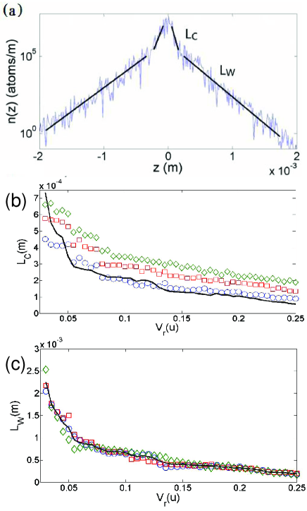
Figure 1: (Color online) (a) The stationarity of the localized profile with disorder potential strength $V_{R}=0.15\mu$, nonlinear intensity $Ng/h=0.035$ Hz, total number of atoms $N=1.7\times 10^{4}$ and $\sigma_{R}/\xi_{int}\approx 0.65$. We can define two different LLs. Central LL (b) and Wing LL (c) versus amplitude of the disordered potential in different nonlinear intensity: $Ng/h$=0.035Hz (blue $\times$), 0.104Hz (red $\nabla$), 0.204Hz (green $\circ$). All LLs are obtained in an evolution time $t=2$ s. The black line indicate the case of no interaction.

When experiencing long enough time, the BEC will stop expanding. As $\sigma_{R}\ll L_{TF}$, the expanding of BEC is experienced with vast random oscillation of potential. Due to disorder averaging, as shown in Fig. 1(a), the final density profile of BEC takes the form of exponential-like function in a large scale. It is find that the wing of density profile can be exponentially fit by a wing LL denoted as $L_{W}$ in Fig. 1(a), which has been considered as the single parameter to characterize LL of the system in experiment J.Billy and takes the analytic form of L.Sanchez-Palencia2007

$$L_{W}=\frac{2\hbar^{4}}{\pi M^{2}V_{R}^{2}\sigma_{R}\xi_{int}^{2}(1-\sigma_{R}/\xi_{int})}.$$ (6)

However, the profile of the center part of BEC is not fit the form of $L_{W}$ as shown in Fig. 1(a), which is also the case in Fig. (1) of the experiment in Ref. J.Billy . In the experiment, the profile of center part of BEC is also stationary and do not fit the form of $L_{W}$. Further analysis indicates that the result of this special center profile is that the interacting energy does not convert kinetic energy completely, i.e., this profile does not correspond to the standard AL.

In order to analyze it, one introduces a center LL denoted as $L_{C}$, which is defined by the length in $z$ axis which reduces the maximum value of the finial wave function by a factor of $1/e$. When the interaction strength is weak ($Ng/h=0.035$ Hz), two LLs can be approximately unified and the system may be described by the single parameter theory L.Sanchez-Palencia2007 , which is verified by the very good agreement of the black line and the green circle plot as shown in Fig. 1(b) and 1(c). However, for stronger interaction ($Ng/h=0.104$ Hz), both in experiment J.Billy and our simulation in Fig. 1(b) indicate that the central part of the density profile can not be characterized by $L_{W}$ though it is also localized. To describe the AL of the central part of the BEC, center LL is needed.

Furthermore, the trend of two LLs is studied by changing the amplitude of the disordered potentials in different nonlinear interaction intensity $Ng$. The results, as shown in Fig.1(b) and 1(c), show that the two LLs both nearly exponentially decrease with the increasing of the amplitude of the disordered potentials, but interestingly, they exhibit different behavior: $L_{W}$ is insensitive to the nonlinear intensity as expected from Eq. (6), but $L_{C}$ is strongly affected by it. This can be understand by the facts: i) for larger amplitude of the disordered potential, AL is more significant, and thus both LLs are smaller; and ii) the impact of $g|\psi(z)|^{2}$ on the wing part $L_{W}$ is slight, but significant for the center part $L_{C}$ since the density of this part is much larger than that of the wing part [cf. Fig. 1(a)]. It needs emphasizing that the extend of center part is much larger than $\sigma_{R}$, so it also undergo multiple refection random potential, which is AL characteristics.

III A scaling law of $L_{C}$

In contrast to the single-parameter scaling theory for the disorder system in liner regime, here two LLs as localization parameters are needed to describe this nonlinear disorder system completely. The difference in this nonlinear system is that BEC finally reach nearly equilibrium in the disorder potential, and then the wing part can be well described by the LL for the noninteracting cases. However, the central part still contains certain residual interaction energy, and thus the LL of this part would be different.

Obviously, $L_{C}$ is relate to interaction. And numerically calculate finds that $L_{C}$ as a function of the nonlinear interaction intensity $Ng$. As shown in Fig. 2(a), one finds that $L_{C}$ approximately linearly depends on $\sqrt{Ng}$, i.e.

$$L_{C}\propto\sqrt{Ng}+constant,$$ (7)

for a disorder potential with fixed $V_{R}$. For small $V_{R}$ cases, there are some variances in the fitting (cf. Fig. 2(a)). Considering the particle number $N$ with normalization equation

$$N = \int_{-\infty}^{\infty}|\psi(z,0)|^{2}dz=\int^{L_{TF}}_{-L_{TF}}\frac{u}{g}\left(1-\frac{z^{2}}{L_{TF}^{2}}\right)dz$$ (8)

$$= \frac{4\mu L_{TF}}{3g},$$

one can obtain the expression of the TF half-length as $L_{TF}=3Ng/4\mu$. It implies a relation $L_{C}\propto\sqrt{L_{TF}}$. Combining with the dimensional analysis, it is natural to guess that there may be a relationship between $L_{C}$ and $\sqrt{L_{TF}}\times\sqrt{L_{W}}$. Through a simple fitting, It is find that $L_{C}$ has an interesting scaling law of

$$L_{C}\simeq\sqrt{L_{W}L_{TF}},$$ (9)

as shown in Fig. 2(b).

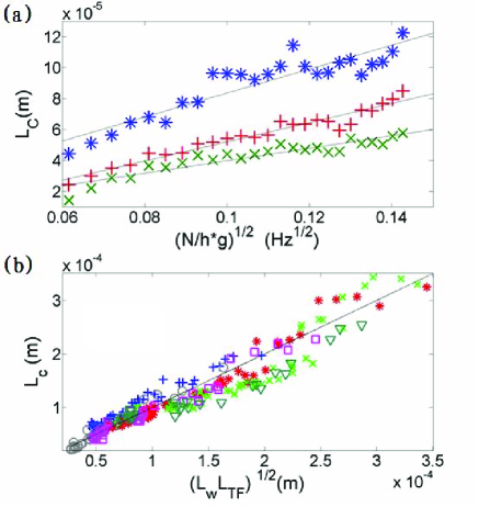
Figure 2: (Color online) (a) The $L_{C}$ versus $\sqrt{g}$ in different $V_{R}$: $V_{R}$=0.1u (blue $\ast$), 0.2u(red $+$), 0.3u(green $\times$) with black lines are theoretical predicted results by Eq. (6). (b) The $L_{C}$ versus the $\sqrt{L_{W}L_{TF}}$. They are obtained different nonlinear intensity: Ng/h=0.035Hz (blue $\times$), 0.104Hz (red $\ast$), 0.204Hz (green +), and different evolution time: 2.1s (gray $\circ$), 4.5s (purple $\oblong$), 7.0s (dark green $\nabla$). The solid line is the function $y=x$.

It is showed some analysis about the physics picture of Eq.(9). $L_{W}$ can be taken as a main measurement of the strength of localization of the system, thus $L_{C}$ as an additional measurement should be positively related to $L_{W}$. Since the central part of BEC can not fully expand and has less kinetic energy, it is less sensitive to the strength of localization than the wing part does. Therefore, its power index is less than $1$ and exhibits $L_{C}\propto\sqrt{L_{W}}$. Additionally, $L_{TF}$ is a measurement of the size and the profile of the initial state, and then $L_{C}$ could also be positively related to $L_{TF}$. Because of the disorder potential and the smaller kinetic energy, the power index is also less than $1$ and exhibits $L_{C}\propto\sqrt{L_{TF}}$.

IV An approximate analytic expression of density profile

The previous analysis shows that its finial density profile takes the form of

$$n(z,\tau)\propto\begin{cases}\exp(-2|z|/L_{C})&\text{$|z|\leq z_{0}$}\\ \exp(-2|z|/L_{W})&\text{$|z|>z_{0}$}\end{cases},$$ (10)

where $z_{0}$ is the theoretical cross-point. Here $z_{0}$ is difficult to determine, so a simple form is assumed

$$n_{a}(z,\tau)=\frac{N-\Lambda}{L_{W}}\exp(-2|z|/L_{W})+\frac{\Lambda}{L_{C}}\exp(-2|z|/L_{C})$$ (11)

to describe the full density profile, where $\Lambda$ is an undetermined coefficient. In the following we will see that $\Lambda$ can be approximately determined.

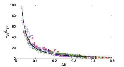
Figure 3: (Color online) The scale parameter $L_{W}/L_{TF}$ versus the residual interaction energy $\triangle E$ with $\sigma_{R}/\xi_{int}=0.65$. $L_{W}/L_{TF}$ is obtained from different nonlinear intensity: 0.104Hz (red $\ast$), 0.204Hz (green +), and different evolution time: 2.1s (gray $\circ$), 4.5s (purple $\oblong$), 7.0s (dark green $\nabla$). The solid line is the best fit with the function in the Eq.(10).

As the interaction energy does not transform kinetic energy completely, considering normalized residual interaction energy $\Delta E$ to characterize this, which is defined as

$$\Delta E = \frac{g\int|\psi(z,\tau)|^{2}dz}{g\int|\psi(z,0)|^{2}dz}$$ (12)

$$= \frac{5}{6N^{2}}\left[\Lambda^{2}\beta+(N-\Lambda)^{2}\beta^{2}+\frac{4(N-\Lambda)}{\beta^{2}+\beta}\right],$$

where $\tau$ is the typical time scale when the BEC is nearly stable, and $\beta=\sqrt{L_{TF}/L_{W}}$. Considering Eq.(9), Eq.(12) can become a simple form. For the single LL cases, i.e. $\Lambda=0$ in Eq. (12), It can find that $\Delta E=5L_{TF}/6L_{W}$. Based on the numerical simulation, It also finds that there is a well fitting formula to characterize the relationship between $\Delta E$ and $L_{w}/L_{TF}$ for our two LLs description, as shown in Fig. 3. The fitting formula is given by

$$\frac{L_{W}}{L_{TF}}\simeq\triangle E^{-\frac{4}{3}}.$$ (13)

This relation can be understood by the fact that $L_{W}$ and $L_{TF}$ are the characteristic lengths of finial and initial states, and thus their ratio may has certain connection with the residual interaction energy, which is the ratio of the interaction energy of final and initial states. If the BEC expands fully, the residual interaction energy tends to zero and $L_{W}$ will be much larger than $L_{TF}$, corresponding to $\Delta E\rightarrow 0$ for $L_{W}/L_{TF}\rightarrow\infty$ in Eq. (13) (cf. Fig. 3). On the other hand, if the expansion is relatively very small, comparable to the initial length scale of the BEC, then $L_{W}$ will be nearly equivalent to $L_{TF}$, corresponding to the residual interaction energy tends to unit.

Substituting Eq. (13) into Eq. (12), one can work out $\Lambda$, which is approximately given by

$$\Lambda\simeq\left[0.75\left(\frac{L_{TF}}{L_{W}}\right)^{0.1}+0.04\right]N$$ (14)

Up to this, the full density profile of the localized BEC can be characterized by Eq. (11) and Eq.(14).

Due to Eq.(13) and Eq.(14) are approximate, it is need to investigate the deviation in the determining $L_{C}$ by using Eq. (10) and Eq. (11). To this end, $z_{1}$ and $z_{2}$ ($z_{1}$, $z_{2}$$<z_{0}$) are definded as the solutions of $n(z_{1},\tau)=n_{a}(z_{2},\tau)$ in the central part (i.e. $z_{1,2}<L_{C}$):

$$\left(\frac{N-\Lambda}{L_{W}}+\frac{\Lambda}{L_{C}}\right)e^{-2\frac{z_{1}}{L_{C}}}=\frac{N-\Lambda}{L_{W}}e^{-2\frac{z_{2}}{L_{W}}}+\frac{\Lambda}{L_{C}}e^{-2\frac{z_{2}}{L_{C}}}.$$ (15)

and deviation $\delta z=(z_{2}-z_{1})/z_{1}$. $\delta z>0$ indicate the distribution of our approximation is wider than the precise distribution in the z-direction , and vice versa. According to Eqs. (13, 14, 15), the deviation $\delta z$ as a function of $\Delta E$ and $z_{1}$ is showed in Fig. 4. And it can find that when $\Delta E$ is in the small and large sides the deviation is smaller than that in the intermediate regime. However, the deviation using our approximation is always less than $18\%$ in the whole regime. Relatively speaking, for non-interacting system, both the deviation of the experimental and theoretical values are larger than $50\%$ J.Billy . While for the interacting system, the deviation predicted in Ref. L.Sanchez-Palencia2007 is larger than $60\%$ with the same parameters of Fig. (1) when $V_{R}$ is in the small and large sides. Therefore, It can conclude that Eq. (11) of $n_{a}$ is a better approximation to describe the density profile of the localized BEC in a wide parameter range.

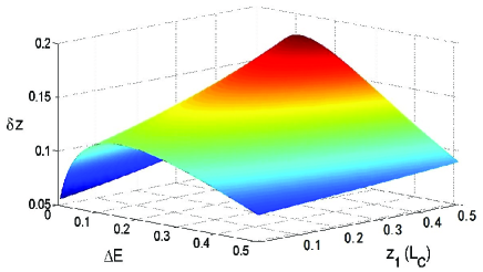
Figure 4: (Color online) The parameter $\delta z$ versus the residual interaction energy $\triangle E$ and $z_{1}/L_{C}$.

V Conclusion

In summary, we have demonstrated that it is better and more completely to use double LLs to describe the AL of 1D weekly interacting BECs in a disordered potential. We furthermore find a scaling law related to the relationship between the newly defined LL and the nonlinear atomic interactions. An approximate analytic form of the full density profile of the localized BEC is also proposed by using the two LLs.

References

- (1) P. W. Anderson, Phys. Rev 109, 1492 (1958).
- (2) N. F. Mott and J. Non-Cryst, Solids 1, 1 (1968).
- (3) T. Schwartz, G. Bartal, S. Fishman, and M. Segev, Nature 446, 52 (2010).
- (4) Y. Lahini, R. Pugatch, F. Pozzi, M. Sorel, R. Morandotti, N. Davidson, and Y. Silberberg, Phys. Rev. Lett. 103, 013901 (2009).
- (5) G. Casati, B. V. Chirikov, F. M. Izraelev, and J. Ford, Stochastic Behavior in Classical and Quantum Hamiltonian Systems (Lecture Notes in Physics vol 93, Berlin: Springer, 1979).
- (6) S. Fishman, D. R. Grempel, and R. E. Prange, Phys. Rev. Lett. 49, 509 (1982).
- (7) G. Casati, I. Guarneri, and D. L. Shepelyansky, Phys. Rev. Lett.62, 345 (1989).
- (8) F. L. Moore, J. C. Robinson, C. F. Bharucha, B. Sundaram, and M. G. Raizen, Phys. Rev. Lett. 75, 4598 (1995).
- (9) J. Chabe, G. Lemarie, B. Gremaud, D. Delande, P. Szriftgiser, and J. C. Garreau, Phys. Rev. Lett. 101, 255702 (2008).
- (10) P. A. Lee and T. V. Ramakrishnan, Rev. Mod. Phys. 57, 287 (1985).
- (11) B. Kramer and A. MacKinnon, Rep. Prog. Phys. 56, 1469 (1993).
- (12) L. Sanchez-Palencia, D. Clement, P. Lugan, P. Bouyer, G. V. Shlyapnikov, and A. Aspect, Phys. Rev. Lett. 98, 210401 (2007).
- (13) S.-L. Zhu, L. B. Shao, Z. D. Wang, and L.-M. Duan, Phys. Rev. Lett. 106, 100404 (2011); S.-L. Zhu, B. Wang, and L.-M. Duan, ibid 98, 260402 (2007).
- (14) L. Sanchez-Palencia, D.Clement, P. Bouyer and A.Aspect, New J. Phys. 10 045019 (2008).
- (15) A. Aspect and M. Inguscio, Phys. Today 62, 30 (2009).
- (16) L. Sanchez-Palencia and M. Lewenstein, Nature Phys 6, 87 (2010).
- (17) G. Modugno, Rep. Prog. Phys. 73, 102401 (2010).
- (18) B. Shapiro, J. Phys. A 45, 143001 (2012).
- (19) J. M. Huntley, Appl. Opt. 28, 4316 (1989).
- (20) P. Horak, J.-Y Courtois, and G. Grynberg, Phys. Rev. A 58, 3953 (1998).
- (21) R. Grimm, M. Weidemüller, and Yu. B. Ovchinnikov, Adv. At. Mol. Opt. Phys. 42, 95 (2000).
- (22) D. Clément, A.F. Varón, J. A. Retter, L. Sanchez-Palencia, A. Aspect, and P. Bouyer, New J. Phys. 8, 165 (2006).
- (23) S.-L. Zhu, D.-W. Zhang, and Z. D. Wang, Phys. Rev. Lett. 102, 210403 (2009).
- (24) G. Roati, C. D’Errico, L. Fallani, M. Fattori, C. Fort, M. Zaccanti, G. Modugno, M. Modugno, and M. Inguscio, Nature 453, 895 (2008).
- (25) J. Billy, V. Josse, Z. Zuo, A. Bernard, B. Hambrecht, P. Lugan, D. Clement, L. Sanchez-Palencia, P. Bouyer, and A. Aspect, Nature 453, 891 (2008).
- (26) J.W. Goodman, in Statistical Properties of Laser Speckle Patterns, edited by J.-C. Dainty, Laser Speckle and Related Phenomena (Springer-Verlag, Berlin, 1975).
- (27) P. Lugan, D. Clement, P. Bouyer, A. Aspect, M. Lewenstein, and L. Sanchez-Palencia, Phys. Rev. Lett. 98, 170403 (2007).
- (28) G. Kopidakis, S. Komineas, S. Flach, and S. Aubry, Phys. Rev. Lett. 100, 084103 (2008).
- (29) A. S. Pikovsky and D. L. Shepelyansky, Phys. Rev. Lett. 100, 094101 (2008).
- (30) S. Flach, D. O. Krimer, and C. Skokos, Phys. Rev. Lett. 102, 024101 (2009); S.-L. Zhu and Z. D. Wang, ibid, 85, 1076 (2000).
- (31) C. Skokos and S. Flach, Phys. Rev. E. 82, 016208 (2010).
- (32) M. Piraud, P. Lugan, P. Bouyer A. Aspect and L. Sanchez-Palencia, Phys. Rev. A. 83, 031603 (2011).
- (33) A. Cohen, Y. Roth, and B. Shapiro, Phys. Rev. B 38, 12125 (1988).
- (34) B. Shapiro, private communication.
- (35) C. Chin, R. Grimm, P. Julienne, and E. Tiesinga, Rev. Mod. Phys. 82, 1225 (2010).
- (36) J. Larson and E. Sjoqvist, Phys. Rev. A 79, 043627 (2009), and the references there in.