Spectral Optical Monitoring of the Narrow Line Seyfert 1
galaxy Ark 564

Abstract

We present the results of a long-term (1999–2010) spectral optical monitoring campaign of the active galactic nucleus (AGN) Ark 564, which shows a strong Fe II line emission in the optical. This AGN is a narrow line Seyfert 1 (NLS1) galaxies, a group of AGNs with specific spectral characteristics. We analyze the light curves of the permitted H$\alpha$, H$\beta$, optical Fe II line fluxes, and the continuum flux in order to search for a time lag between them. Additionally, in order to estimate the contribution of iron lines from different multiplets, we fit the H$\beta$ and Fe II lines with a sum of Gaussian components. We found that during the monitoring period the spectral variation (F_max/F_min) of Ark 564 was between 1.5 for H$\alpha$ to 1.8 for the Fe II lines. The correlation between the Fe II and H$\beta$ flux variations is of higher significance than that of H$\alpha$ and H$\beta$ (whose correlation is almost absent). The permitted-line profiles are Lorentzian-like, and did not change shape during the monitoring period. We investigated, in detail, the optical Fe II emission and found different degrees of correlation between the Fe II emission arising from different spectral multiplets and the continuum flux. The relatively weak and different degrees of correlations between permitted lines and continuum fluxes indicate a rather complex source of ionization of the broad line emission region.

1 Introduction

Narrow-line Seyfert 1 (NLS1) galaxies were first introduced as a class of active galactic nuclei (AGNs) by Osterbrock & Pogge (1985). Their optical spectra show relatively narrow (FWHM $\leq$ 2000 km s^-1) permitted lines, which are narrower than in a typical Seyfert 1 galaxy. In particular, Osterbrock & Pogge (1985) did show that, the permitted lines are only slightly broader than the forbidden ones, and that a strong Fe II emission is present in the optical region of the spectrum. In addition, the [O III] $\lambda$5007/H$\beta$ ratio, emitted in the narrow line region (NLR), varies from 1 to 5 (Rodríguez-Ardila et al., 2000), instead of the universally adopted observed value for Seyfert 1s of around 10 (Rodríguez-Ardila et al., 2000), indicative of the presence of high-density gas. Osterbrock & Pogge (1985) pointed out that the H$\beta$ equivalent widths in NLS1s are smaller than typical values for normal Seyfert 1s, suggesting that they are not just normal Seyfert 1s seen at a particular viewing angle. Renewed interest in NLS1s arises from the discovery of their distinctive X-ray properties: they show a steep X-ray excess with a photon index of 3 below 100 keV, a steep hard X-ray continuum, and a rapid large-amplitude X-ray variability on timescales of minutes to hours (see Leighly, 1999a, b, 2000; Panessa et al., 2011, and references therein). Moreover, optical studies have established that NLS1s lie at one end of the Boroson & Green (1992) eigenvector 1 (EV1) and that they show a relatively strong Fe II emission and a weak [O III] emission (Boller et al., 1996). They also represent the ”extreme Population A” objects (FWHM H$\beta<$ 4000 km/s) as defined by the four dimensional eigenvector 1 (4DE1) in Sulentic et al. (2007); Marziani et al. (2010). 4DE1 involves four parameters and NLS1 are ”extreme” in all of them: they have the narrowest broad H$\beta$, strongest Fe II emission, strongest X-ray excess and largest C IV blueshifts.

Arakelian 564 (Ark 564, IRAS 22403+2927, MGC +05-53-012) is a bright $V=14.6$ mag. (de Vaucouleurs et al., 1991), nearby narrow-line Seyfert 1 galaxy ($z=0.02467$), with an X-ray luminosity $L_{2-10\rm keV}=2.4\times 10^{43},\rm{erg\ s^{-1}}$ (Turner et al., 2001). This AGN is one of the brightest NLS1s in the X-ray band (Boller et al., 1996; Collier et al., 2001; Smith et al., 2008), and it shows a soft excess below $\sim$1.5 keV and a peculiar emission-line-like feature at 0.712 keV in the source rest frame (Chiho et al., 2004). The variations of the X-ray amplitude in the short-timescale light curve is very similar to those in the long-timescale light curve (Pounds et al., 2001), that is in contrast to the stronger amplitude variability on longer timescales, which is a characteristic of broad-line Seyfert 1 (BLS1) galaxies. In the UV part of the spectrum, this galaxy shows intrinsic UV absorption lines (Crenshaw et al., 1999). In order to explore the variability characteristics of a NLS1 in different wavelength bands, a multiwavelength monitoring campaign of Ark 564 was conducted (Shemmer et al., 2001). The optical campaign covered the periods 1998 November – 1999 November and 2000 May – 2001 January, where the object was observed both photometrically (UBVRI filters) and spectrophotometrically (spectral coverage 4800–7300 Å) (Shemmer et al., 2001). The data set and analysis is described in details and compared with the simultaneous X-ray and UV campaigns (Shemmer et al., 2001). The results of this intensive variability multiwavelength campaign show that the optical continuum is not significantly correlated with the X-ray emission (Shemmer et al., 2001). The UV campaign, carried out with the HST on 2000 May 9 and 2000 July 8, is described in Collier et al. (2001). These authors found a small fractional variability amplitude of the continuum between 1365 Å  and 3000 Å  (around  6%), but reported that large-amplitude short-timescale flaring behavior is present, with trough-to-peak flux changes of about 18% in approximately 3 days (Collier et al., 2001). The wavelength-dependent continuum time delays in Ark 564 have been detected and these delays may indicate a stratified continuum reprocessing region (Collier et al., 2001).

Here we present the long-term monitoring of Ark 564 in the optical part of the spectrum. We analyzed the variability in the permitted emission lines and continuum in order to determin the size and structure of emitting regions of the permitted Balmer and Fe II lines. We placed particular interest in the strong Fe II lines of the H$\beta$ spectral region whose behavior is investigated in details and discussed in this paper.

The paper is organized as follow: in section 2 we describe the observations and data reduction procedures, in section 3 we give an analysis of the spectral data, in section 4 we explore the correlations between different lines and the continuum, as well as between different lines, in section 5 we investigate in more details the Fe II variation, in section 6 we discuss our results, and in section 7 we provide our conclusions.

2 Observations and data reduction

Spectral monitoring of Ark 564 was carried out with the 6 m and 1 m telescopes of the SAO RAS (Russia, 1999–2010), the INAOE’s 2.1 m telescope of the ”Guillermo Haro Observatory” (GHO) at Cananea, Sonora, México (1999–2007), and the 2.1 m telescope of the Observatorio Astronómico Nacional at San Pedro Martir (OAN-SPM), Baja California, México (2005–2007). Spectra were taken with long–slit spectrographs equipped with CCDs. The typical observed wavelength range was 4000–7500 Å, the spectral resolution was R=5–15 Å, and with S/N ratio $>$ 50 in the continuum near H$\alpha$ and H$\beta$. In total 100 blue and 55 red spectra were obtained during 120 nights. In the analysis, about 10% of spectra were discarded for several different reasons: e.g. a) large noise (S/N$<$15Å - 2001 Aug 29 (blue, red), 2001 Oct 08 (blue), 2001 Oct 09 (blue, red), taken with Zeiss(1m)+CCD(1k$\times$1k); b) large noise and badly corrected spectral sensitivity in the blue part - 2006 Jun 28 (blue, red), 2006 Aug 29(blue), 2006 Aug 30 (blue), 2009 Aug 14 (blue), 2009 Oct 11 (blue), taken with Zeiss(1m)+CCD(2k$\times$2k). We note here that the CCD(2k$\times$2k) sensitivity in the blue part is not good enough, since it is a red CCD; c) poor spectral resolution (R$>$20Å, - 2003 Nov 18, 2004 Oct 18, taken with 2.1m GHO). Thus our final data set consisted of 91 blue and 50 red spectra, which were used in further analysis.

From 1999 to 2003 spectral observations with 1 m Zeiss telescope of the SAO were carried out with two different CCDs (formats used were 1k$\times$1k or 530$\times$580) and the H$\alpha$ and H$\beta$ spectral regions were observed separately. From 2004 to 2010 a CCD (2k$\times$2k, EEV CCD42-40) was used, allowing us to observe the entire wavelength range (4000–8000) Å  with a spectral resolution of 8-10 Å. However, this CCD in the blue part of some spectra presents large sensitivity variations (i.e. bad S/N), which are badly corrected, thus the blue region of these spectra was not used in our analysis.

From 2004 to 2007, the spectral observations with two Mexican 2.1 m telescopes were carried out with two observational setups. In the case of GHO observations we used the following configuration: 1) with a grating of 150 l/mm (spectral resolution of R=15 Å, a resolution similar to the observations of 1999–2003); 2) with a grating of 300 l/mm (moderate spectral resolution of R=7.5Å). The similar spectral characteristics at the OAN-SPM were, respectively, obtained with the following configuration: 1) with a grating of 300 l/mm (spectral resolution of R=15 Å); 2) with a grating of 600 l/mm (moderate spectral resolution of R=7.5Å).

As a rule, observations were carried out with the moderate resolution in the blue or red bands during the first night of each run. In order to cover H$\alpha$ and H$\beta$ at the same time, we used the lower resolution mode and observed the entire spectral range 4000-7500 Å; and then the moderate resolution was adopted again for the following night. Since the shape of the continuum of active galaxies practically does not change during adjacent nights, it was easy to match, the blue and red bands obtained with the moderate resolution in different nights. To this aim we used the data obtained for the continuum from the low-dispersion spectra for the entire wavelength range. By this procedure, the photometric accuracy is thus considerably improved with respect to a match obtained by overlapping the extremes of the blue and red continuum (3-5% instead of 5-10%).

Spectrophotometric standard stars were observed every night.

Information on the source of spectroscopic observations is listed in Table 1. The log of the spectroscopic observations is given in Table 2. Taking into account all observations, the mean sampling rate is 33.20, and the median rate is 2.95 days. The big difference between the mean and median sampling rate is due to the big gaps in the variability campaign.

The spectrophotometric data reduction was carried out either with the software developed at the SAO RAS or with the IRAF package for the spectra obtained in México. The image reduction process included bias and flat-field corrections, cosmic ray removal, 2D wavelength linearization, sky spectrum subtraction, addition of the spectra for every night, and relative flux calibration based on observations of standard star.

2.1 Absolute calibration (scaling) of the spectra

The standard technique of flux calibration of the spectra (i.e. comparison with stars of known spectral energy distribution) is not precise enough for the study of AGN variability, since even under good photometric conditions, the accuracy of spectrophotometry is usually not better than 10%. Therefore we used standard stars only to provide a relative flux calibration. Instead, for the absolute calibration, the observed fluxes of the forbidden, narrow emission lines are adopted for the scaling procedure the AGN spectra, since these fluxes are expected to be constant (Peterson, 1993). From HST observations (Crenshaw et al., 2002) it was shown that the NLR in Ark 564 is about $0.2$” (95 pc), and this facts implies a constant [OIII]$\lambda$5007 flux intensity during several hundred years. Consequently, the flux of this forbidden line should not have changed during our monitoring period. The scaling of the blue spectra was performed using the method of Van Groningen & Wanders (1992) modified by Shapovalova et al. (2004). We will not repeat the scaling procedure here, we only note that the flux in the lines was determined after subtraction of a linear continuum determined by the beginning and the end of a given spectral interval. This method allowed us to obtain a homogeneous set of spectra with the same wavelength calibration and the same [OIII]$\lambda$5007 flux. The [OIII]$\lambda$5007 flux in absolute units was taken from Shemmer et al. (2001): F([OIII]$\lambda$5007)=(2.4$\pm$0.1)$\times 10^{-13}\rm erg\ s^{-1}cm^{-2}$. The spectra, obtained with 2.1 m telescopes in Mexico with a resolution of 12–15 Å, containing both H$\alpha$ and H$\beta$ regions were scaled using the [O III]$\lambda$5007 line. However, some spectra of Ark 564 were obtained separately in the blue (H$\beta$) and red (H$\alpha$) wavelength bands, with a resolution of 8–10 Å. Usually, the red edge of the blue spectra and the blue edge of the red spectra overlap in an interval of 300 Å. Therefore, first the red spectra (17) were scaled using the overlapping continuum region with the blue ones. The latter were scaled with the [OIII]$\lambda$5007 line. In these cases the scaling uncertainty was about 5%–10%. Then scaling of the red spectra was refined using the mean flux in [OI]$\lambda$6300 (mean F[OI]$\lambda$6300$\sim$(1.93$\pm$0.24)$\times 10^{-14}$), determined from low-dispersion spectra (R$\sim$12–15 Å). For 3 red spectra (JD:2452886.9; 2455058.5 and 245116.4) we have no blue spectrum in adjacent nights, and they was scaled using only the mean flux of the [OIII]$\lambda$6300Å line.

2.2 Unification of the spectral data

In order to investigate the long term spectral variability of an AGN, it is necessary to conform a consistent, uniformed data set. Since observations were carried out with 4 different instruments, we must correct the line and continuum fluxes for aperture effects (Peterson & Collins, 1983). To this effect, we determined a point-source correction factor $\varphi$ given by the following expression (see Peterson et al., 1995, for a detailed discussion):

$$F({\rm H}\beta)_{\rm true}=\varphi\cdot F({\rm H}\beta)_{\rm obs}$$

where $F({\rm H}\beta)_{\rm obs}$ is the observed H$\beta$ flux; $F({\rm H}\beta)_{\rm true}$ is the aperture corrected H$\beta$ flux. The contribution of the host galaxy to the continuum flux depends also on the aperture size. The continuum fluxes $F(5235$Å) (in the observed-frame) were corrected for different amounts of host-galaxy contamination, according to the following expression (see Peterson et al. (1995)):

$$F(5235\AA)_{\rm true}=\varphi\cdot F(5235\AA)_{\rm obs}-G(g),$$

where $F(5235$Å$)_{\rm obs}$ is the continuum flux at 5235 Å  in the observed-frame; $G(g)$ is an aperture-dependent correction factor to account for the host galaxy contribution. The GHO observing scheme (Table 1), which correspond to a projected aperture ($2.5^{\prime\prime}\times 6^{\prime\prime}$) of the 2.1 m telescope, were adopted as standard (i.e. $\varphi=1.0$, $G(g)$=0 by definition). The correction factors $\varphi$ and $G(g)$ are determined empirically by simulated aperture photometry of suitable images of the narrow line emission and the starlight of the host galaxy in the same way as it is given in Peterson et al. (1995). This procedure is accomplished empirically by comparing pairs of simultaneous observations from each of given telescope data sets to that of the standard data set (as it used in AGN Watch, e.g. Peterson et al., 1994, 1999, 2002). As noted in these papers, even after scaling of the spectra to a common value of the [OIII] 5007 flux, there are systematic differences between the light curves produced from the data obtained with different telescopes. Therefore, it is proposed to correct for small offsets between the light curves from different sources in a simple, but effective fashion (e.g. Peterson et al., 2002, and references therein), attributing these small relative offsets to aperture effects (Peterson et al., 1995). The procedure also corrects for other unidentified systematic differences between data sets (for example, miscentering of the AGN nucleus in spectrograph aperture, etc.). In our paper we took the GHO-data as standard, because this data set contains the largest number of observed spectra. The correction factors $\varphi$ and $G(g)$ are determined empirically by comparing pairs of nearly simultaneous observations from each of the given telescope data sets (L(U), SPM, Z1K, Z2K) to that of the GHO data set. In practice, intervals which we defined as ”nearly simultaneous” are typically of 1-2 days. Therefore, the variability on short time scales ($<2$ days) is suppressed. The point-source correction factors $\varphi$ and $G(g)$ values for different samples are listed in Table 3. Using these factors, we re-calibrated the observed fluxes of H$\alpha$, H$\beta$, Fe II 48,49 and continuum to a common scale corresponding to our standard aperture $2.5^{\prime\prime}\times 6^{\prime\prime}$ (Table 4).

2.3 Measurements of the spectra and errors

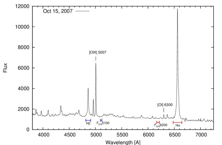
Figure 1: An example of the total optical spectrum of Ark 564. The windows for H$\beta$, H$\alpha$, blue and red continuum measurements are marked.

From the scaled spectra we determined the average flux in the blue continuum at the rest-frame wavelength $\sim 5100$ Å, by means of flux averages in the spectral interval 5094–5123 Å in the rest-frame (Table 5). We also calculated the average flux in the red continuum at the rest-frame wavelength $\sim 6200$ Å, by averaging the flux in the spectral interval 6178–6216 Å in the rest-frame (Table 5). These intervals wavelength were selected because they do not contain noticeable emission lines (Fe II or any other lines, see Fig. 1).

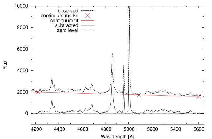
Figure 2: Underlying continuum subtraction in the H$\beta$ region needed for accurate Fe II measurements.

In order to determine the observed fluxes of the H$\alpha$, H$\beta$ and Fe II lines we need to subtract the underlying continuum, thus, a linear continuum was defined through 20 Å windows, located at rest-frame wavelengths 4762 Å  (4880 Å in the observed-frame) and 5123 Å  (5250 Å in the observed-frame) for the H$\beta$ line, and at rest-frame wavelengths 6334 Å (6490 Å in the observed-frame) and 6656 Å (6820 Å in the observed-frame) for the H$\alpha$ line (Fig. 1). In the case of Fe II emission, a precise subtraction of the underlying continuum for a larger wavelength range is required. Hence, a polynomial fit for the continuum was drawn through continuum windows (Fig. 2) located at the rest-frame wavelength intervals 4210–4230 Å, 5080–5100 Å, 5600–5630 Å, (see e.g. Kuraszkiewicz et al., 2002; Kovačević et al., 2010).

After the continuum subtraction, we measured the observed fluxes of the emission lines in the following rest-frame wavelength intervals: 4817–4909 Å  for H$\beta$, 6480–6646 Å  for H$\alpha$, and 5100–5470 Å  for the Fe II emission (hereafter Fe II red shelf). The measurements are given in Table 5. In this Fe II wavelength range, mainly the 48 and 49 Fe II multiplets are located (Fig. 2), yet there is also a contribution of the 42 multiplet around 5170 Å in the rest-frame (see Kovačević et al., 2010). This spectral interval was chosen because the Fe II lines there included are not blended with other either strong broad and narrow emission lines (e.g. He II 4686 Å). This allows to determine the Fe II line fluxes in a straightforward manner (Fig. 2). Further in the text, we discuss a more detailed analysis of the Fe II emission in a wider spectral interval 4100–5600 Å in the rest-frame (see Section 5).

Worth noting, is the fact that the H$\beta$ and H$\alpha$ fluxes here reported, include the corresponding narrow component fluxes: in the case of H$\beta$ – only the narrow H$\beta$ is included (the [OIII]$\lambda\lambda$4959,5007 lines are out from the H$\beta$ spectral interval); while for H$\alpha$ case – lines of [NII]$\lambda\lambda$6548, 6584 and narrow H$\alpha$ are included. As fluxes of narrow lines are assumed to be constant, they have no influence on the broad line component variability. The line and continuum fluxes were corrected for aperture-effect using the listed correction factors in Table 3 (see Subsection 2.2).

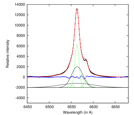
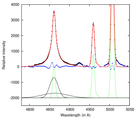
Figure 3: The best Gaussian fitting (solid line) of the mean H$\alpha$ (left) and H$\beta$ (right) line profiles (dotted line) with a sum of Gaussians. The broad components are fitted with two Gaussian (solid lines) and the narrow lines with one (dashed lines). The line residuals are also given below the observed spectra. In the region of the H$\beta$ the Fe II contribution is not subtracted.

In Table 4 the fluxes for the blue continuum (at 5100 Å), H$\alpha$, H$\beta$ and Fe II lines are listed. We have also estimated the flux contribution from the H$\beta$ and H$\alpha$ narrow components and [NII]$\lambda\lambda$6548, 6584, from multi Gaussian fit to the blends (H$\beta$+[OIII]$\lambda\lambda$4959,5007 and H$\alpha$+[NII]$\lambda\lambda$6548,6584) of the mean profiles. The best fits are plotted in Fig. 3. From the mean spectra, the estimated contribution of F(H$\beta$) narrow component to the total line flux is $\sim$20%. The narrow F(H$\alpha$) has a contribution of about 30% while the fluxes of the [NII]$\lambda\lambda$6548,6584 a 7% one. A similar result (an averaged contribution of $\sim$18%) was obtained for the F(H$\beta$) narrow component from the gaussian fit to every blue spectrum (see section 5).

Additionally, we measured line-segment fluxes. In doing this, we divided the H$\alpha$ and H$\beta$ line profiles into three parts: a blue wing, a core and a red wing. The adopted intervals in wavelength and velocity are listed in Table 5.

The mean uncertainties (errorbars) for the fluxes of continuum, H$\alpha$ and H$\beta$ lines, and their line segments (wings and core) are listed in Table 5. These quantities were estimated from the comparison of the results of spectra obtained within a time interval shorter than 3 days. The details of evaluation techniques of these uncertainties (errorbars) are given in Shapovalova et al. (2008). As can be notices, in Table 5 the mean error of the continuum flux, total H$\alpha$, H$\beta$ lines and their cores, is $\sim$4%. While due to their relatively weaker flux, the errors in the determination of the fluxes of the Fe II and line wings are larger, about $\sim$(7–9)%.

3 Results of the data analysis

3.1 Variability of the emission lines and of the optical continuum

We analyzed flux variations in the continuum and emission lines from a total of 91 spectra covering the H$\beta$ wavelength region, and 50 spectra covering the H$\alpha$ line vicinity. In Fig. 4 the blue continuum subtracted spectrum of Ark 564, obtained with the 6 m SAO telescope in November 23, 2001 (JD 2452237.1) is presented. There, we marked the positions of some relevant Fe II multiplets (27,28,37,38,42,48,49) and other important emission lines. As it can be easily noticed, the Fe II emission is rather strong, as it is usually the case in NLS1 galaxies.

From the flux data listed in Table 4, we obtained light curves for the blue and red continua, and for H$\alpha$, H$\beta$, and Fe II emission (Fig. 5), and their line-segments (blue wing, core, and red wing, Fig. 6). As one can see in Figs. 5 and 6, the fluxes declined slowly from the beginning to the end of the monitoring period. For H$\alpha$ and H$\beta$ a decline of $\sim$20% is present, while, for the Fe II emission, a decline of $\sim$30% and one of $\sim$40% for the continuum flux are seen (Fig. 5). In the upper panel of Fig. 5, the upper dashed line represents the flux at the beginning of the monitoring campaign, and the lower dashed line at the end of it. There is only one red point in 2010 at which point the red flux increased (two lower panels in Fig. 5). Similarly as in Collier et al. (2001), the light curves show several flare-like increments (see Fig. 5). The light curves of line wings and core (Fig. 6) show practically simultaneous variations. There might be up to five flare-like events detected in our data (see Table 6) when the flux increases $\sim$10-20% for a short period of time ($\sim$1-3 days, Table 6), out of which two flares were prominent: in December 2003 and August 2004. As it can be seen from Table 6, as a rule, flare-like events in the continuum (see dF(cnt) in %) are stronger than in emission lines.

Long-term flux-monitoring programs have shown that the flux variations of AGNs tend to be stochastic (i.e., there are few cases of periodicity or quasi-periodicity, see e.g. Shapovalova et al., 2010). However, the AGN light curves sometimes, as in the case of Ark 564, can show a flare-like characteristics whose spectral properties are consistent with a shot-noise process (Cruise & Dodds, 1985; Hufnagel & Bregman, 1992; Hughes et al., 1992). One way to reproduce shot noise is through a superposition of a series of identical impulses, occurring at intervals dictated by Poisson statistics. In a Poisson process, the overall rate of events is statistically constant, yet the starting times of individual events are independent of all previous ones. The time intervals between events follow an exponential distribution. It is possible to use such a process in Ark 564 variability investigation, by assuming a constant flare rate $\rho$, and let $Tj$ be the occurrence time of the $j$-th flare. Probability of no occurrence of flare in the interval $[Tj,Tj+\tau]$ is $exp(-\rho\tau)$.

The probability that a second flare will occur within a time $\tau$ after the first one is $p(\tau)=1-exp(-\rho\tau)$. Actually, we can say that $p[Tn+1-Tn<\tau|T0,T1,...Tn]=1-exp(-\rho\tau)$ means that at least one flare does occur between $Tn$ and $Tn+\tau$.

As it can be seen from Table 6, in the continuum and H$\beta$ we have 4 events in 4 separate years which gives a density of events in 10-year long monitoring period of 0.4 events per year. In such a way we could estimate probability of time between flare events (which could be recorded in the continuum flux and H$\beta$ line) as $p(\tau)=1-exp(-0.4\tau)$. As for H$\alpha$, we have 3 events in 3 separate years over 10 years period, which leads to $p(\tau)=1-exp(-0.3\tau)$. Finally, in the case of Fe II line we have 5 events in 4 separate years (2 events occurred at the end of October 2006), so we could take $\rho=3/10+2/10=1/2$, which leads to $p(\tau)=1-exp(-0.5\tau)$. The exponential density is monoton decreasing; hence there is a high probability of a short interval, and a small probability of a long interval between flares. This means that typically we will have flares occurring close to each other and spaced out by long, but rare intervals with no occurrence of flares.

In Table 7 we list several parameters characterizing the variability of the continuum, total line, and line-segments fluxes. There are several methods to estimate variability, here we will use the method given by O’Brien et al. (1998). There $F$ denotes the mean flux over the whole observing period and $\sigma(F)$ its standard deviation. $R$(max/min) is the ratio of the maximal to minimal fluxes in the monitoring period. $F$(var) is a inferred (uncertainty-corrected) estimate of the variation amplitude with respect to the mean flux, defined as:

$$F({\rm var})=[\sqrt{\sigma(F)^{2}-e^{2}}]/F({\rm mean})$$

$e^{2}$ being the mean square value of the individual measurement uncertainty for N observations, i.e. $e^{2}=\frac{1}{N}\sum_{i}^{N}e(i)^{2}$ (O’Brien et al., 1998).

From Table 7 one can see that the amplitude of variability $F$(var) is $\sim$10% for the continuum and Fe II emission and $\sim$7.5% for the total H$\beta$ flux. The H$\beta$ blue wing shows slightly larger variability (F(var)$\sim$15%) than the red one (F(var)$\sim$11%, see Table 7). However, the H$\alpha$ line wings and core show lower amplitude variability (F(var)$\sim$8%) than the H$\beta$ wings (F(var)$\sim$(11-15)%).

3.2 Mean and Root-Mean-Square Spectra

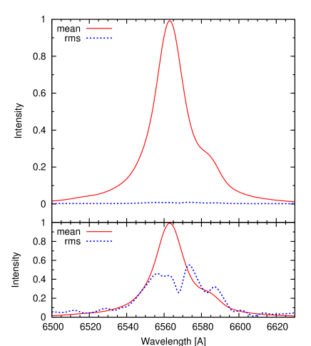
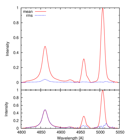
Figure 7: The mean and rms spectra of H$\alpha$ (left) and H$\beta$ (right) after calibrating the spectra to the same spectral resolution. Below plots show the normalized mean and rms spectra arbitrary scaled for comparison.

We calculated the mean H$\alpha$ and H$\beta$ line profiles and their root-mean-square (rms) profiles. To find the different portion of variability in different line parts, as much as it is possible, first we inspect the spectra and conclude that the spectra with spectral resolution $\leq$11 Å for H$\alpha$ and $\leq$10 Å for H$\beta$ are good enough for this purpose, thus having a sample of 23 red spectra and 61 blue spectra (Fig. 7). For this purposes the spectra were calibrated to have the same spectral resolution (11 Å for H$\alpha$ and 10 Å for H$\beta$).

Fig. 7 shows that the H$\alpha$ and H$\beta$ line profiles in Ark 564 are Lorentzian like (with broad wings), that is a characteristic of the NLS1 galaxies (see e.g. Sulentic et al., 2009, 2011). The rms profile of H$\beta$ resembles a Lorentzian like one, while in case of H$\alpha$ there is practically no change in the profile. The FWHM of the H$\beta$ line from the observed mean and rms profiles is 960 km/s, and from the observed mean profile of H$\alpha$ is 800 km/s. The full width at Zero Intensity (FW0I) of H$\beta$ is much more difficult to measure since the Fe II emission contributes to the red wing. Thus we only give estimates of FWOI of H$\beta$ mean profiles (or rms) to be $\sim$8000 and for H$\alpha$ is also $\sim$8000 km/s. As it can be seen in Fig. 7, the rms is relatively weak ($F_{\rm rms}({\rm H}\alpha)/F_{\rm H\alpha}\sim 0.01$ and $F_{\rm rms}({\rm H}\beta)/F_{\rm H\beta}\sim 0.07$), meaning that there are no significant changes in the line profiles of H$\alpha$ and H$\beta$ during the monitoring period. Note here that we did a recalibration of the H$\beta$ line taking that the [OIII] lines have the same profile during the monitoring period, therefore we have small rms in forbidden lines, but it is also interesting that the rms shape of H$\beta$ is practically the same as the total H$\beta$ (composed from the broad and narrow components, see Fig. 3). This may indicate that the whole (Lorentzian-like) line is emitted from a complex BLR and that the contribution of the narrow component, that is coming from the same region as the [OIII] lines, is negligible. On the other hand, the H$\alpha$ line rms shows that the variability is caused mainly by variations in the line wings.

4 The continuum vs. line flux correlations

To determine whether there are any changes in the structure of the broad-line region (BLR), we investigated both the relationships between the total line flux of H$\alpha$, H$\beta$ and Fe II and different line-segments (wings and core) of H$\alpha$ and H$\beta$.

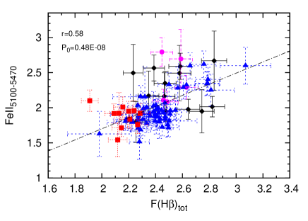
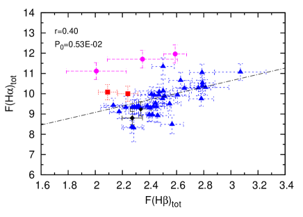
Figure 8: The Fe II red shelf (left) and H$\alpha$ (right) line fluxes as a function of the H$\beta$ line flux. The correlation coefficient and the corresponding P-value are given in the upper left corner. The notation is the same as in Fig. 5.

In Fig. 8 the correlations between the total line flux of H$\beta$, H$\alpha$ and Fe II are presented. It is interesting to note that the correlations between the flux variation of H$\beta$ and H$\alpha$ is significantly weaker (r$\sim$0.40, and it seems statistically insignificant with P=0.0053) than that with the Fe II (r$\sim$0.58, and P$<10^{-8}$). The lack of correlations between the H$\alpha$ and H$\beta$ fluxes may indicate a very complex BLR structure. On the other hand, the correlation between different line-segment fluxes (i.e. blue/red wing-core, blue wing-red wing) are better, especially for H$\alpha$ (Fig. 9).

In Fig. 10 we present the relationships between the continuum flux at 6200 Å (for H$\alpha$) and 5100 Å (for H$\beta$) and the total line and line-segment fluxes for H$\alpha$ and H$\beta$. As it can be seen in Fig. 10 the correlation between line and continuum fluxes are weak. Such weak linear correlations of the lines with continuum may indicate existence of different sources of ionization (AGN source - photo-ionization, shock-impact excitation and etc.). It is interesting to note that the Fe II emission seems to show a slightly better correlation with the continuum at 5100 Å (r$\sim$0.76, and P$<10^{-16}$) than Balmer lines (Fig. 11).

4.1 Balmer decrement

We have calculated the BD=F(H$\alpha$)/F(H$\beta$) flux ratio, i.e. the Balmer decrement (see Fig. 12), using $\sim$50 blue and red spectra taken in the same night (or one night before or after). We obtained a mean Balmer decrement value BD(mean)=4.396$\pm$0.369, and no significant changes in the monitoring period. In Fig. 12 the BD against the continuum flux is shown, and it can be seen there is no correlation between the BD and continuum (R$\sim$0.02). It is apparent that the BD was more or less constant during the 11-year monitoring period. The ratio of H$\alpha$ and H$\beta$ depends on the physics in the BLR, and in the low density regime, the H$\alpha$/H$\beta$ ratio is expected to be below 4 and it has a slight dependence on temperature (see discussion and Figs. 6 and 7 in Ilić et al., 2012). In the high density regime, the H$\alpha$/H$\beta$ ratio starts to depend on the temperatrue (see Ilić et al., 2012). The obtained mean BD for Ark 564 seems to be close to the high density regime, and changes in the BD from 3.5 to 5.5 might be caused by an inhomogeneous BLR, i.e. may indicate a stratified BLR in density, temperature and rate of ionization.

4.2 Lags between continuum and permitted lines

In order to determine potential time lags between the continuum and permitted line changes, we calculated the cross-correlation function (CCF) for the continuum light curve with the emission-line light curves. There are several ways to construct a CCF, and it is always advisable the use of two or more methods to confirm the obtained results. Therefore, we cross-correlated the 5100 Å continuum light curve with both the H$\beta$ and H$\alpha$ line (and Fe II emission) light curves using two methods: (i) the z-transformed discrete correlation function (ZDCF) method introduced by Alexander (1997), and (ii) the interpolation cross-correlation function method (ICCF) described by Bischoff & Kollatschny (1999).

The time lags calculated by ZDCF are given in Table 8, where it can be seen that inferred lags have large associated errors. It is interesting to note that the Fe II lines tend to have shorter lag values, while the longest one is that of the H$\alpha$ line. If one takes a direct conversion from the time lag to the BLR size, the expected BLR sizes are of an order of $10^{-3}$ parsecs (0.003 to 0.0055 pc) that indicate a compact BLR, but also a strong stratification in the emitting region of Ark 564, where the Fe II emitting region tends to be very compact and the largest one is the H$\alpha$ emitting line region. We also calculated the lags using the ICCF and found a delay between the continuum and H$\beta$ line of $\sim$6.7 days, and between the continuum and Fe II emission of about 0 days, that is in agreement with the ZDCF method (see Table 8). The errors are around 10 lightdays.

The uncertainties in the delays inferred from the CCFs are difficult to estimate, especially the evaluation of a realistic error of the CCF. In our case, the main problem in the time delay determination, likely comes from the small variation detected in lines and continuum fluxes (see Table 7) and also their weak correlations (see Figs. 10 and 11). Therefore, all obtained lag times should be taken with caution.

5 Variation of the Fe II lines

As mentioned above, the strong Fe II emission is one of the main characteristics for NLS1 galaxies. Optical Fe II ($\lambda\lambda$4400–5400) emission is one of the most interesting features in AGN spectra. The emission arises from numerous transitions of the complex Fe II ion (see Kovačević et al., 2010, for more details). The iron emission is seen in almost all type-1 AGN spectra and it is especially strong in the NLS1s. The origin of the optical Fe II lines, their excitation mechanisms, and the spatial location of the Fe II emission region in AGNs are still open questions (see e.g. Popović et al., 2009; Kovačević et al., 2010; Popović & Kovačević, 2011). There are also many correlations between the Fe II emission and other AGN properties which require a physical explanation. As discussed above, we found that Fe II lines show a slightly better correlation with the continuum at 5100 Å than Balmer lines (Fig. 11). On the other hand, it seems that the H$\beta$ line flux is better correlated with the Fe II emission, than with H$\alpha$. We should note here that this better correlation might be caused by the fact that the Fe II fluxes are much more susceptible to the contamination from the continuum emission than the H$\alpha$ and H$\beta$ lines.

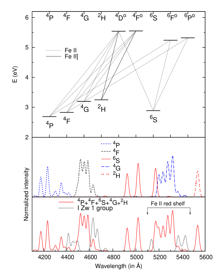
Figure 13: The simplified Grotrian diagram showing the strongest Fe II transitions in the $\lambda\lambda$ 4100-5600 Å region (top). Lines are separated into five groups according to the lower level of transition (middle): P (dotted line), F (dashed line), S (solid line), G (dash - dotted line), and H (two-dashed line). Bottom: the lines from the three line groups (solid line) and additional lines taken from I Zw 1 (see Kovačević et al., 2010), represented with dots. The measured red shelf region is also noted (Table 4).

In order to explore the variability of Fe II lines in more detail, we fitted the Fe II emission complex by the multi-gaussian fitting method that Kovačević et al. (2010) and Popović & Kovačević (2011) have described in detail. Our spectra cover a wider wavelength range ($\lambda\lambda$ 4100–5600 Å). Hence, simultaneous fits of the Fe II template and H$\delta$, H$\gamma$, He II $\lambda$4686, and H$\beta$ line were carried out. Additionally to the Fe II line template introduced in Kovačević et al. (2010), we included here 17 other Fe II lines, basically the transition arising from two groups with lower levels ⁴P and ²H (see Fig 13 and Table 9).

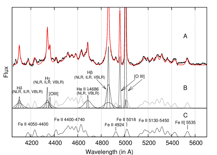
Figure 14: An example of the best fit (date Nov 23, 2001) of the $\lambda\lambda$4000-5600 Å  region: (A) the observed spectra (dots) and the best fit (solid line). (B) H$\beta$, H$\gamma$, and H$\delta$ fit with the sum of three Gaussians representing emission from the NLR, ILR and BLR. The [O III] $\lambda\lambda$4959, 5007 Å lines are fit with two Gaussians for each line of the doublet and He II $\lambda$4686 Å is fit with one broad and one narrow Gaussian. The Fe II template is denoted with a dotted line, and also represented separately in panel (C).

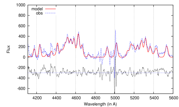
Figure 15: An example of the Fe II line emission (date Nov 23, 2001) in $\lambda\lambda$ 4100-5600 Å  cleared from the contamination of other strong lines in the field. The observed (dashed line) and fitted spectra (solid line) are shown. The bottom line represents the residuals.

An example of a best fit is presented in Fig 14, where all the strong emission lines and Fe II features are labeled. Since the gaussian best-fit includes large number of free parameters (see Fig 14), we focused our attention in the fit required to reproduce as close as possible the Fe II line emission. To this aim, first we fit the strong hydrogen and helium lines, and correct their contribution to the Fe II lines, and then we apply the best-fit procedure to the Fe II emission. With this scheme, we substract the emission of all other lines and deal only with the Fe II spectrum (Fig 15). We fixed as many as possible Gaussian parameters, e.g. the ratio of [OIII] lines, or widths of the Balmer line components NLR, ILR and BLR (ILR - intermidiate-line region, see also Zhang, 2011) The line parameters inferred from our fits (width, shift, intensity relative to total H$\beta$) are given in Table 10.

Kovačević et al. (2010) divided the Fe II emission into subgroups according to the lower level of the transition. We used the same criteria, thus we considered here 6 line groups: ⁴P, ⁴F, ⁶S, ⁴G, ²H, and I Zw 1 line group. In Fig. 16 we plot the fluxes of all these line groups, and the total Fe II emission in the 4100–5600 Å, against the continuum flux at 5100 Å. We omitted the ⁴P group, since below 4200 Å the points are missing for more than 50% of considered spectra, and thus the flux measurements for this group are systematically lower. The total Fe II emission is correlating well with the continuum (r$\sim$0.63, P$<10^{-10}$). This correlation is slightly smaller than the one obtained for the measured Fe II in the wavelength region 5100–5470 Å (see Fig. 11). The Fe ⁴G line group consists of the transitions that contribute the most to the Fe II emission in 5100–5470 Å range, and for this line group we obtained practically the same correlation with the continuum variation as it was measured and presented in Fig. 11 (r$\sim$0.74, P$<10^{-16}$). A relatively good correlations (r$\sim$0.50, P$<10^{-6}$) is obtained for ⁴G group (lines located in the blue part of the Fe II shelf) and for the high-excitation energy group of I Zw 1 (r$\sim$0.56, P$<10^{-8}$), while the other two groups have no correlation at all: Fe ²H (r$\sim$-0.01 and P$=0.82$) and Fe ⁶S (r$\sim$0.14 and P$=0.18$). In the case of Fe ²H this could probably be due the very weak emission coming from these transitions, while in Fe ⁶S it seems to be a real effect.

We compared the width of the Fe II lines to the widths of different H$\beta$ components (Table 10). The average value of the Fe II lines is the same (within the error bars) to the average width value of the ILR component of the H$\beta$ line (Fig. 17). This clearly supports the idea that the origin of the Fe II emission is more within the ILR than the BLR as stated before (see e.g. Marziani & Sulentic, 1993; Popović et al., 2004, 2009; Kovačević et al., 2010).

The quantity R_Fe, defined as the flux ratio of optical Fe II emission to H$\beta$ line, is an important one in describing the EV1 parameter space (see Boroson & Green, 1992). Here the H$\beta$ flux includes the contributions of all three components (narrow, intermidiate and broad), but still represents the behavior of the broad H$\beta$ since the flux of the narrow component is expected to be constant. The variations of R_Fe as a function of the blue continuum flux are plotted in Fig. 18. This plot shows a weak (statistically insignificant), but positive correlation between R_Fe and continuum flux (the correlation coefficient r$\sim$0.36, and P$<10^{-3}$).

6 Discussion

6.1 The structure of the line emitting region in Ark 564

The permitted-line profiles of Ark 564 are Lorentzian like, that can be found in a group of AGNs with FWHM of broad lines smaller than 4000 km s^-1 (Sulentic et al., 2009; Marziani et al., 2010; Sulentic et al., 2011). The problem is, that, such line profiles are not expected in the classical BLR. The Lorentzian-like line profile can be caused by the composition of the three Gaussian profiles (as it was shown in Kovačević et al., 2010), where the contribution of the narrow component is significant. As e.g. Contini et al. (2003) roughly estimated the contribution of the BLR to the total H$\beta$ line and to the permitted lines in the UV and found that H$\beta_{\rm broad}$/H$\beta_{\rm narrow}$ should range between 1 and 2, that is not far from our estimation, that narrow component contributes to the total line flux with $\sim$20%. Also, Rodríguez-Ardila et al. (2000) showed that the flux carried out by the narrow component of H$\beta$ in a sample of seven NLS1s is, on average, 50% of the total line flux. Therefore, such high contribution of the narrow component to the total line flux can bring a small rate of variation in broad lines, and that the emission of the very broad component is very weak, i.e. that a relatively small fraction of the total flux in lines is coming from the BLR.

The observed weak variation in the permitted lines of Ark 564 during a 10-year period is in agreement with a short term monitoring covering 2-year period given by Shemmer et al. (2001), they found no significant optical line variations. It is interesting that there is a weak correlation between the permitted lines and continuum variation. This, as well as the lack of correlation between H$\alpha$ and H$\beta$, may indicate different sources of ionization, as e.g. the shock wave ionization in addition to the photoionization. Moreover, five flare-like events (two prominent and three possible ones) are registered during the monitoring period, that confirm flare-like variability reported in Collier et al. (2001) and indicate burst events in the emission line regions. These may indicate some kind of explosions (in starburst regions) which can additionally affect the line and continuum emission. The small [OIII]/H$\beta_{\rm narrow}$ ratio may also indicate a presence of starbursts in the center of Ark 564 (as it was noted for Mrk 493, see Popović et al., 2009).

Taking into account that it is very hard to properly decompose the narrow component (see discussion in Popović & Kovačević, 2011, in more details) from the broad one, it is hard to discuss about the geometry of the BLR of Ark 564. However, a lack of significant correlation between the H$\alpha$ and H$\beta$ flux variation, may indicate that there is a very stratified (in physical parameters, see Sec. 4.1) emitting region, where the H$\beta$ emitting region tends to be more compact than the H$\alpha$ one. This idea is supported by the detected differences in the FWHM and FW0I of H$\alpha$ and H$\beta$, and the absent correlation between the BD and continuum (Fig. 8). On the other hand, the quasi-simultaneous variations of H$\alpha$ and H$\beta$ blue and red wing (Fig. 6) and their good correlations (Fig. 9) indicate a predominantly circular motions in the BLR.

We calculated the CCF and found the delay of only a couple of days. Taking the H$\beta$ width and lag (assuming that the H$\beta$ lag corresponds to the dimension of the BLR) one can estimate the mass of the black hole of $\sim 1\cdot 10^{6}$ Solar masses, that is in agreement with previous estimates by Shemmer et al. (2001); Collier et al. (2001); Pounds et al. (2001), and also well fit the hypothesis that NLS1s have lower black hole masses than typical Sy1s. However, one should take with caution this estimates, since there is no large correlation between the permitted lines and continuum variability. The CCF may indicate that the variability (perturbation) is coming from relatively small region, but it is interesting that it causes amplification of total line flux without significant change in line profiles (even during flare-like events). The permitted line profiles stay practically the same during the whole monitoring period (see Fig. 7).

6.2 Fe II emission variability in Ark 564

The variability behavior of the Fe II complex in Seyfert galaxies has been poorly understood (see Collin & Joly, 2000). As e.g. Kollatschny et al. (2001) reported that in Mrk 110 the permitted optical Fe II complex remained constant within 10% error over 10 years, while the forbidden [Fe X]$\lambda$6375 line was variable. Similarly, in the Seyfert 1 galaxy NGC 5548 no significant variations of the optical Fe II blends (less than 20%) were detected (Dietrich et al., 1993). However, the opposite result was reported in a long term optical variability watch program on Seyfert 1 galaxy NGC 7603 over a period of nearly 20 years (Kollatschny et al., 2000). This object displayed remarkable variability in the Fe II feature, with amplitudes of the same order as for the H$\alpha$ and He I lines. Giannuzzo & Stripe (1996) found that, out of 12 NLS1s, at least 4 of them presented a significant variability of the Fe II complex with percentage variations larger than 30%. In addition, considerable variations of the Fe II emission (larger than 50%) were reported in two Seyfert 1 galaxies: Akn 120 and Fairall 9 (Kollatschny et al., 1981; Kollatschny & Fricke, 1985). On the other hand Kuehn et al. (2008) performed a reverberation analysis of the strong, variable optical Fe II emission bands in the spectrum of Ark 120 and they were unable to measure a clear reverberation lag for these Fe II lines on any timescale. They concluded that the optical Fe II emission does not come from a photoionization-powered region similar in size to the H$\beta$ emitting region. Our results confirm this since for different groups there are different correlation with the continuum and in some groups (as e.g. ${}^{6}S$) there is no correlation at all (see discussion below).

The most interesting is that the Fe II variation (at least in the red part of Fe II shelfs) in Ark 564 is closely following the variations in the continuum. Similar result was obtained in the case of NGC 4051, an NLS1 galaxy, where the variability of the optical Fe II emission also followed the continuum variability (Wang et al., 2005).

We investigate the time variability of several Fe II multiplets in Ark 564. An interesting result is that there are different levels of correlations between the emission of Fe II line groups and continuum flux. It seems that the level of Fe II flux variability depends on the type of transition. For example, we found the good correlation for ⁴G and ⁴F groups which mainly contribute to the blue and red Fe II features around H$\beta$, and practically no significant correlation between ²H and ⁶S group and continuum (Fig. 13). The emission from these two groups seem to be variable, but there is no respons to the continuum variability. This also may indicate that the Fe II emission region in Ark 564 is stratified. On the other hand, the width of Fe II lines follow the width of the ILR component, that is in a good agreement with results reported in previous work (Marziani & Sulentic, 1993; Popović et al., 2004, 2009; Kovačević et al., 2010)

We found a positive (yet, statistically not significant) trend of R_Fe with the blue continuum. Wang et al. (2005) found the similar positive trend for the galaxy NGC 4051, in opposition to the negative trend observed in NGC 7603 (reported by Wang et al., 2005, on the data of Kollatschny et al. 2000). They argued, by comparing the variability behaviors of different objects, that the objects with positive correlations have narrow H$\beta$ lines and consequently are classified as NLS1s. While the remaining two sources with negative correlations have relatively broad H$\beta$ profiles. They interpreted that the dichotomy in variability behavior of R_Fe is due to the different physical conditions governing the variability of the optical Fe II emission. Our result is consistent with their findings supporting their idea that in case of NLS1 we have that the bulk excitation of the optical Fe II lines is due to collisional excitation in a high density optically thick cloud illuminated and heated mainly by X-rays photons (see Wang et al., 2005, and references therein).

7 Conclusion

In this paper, we analyzed the long spectral variability of NLS1 galaxy Ark 564, observed in the 11-year period from 1999 to 2010. We performed a detail analysis of optical spectra covering the continuum flux at 5100 Å and 6200 Å and H$\beta$, H$\alpha$ and Fe II lines. Here we briefly outline our conclusion:

1) In Ark 564 during the monitoring period (1999–2010) the mean continuum and lines fluxes decreased for $\sim$20%-30% (see Fig. 5) from the beginning (1999) to the end of the monitoring (2010). The total flux of Fe II evidently increases with the continuum flux.

2) We registered five flare-like events (two prominent and three possible) lasting $\sim$1-3 days, when fluxes in continuum and lines changed for $\sim$20% (continuum and Fe II emission) and $\sim$10% for Balmer lines.

3) The flux-flux correlations between the continuum and lines are weak, where the correlation between the Fe II lines (in the red shelf of the Fe II) and continuum is slightly higher (and more significant) than between the Balmer lines and continuum. There is almost lack of correlation between the H$\alpha$ and H$\beta$ line fluxes. Such behavior indicate very complex physical processes in the line forming region, i.e. beside the photoionization some additional physical processes may be present.

4) We roughly estimated a lag of 2–6 days, but with large errorbars. Taking that the photoionization is probably not the only source of line excitation, the obtained results should be taken with caution.

5) We investigated in detail, the Fe II emission variability. We divided the Fe II emission in six groups according to the atomic transitions. We found that correlation between the continuum flux and emission of groups depends on the type of transition, i.e. in some case there is relatively good correlation level between the Fe II group emission (⁴G, ⁴F group), but for ²H and ⁶S there is no correlation at all.

6) The Gaussian multicomponent analysis indicates that the emission of the Fe II lines is probably coming from the intermidiate line region, having velocities around 1500 km/s.

The spectral variability of Ark 564 seems to be complex and different from the one observed in BLS1 (see e.g. Shapovalova et al., 2009). The observed flare-like events, the small (or even lack of) correlation between H$\alpha$ and H$\beta$ fluxes, the different correlation degree for Fe II group emission and continuum light level, may indicate complex physics in the emitting regions, as e.g. there may be, beside the AGN, contribution of star explosions and internal shock waves.

Figure 4: The Fe II emission around the H$\beta$ line for Ark 564.

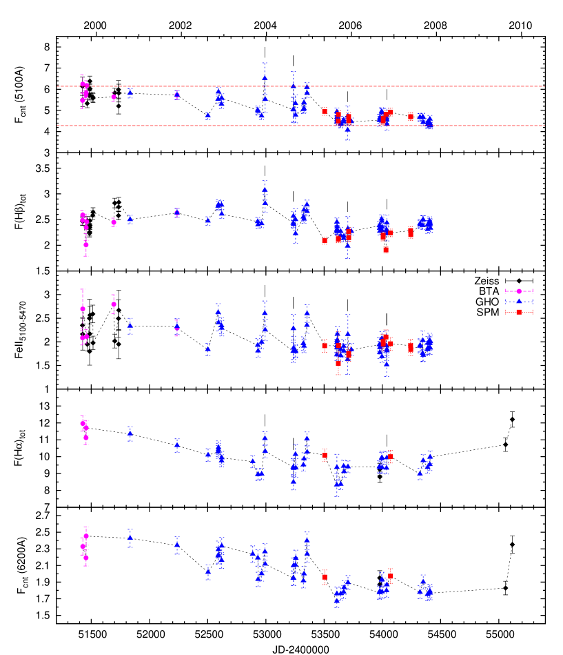
Figure 5: Light curves (from top to the bottom) of the continuum at 5100 Å  H$\beta$, Fe II, H$\alpha$ and the continuum at 6200 Å. Data obtained with different telescopes are marked with different symbols: diamonds - 6m BTA, circles - 1m Zeiss, triangles - 2.1m GHO, squares - 2.1m SPM. The flares are marked on the upper four plot (see Table 6), while in the blue continuum plot (first upper plot) the dashed lines represent the first and last observed continuum flux to show the decrease of the continuum flux during the monitoring campaign. Continuum fluxes are given in units 10${}^{-15}\rm erg\ cm^{-2}s^{-1}$ Å^-1 and line fluxes in 10${}^{-13}\rm erg\ cm^{-2}s^{-1}$.

Figure 6: Light curves of the H$\alpha$ (left) and H$\beta$ (right) line-segments (from top to bottom: blue, core, and red line parts).

Figure 9: H$\alpha$ and H$\beta$ line-wing fluxes (blue, red) vs. line-core flux (upper panels), and red vs. blue-wing (bottom panel). The correlation coefficient and the corresponding P-value are given in the upper left corner.

Figure 10: H$\alpha$ and H$\beta$ line and line-segment fluxes (blue, core and red) vs. continuum flux at 6300 and 5100, respectively. The correlation coefficient and the corresponding P-value are given in the upper left corner.

Figure 11: H$\alpha$ (upper), H$\beta$ (middle), Fe II (bottom) emission against the continuum flux at 5100. The correlation coefficient and the corresponding P-value are given in the upper left corner.

Figure 12: Balmer decrement vs. continuum flux at 5100 Å. The correlation coefficient and the corresponding P-value are given in the upper left corner.

Figure 16: Fe II line fluxes (different groups and total fluxes) vs. continuum flux at 5100 Å. The correlation coefficient and the corresponding p-value are given in the upper left corner.

Figure 17: Gaussian widths of the Fe II lines compared with the widths of the H$\beta$ ILR component. The vertical line shows the average value of Fe II widths, while the horizontal lines show the average values of the H$\beta$ BLR, ILR and NLR components.

Figure 18: R_FeII plotted against the blue continuum flux (EV1 parameter plane).

Table 1: Sources of spectroscopic observations.

Observatory	Code	Tel.aperture + equipment	Aperture	Focus	No.	Period
1	2	3	4	5	6	7
SAO(Russia)	L(U)	6 m + UAGS	2.0$\times$6.0	Prime	9	1999–2001
SAO(Russia)	L(N)	6 m + UAGS	2.0$\times$6.0	Nasmith	1	1999 Oct 09
SAO(Russia)	Z1K	1 m + UAGS+CCD1K	4.0$\times$19.8	Cassegrain	19	1999–2001
SAO(Russia)	Z2K	1 m + UAGS+CCD2K	4.0$\times$4.0	Cassegrain	5	2006–2009
Gullermo Haro (México)	GHO	2.1 m + B&C	2.5$\times$6.0	Cassegrain	74	2000–2007
San–Pedro Martir (México)	SPM	2.1 m + B&C	2.5$\times$6.0	Cassegrain	12	2005–2007

Note. — Col.(1): Observatory. Col.(2): Code assigned to each combination of telescope + equipment used throughout this paper. Col.(3): Telescope aperture and spectrograph. Col.(4): Projected spectrograph entrance apertures (slit width$\times$slit length in arcsec). Col.(5): Focus of the telescope. Col.(6): Number or spectra obtained. Col.(7): Observation period.

Table 2: The log of spectroscopic observations.

N	UT-date	JD+	CODE	Aperture	Sp.range	Res	Seeing
		2400000+		arcsec	Å	Å	arcsec
1	2	3	4	5	6	7	8
1	1999Sep02	51424.4	Z1K	4.0$\times$19.8	4025-5825	7	2.0
2	1999Sep03	51425.4	L(U)	2.0$\times$6.0	3620-6044	9	1.5
3	1999Sep04	51426.4	Z1K	4.0$\times$19.8	4025-5825	7	2.0
4	1999Sep05	51427.3	L(U)	2.0$\times$6.0	3650-6074	8	1.6
5	1999Sep05	51427.4	L(U)	2.0$\times$6.0	4900-7324	9	1.6
6	1999Oct03	51455.2	L(U)	2.0$\times$6.0	4320-5568	5	1.3
7	1999Oct03	51455.3	L(U)	2.0$\times$6.0	6030-7278	5	1.3
8	1999Oct04	51456.2	L(U)	2.0$\times$6.0	4320-5556	6	1.3
9	1999Oct04	51456.3	L(U)	2.0$\times$6.0	6040-7276	5	1.3
10	1999Oct09	51461.3	L(N)	2.0$\times$6.0	4240-6590	8	2.5
11	1999Oct13	51465.2	Z1K	4.0$\times$19.8	4050-5850	6	2.0
12	1999Nov02	51485.3	Z1K	4.0$\times$19.8	4025-5825	7	2.0
13	1999Nov03	51486.2	Z1K	4.0$\times$19.8	4025-5825	7	2.0
14	1999Nov04	51487.2	Z1K	4.0$\times$19.8	4025-5825	6	2.0
15	1999Nov05	51488.2	Z1K	4.0$\times$19.8	4025-5825	8	2.0
16	1999Nov06	51489.2	Z1K	4.0$\times$19.8	4025-5825	7	2.0
17	1999Nov30	51513.2	Z1K	4.0$\times$19.8	4025-5825	7	2.0
18	1999Dec02	51515.2	Z1K	4.0$\times$19.8	4050-5850	8	2.0
19	2000May28	51693.5	L(U)	2.0$\times$6.0	3550-5974	8	1.6
20	2000Jun06	51702.4	Z1K	4.0$\times$19.8	4020-5820	8	3.0
21	2000Jul08	51734.4	Z1K	4.0$\times$19.8	4050-5850	8	3.0
22	2000Jul09	51735.4	Z1K	4.0$\times$19.8	4050-5850	7	3.0
23	2000Jul10	51736.4	Z1K	4.0$\times$19.8	4030-5830	7	3.0
24	2000Oct16	51833.7	GHO	2.5$\times$6.0	4000-7300	12	2.3
25	2001Aug29	52151.5	Z1K	4.0$\times$19.8	4040-5840	7	2.0
26	2001Aug29	52151.5	Z1K	4.0$\times$19.8	5600-7290	8	2.0
27	2001Oct08	52191.2	Z1K	4.0$\times$19.8	4050-5850	8	2.0
28	2001Oct09	52192.3	Z1K	4.0$\times$19.8	4040-5840	7	2.0
29	2001Oct09	52192.4	Z1K	4.0$\times$19.8	5640-7290	11	2.0
30	2001Nov23	52237.1	L(U)	2.0$\times$6.0	3600-6024	10	3.5
31	2001Nov23	52236.6	GHO	2.5$\times$6.0	4200-5960	8	2.5
32	2001Nov24	52237.6	GHO	2.5$\times$6.0	6000-7360	9	1.5
33	2002Aug15	52501.8	GHO	2.5$\times$6.0	4270-5840	10	2.5
34	2002Aug17	52503.9	GHO	2.5$\times$6.0	5700-7460	10	2.0
35	2002Nov11	52589.7	GHO	2.5$\times$6.0	4300-6060	8	4.5
36	2002Nov12	52590.7	GHO	2.5$\times$6.0	5700-7460	10	2.7
37	2002Nov13	52591.7	GHO	2.5$\times$6.0	5700-7460	9	2.7
38	2002Nov14	52592.7	GHO	2.5$\times$6.0	3800-7100	10	2.7
39	2002Dec10	52618.6	GHO	2.5$\times$6.0	4300-6060	8	1.5
40	2002Dec11	52619.6	GHO	2.5$\times$6.0	5700-7460	9	1.8
41	2002Dec12	52620.6	GHO	2.5$\times$6.0	3800-7100	13	1.8
42	2003Sep04	52886.9	GHO	2.5$\times$6.0	5700-7460	11	2.3
43	2003Oct17	52929.7	GHO	2.5$\times$6.0	4300-6060	10	2.3
44	2003Oct18	52930.7	GHO	2.5$\times$6.0	5700-7460	11	1.8
45	2003Oct20	52932.7	GHO	2.5$\times$6.0	3800-7100	12	1.8
46	2003Nov19	52962.6	GHO	2.5$\times$6.0	4300-6060	10	2.3
47	2003Nov20	52963.7	GHO	2.5$\times$6.0	5700-7460	12	2.6
48	2003Dec17	52990.6	GHO	2.5$\times$6.0	4300-6060	9	3.1
49	2003Dec18	52991.6	GHO	2.5$\times$6.0	5300-7460	12	2.7
50	2003Dec20	52993.6	GHO	2.5$\times$6.0	3800-7100	15	2.3
51	2004Aug17	53234.9	GHO	2.5$\times$6.0	3800-7100	15	2.5
52	2004Aug18	53235.8	GHO	2.5$\times$6.0	4300-6060	9	3.1
53	2004Aug19	53236.8	GHO	2.5$\times$6.0	5700-7460	12	3.1
54	2004Aug20	53237.9	GHO	2.5$\times$6.0	3800-7100	15	2.7
55	2004Sep05	53253.9	GHO	2.5$\times$6.0	3800-7100	15	2.7
56	2004Sep06	53254.8	GHO	2.5$\times$6.0	4300-6060	8	2.7
57	2004Sep08	53256.8	GHO	2.5$\times$6.0	5700-7460	10	3.6
58	2004Nov12	53321.6	GHO	2.5$\times$6.0	3800-7100	14	2.3
59	2004Nov17	53326.6	GHO	2.5$\times$6.0	4300-6060	11	2.7
60	2004Nov18	53327.6	GHO	2.5$\times$6.0	3800-7100	14	2.3
61	2004Dec13	53352.6	GHO	2.5$\times$6.0	3800-7100	12	3.6
62	2004Dec14	53353.6	GHO	2.5$\times$6.0	4300-6060	7	3.6
63	2004Dec15	53354.6	GHO	2.5$\times$6.0	5700-7460	8	2.3
64	2005May14	53505.0	SPM	2.5$\times$6.0	3880-5960	7	4.9
65	2005May15	53506.0	SPM	2.5$\times$6.0	5720-7580	7	3.3
66	2005Aug26	53608.9	GHO	2.5$\times$6.0	3800-7100	13	2.9
67	2005Aug27	53609.9	GHO	2.5$\times$6.0	4150-7460	12	3.4
68	2005Aug28	53610.8	GHO	2.5$\times$6.0	4330-6000	7	2.8
69	2005Aug29	53611.8	GHO	2.5$\times$6.0	4330-6000	8	3.9
70	2005Aug30	53612.8	GHO	2.5$\times$6.0	4330-6000	8	3.3
71	2005Aug31	53613.8	GHO	2.5$\times$6.0	4330-6000	7	2.7
72	2005Sep08	53621.9	SPM	2.5$\times$6.0	3700-5790	10	3.0
73	2005Sep09	53622.9	SPM	2.5$\times$6.0	3700-5780	8	-
74	2005Sep28	53641.8	GHO	2.5$\times$6.0	4320-5980	7	2.7
75	2005Sep29	53642.6	GHO	2.5$\times$6.0	5740-7400	8	3.1
76	2005Sep30	53643.8	GHO	2.5$\times$6.0	4290-5960	7	2.8
77	2005Oct24	53667.6	GHO	2.5$\times$6.0	3750-7050	12	2.3
78	2005Oct26	53669.7	GHO	2.5$\times$6.0	4260-5920	8	3.0
79	2005Oct28	53671.7	GHO	2.5$\times$6.0	5740-7400	8	3.1
80	2005Nov28	53702.6	GHO	2.5$\times$6.0	3800-6908	14	3.0
81	2005Nov29	53703.6	GHO	2.5$\times$6.0	4300-5917	8	5.0
82	2005Nov30	53704.6	GHO	2.5$\times$6.0	5740-7400	8	2.0
83	2005Dec05	53710.6	SPM	2.5$\times$6.0	3700-5770	7	-
84	2005Dec07	53711.6	SPM	2.5$\times$6.0	3700-5770	7	2.8
85	2005Dec29	53733.6	GHO	2.5$\times$6.0	4300-6010	10	2.3
86	2006Jun28	53915.5	Z2K	4.0$\times$4.0	3740-7400	9	2.5
87	2006Aug27	53974.9	GHO	2.5$\times$6.0	3600-7050	12	2.2
88	2006Aug29	53977.5	Z2K	4.0$\times$4.0	3750-7400	9	2.0
89	2006Aug30	53978.5	Z2K	4.0$\times$4.0	3750-7400	8	2.0
90	2006Aug30	53977.8	GHO	2.5$\times$6.0	4120-5920	8	2.5
91	2006Aug31	53978.8	GHO	2.5$\times$6.0	3600-7050	12	2.2
92	2006Sep15	53993.8	GHO	2.5$\times$6.0	3600-7050	13	3.4
93	2006Sep17	53995.7	GHO	2.5$\times$6.0	3600-7050	13	2.4
94	2006Sep18	53996.8	GHO	2.5$\times$6.0	4130-5030	7	2.5
95	2006Sep19	53997.8	GHO	2.5$\times$6.0	3600-7000	12	2.8
96	2006Sep28	54006.7	SPM	2.5$\times$6.0	3740-5810	7	3.3
97	2006Sep29	54007.7	SPM	2.5$\times$6.0	3740-5810	7	3.3
98	2006Oct23	54031.7	SPM	2.5$\times$6.0	3700-5900	8	2.6
99	2006Oct27	54035.7	GHO	2.5$\times$6.0	3700-7280	12	2.8
100	2006Oct28	54036.7	GHO	2.5$\times$6.0	4230-6040	8	2.4
101	2006Oct30	54038.7	GHO	2.5$\times$6.0	3700-7270	14	2.3
102	2006Oct31	54039.7	GHO	2.5$\times$6.0	4160-5960	8	2.3
103	2006Nov30	54069.6	SPM	2.5$\times$6.0	3680-7560	12	4.6
104	2007May22	54242.9	SPM	2.5$\times$6.0	3730-5810	8	3.0
105	2007May23	54244.0	SPM	2.5$\times$6.0	3730-5810	8	3.2
106	2007Aug10	54322.9	GHO	2.5$\times$6.0	3870-7430	11	3.0
107	2007Aug11	54323.8	GHO	2.5$\times$6.0	4340-6140	7	3.2
108	2007Sep03	54346.8	GHO	2.5$\times$6.0	4330-6130	7	3.6
109	2007Sep04	54347.8	GHO	2.5$\times$6.0	4150-5950	7	2.6
110	2007Sep07	54350.9	GHO	2.5$\times$6.0	3860-7420	12	3.0
111	2007Oct15	54388.7	GHO	2.5$\times$6.0	3870-7440	12	1.8
112	2007Oct17	54390.6	GHO	2.5$\times$6.0	4190-6000	8	2.5
113	2007Oct18	54391.7	GHO	2.5$\times$6.0	4190-6000	8	2.2
114	2007Nov01	54405.7	GHO	2.5$\times$6.0	4190-6000	8	3.0
115	2007Nov02	54406.6	GHO	2.5$\times$6.0	4190-6000	8	3.3
116	2007Nov03	54407.6	GHO	2.5$\times$6.0	3820-7390	12	2.9
117	2007Nov06	54410.7	GHO	2.5$\times$6.0	3830-7400	12	2.4
118	2007Nov08	54412.6	GHO	2.5$\times$6.0	4290-6100	8	2.4
119	2009Aug14	55058.5	Z2K	4.0$\times$4.0	3750-7390	8	2.0
120	2009Oct11	55116.4	Z2K	4.0$\times$4.0	3750-7390	8	1.5

Note. — Col.(1): Number. Col.(2): UT date. Col.(3): Julian date (JD). Col.(4): CODE. Col.(5): Projected spectrograph entrance apertures. Col.(6): Wavelength range covered. Col.(7): Spectral resolution. Col.(8): Mean seeing in arcsec.

Table 3: Flux scale factors for optical spectra.

Sample	Years	Aperture	Scale factor	Extended source correction
		(arcsec)	($\varphi$)	G(g)
L(U,N)	1999–2010	2.0$\times$6.0	1.089	-0.130
GHO	1999–2007	2.5$\times$6.0	1.000	0.000
SPM	2005–2007	2.5$\times$6.0	1.000	0.000
Z1K	1999–2001	4.0$\times$19.8	1.152$\pm$0.013	0.998$\pm$0.368
Z2K	2005–2007	4.0$\times$4.0	0.893$\pm$0.052	1.005$\pm$0.548
GHO	1999–2007	2.5$\times$6.0	1.067$\pm$0.048	0.000

Table 4: The measured line and continuum fluxes.

N	UT-date	JD+	F${}_{\rm cnt}\pm\sigma$	F(H$\alpha$)$\pm\sigma$	F(H$\beta$)$\pm\sigma$	Fe II${}_{5100-5470}\pm\sigma$
		2400000+	$10^{-15}\rm erg\,cm^{-2}s^{-1}$Å-1	$10^{-13}\rm erg\,cm^{-2}s^{-1}$	$10^{-13}\rm erg\,cm^{-2}s^{-1}$	$10^{-13}\rm erg\,cm^{-2}s^{-1}$
1	2	3	4	5	6	7
1	1999Sep02	51424.4	6.145$\pm$ 0.430	-	2.471 $\pm$ 0.082	2.349$\pm$ 0.170
2	1999Sep03	51425.4	5.479$\pm$ 0.384	-	2.486 $\pm$ 0.082	2.085$\pm$ 0.151
3	1999Sep04	51426.4	5.507$\pm$ 0.325	-	2.464 $\pm$ 0.081	2.162$\pm$ 0.336
4	1999Sep05	51427.3	6.246$\pm$ 0.437	11.963$\pm$ 0.447	2.589 $\pm$ 0.085	2.696$\pm$ 0.419
5	1999Oct03	51455.2	5.733$\pm$ 0.214	11.119$\pm$ 0.416	2.008 $\pm$ 0.221	-
6	1999Oct04	51456.2	5.828$\pm$ 0.218	11.707$\pm$ 0.438	2.348 $\pm$ 0.258	-
7	1999Oct09	51461.3	6.176$\pm$ 0.231	-	2.459 $\pm$ 0.081	2.111$\pm$ 0.152
8	1999Oct13	51465.2	5.329$\pm$ 0.199	-	2.478 $\pm$ 0.082	1.948$\pm$ 0.141
9	1999Nov02	51485.3	5.742$\pm$ 0.215	-	2.233 $\pm$ 0.074	2.496$\pm$ 0.405
10	1999Nov03	51486.2	5.705$\pm$ 0.213	-	2.253 $\pm$ 0.074	1.798$\pm$ 0.291
11	1999Nov04	51487.2	6.013$\pm$ 0.225	-	2.348 $\pm$ 0.077	2.170$\pm$ 0.352
12	1999Nov05	51488.2	6.384$\pm$ 0.239	-	2.478 $\pm$ 0.082	-
13	1999Nov06	51489.2	6.030$\pm$ 0.226	-	2.388 $\pm$ 0.079	2.566$\pm$ 0.185
14	1999Nov30	51513.2	5.635$\pm$ 0.211	-	2.584 $\pm$ 0.085	2.590$\pm$ 0.187
15	1999Dec02	51515.2	5.583$\pm$ 0.209	-	2.643 $\pm$ 0.087	1.978$\pm$ 0.143
16	2000May28	51693.5	5.643$\pm$ 0.211	-	2.447 $\pm$ 0.081	2.794$\pm$ 0.202
17	2000Jun06	51702.4	5.829$\pm$ 0.218	-	2.822 $\pm$ 0.093	2.016$\pm$ 0.146
18	2000Jul08	51734.4	5.982$\pm$ 0.431	-	2.578 $\pm$ 0.085	2.493$\pm$ 0.394
19	2000Jul09	51735.4	5.208$\pm$ 0.375	-	2.745 $\pm$ 0.091	1.950$\pm$ 0.308
20	2000Jul10	51736.4	5.822$\pm$ 0.419	-	2.836 $\pm$ 0.094	2.669$\pm$ 0.422
21	2000Oct16	51833.7	5.809$\pm$ 0.217	11.346$\pm$ 0.424	2.500 $\pm$ 0.083	2.330$\pm$ 0.168
22	2001Nov23	52236.6	5.722$\pm$ 0.214	-	2.630 $\pm$ 0.087	2.292$\pm$ 0.168
23	2001Nov23	52237.1	5.725$\pm$ 0.214	-	2.629 $\pm$ 0.087	2.324$\pm$ 0.166
24	2001Nov24	52237.6	-	10.658$\pm$ 0.399	-	-
25	2002Aug15	52501.8	4.747$\pm$ 0.178	-	2.472 $\pm$ 0.082	1.836$\pm$ 0.133
26	2002Aug17	52503.9	-	10.094$\pm$ 0.378	-	-
27	2002Nov11	52589.7	5.528$\pm$ 0.207	-	2.760 $\pm$ 0.091	2.619$\pm$ 0.189
28	2002Nov12	52590.7	-	10.285$\pm$ 0.385	-	-
29	2002Nov13	52591.7	-	10.402$\pm$ 0.389	-	-
30	2002Nov14	52592.7	5.873$\pm$ 0.220	10.537$\pm$ 0.394	2.790 $\pm$ 0.092	2.403$\pm$ 0.173
31	2002Dec10	52618.6	5.294$\pm$ 0.198	-	2.782 $\pm$ 0.092	2.341$\pm$ 0.169
32	2002Dec11	52619.6	-	9.750$\pm$ 0.365	-	-
33	2002Dec12	52620.6	5.578$\pm$ 0.209	9.936$\pm$ 0.372	2.607 $\pm$ 0.086	2.288$\pm$ 0.165
34	2003Sep04	52886.9	-	9.700$\pm$ 0.363	-	-
35	2003Oct17	52929.7	5.016$\pm$ 0.188	-	2.460 $\pm$ 0.081	1.928$\pm$ 0.139
36	2003Oct18	52930.7	-	8.925$\pm$ 0.334	-	-
37	2003Oct20	52932.7	4.961$\pm$ 0.186	8.950$\pm$ 0.335	2.398 $\pm$ 0.079	1.807$\pm$ 0.130
38	2003Nov19	52962.6	4.738$\pm$ 0.177	-	2.420 $\pm$ 0.080	1.993$\pm$ 0.144
39	2003Nov20	52963.7	-	8.968$\pm$ 0.335	-	-
40	2003Dec17	52990.6	6.504$\pm$ 0.748	-	3.070 $\pm$ 0.190	2.600$\pm$ 0.264
41	2003Dec18	52991.6	-	11.069$\pm$ 0.414	-	-
42	2003Dec20	52993.6	5.526$\pm$ 0.636	10.313$\pm$ 0.386	2.813 $\pm$ 0.174	2.251$\pm$ 0.229
43	2004Aug17	53234.9	5.038$\pm$ 0.589	9.375$\pm$ 0.506	2.429 $\pm$ 0.080	1.798$\pm$ 0.235
44	2004Aug18	53235.8	6.123$\pm$ 0.716	-	2.566 $\pm$ 0.085	2.280$\pm$ 0.298
45	2004Aug19	53236.8	-	8.489$\pm$ 0.458	-	-
46	2004Aug20	53237.9	5.027$\pm$ 0.588	9.303$\pm$ 0.502	2.405 $\pm$ 0.079	1.872$\pm$ 0.245
47	2004Sep05	53253.9	5.325$\pm$ 0.405	10.132$\pm$ 0.598	2.501 $\pm$ 0.208	1.812$\pm$ 0.131
48	2004Sep06	53254.8	4.781$\pm$ 0.363	-	2.225 $\pm$ 0.185	1.793$\pm$ 0.129
49	2004Sep08	53256.8	-	9.327$\pm$ 0.550	-	-
50	2004Nov12	53321.6	5.046$\pm$ 0.189	9.504$\pm$ 0.355	2.548 $\pm$ 0.084	1.964$\pm$ 0.142
51	2004Nov17	53326.6	5.369$\pm$ 0.201	-	2.687 $\pm$ 0.089	-
52	2004Nov18	53327.6	5.085$\pm$ 0.190	9.862$\pm$ 0.369	2.508 $\pm$ 0.083	1.909$\pm$ 0.138
53	2004Dec13	53352.6	6.088$\pm$ 0.228	11.049$\pm$ 0.413	2.787 $\pm$ 0.092	2.350$\pm$ 0.170
54	2004Dec14	53353.6	5.814$\pm$ 0.217	-	2.657 $\pm$ 0.088	2.596$\pm$ 0.187
55	2004Dec15	53354.6	-	10.268$\pm$ 0.384	-	-
56	2005May14	53505.0	4.954$\pm$ 0.185	-	2.091 $\pm$ 0.069	1.918$\pm$ 0.138
57	2005May14	53506.0	-	10.081$\pm$ 0.377	-	-
58	2005Aug26	53608.9	4.448$\pm$ 0.166	8.321$\pm$ 0.691	2.283 $\pm$ 0.075	1.919$\pm$ 0.139
59	2005Aug27	53609.9	4.937$\pm$ 0.185	9.362$\pm$ 0.777	2.450 $\pm$ 0.081	1.724$\pm$ 0.125
60	2005Aug28	53610.8	4.559$\pm$ 0.170	-	2.310 $\pm$ 0.076	1.988$\pm$ 0.144
61	2005Aug29	53611.8	4.678$\pm$ 0.175	-	2.360 $\pm$ 0.078	1.880$\pm$ 0.136
62	2005Aug30	53612.8	4.593$\pm$ 0.172	-	2.268 $\pm$ 0.075	2.035$\pm$ 0.147
63	2005Aug31	53613.8	4.704$\pm$ 0.176	-	2.289 $\pm$ 0.076	2.160$\pm$ 0.156
64	2005Sep08	53621.9	4.498$\pm$ 0.168	-	2.118 $\pm$ 0.070	1.543$\pm$ 0.238
65	2005Sep09	53622.9	4.809$\pm$ 0.180	-	2.128 $\pm$ 0.070	1.921$\pm$ 0.296
66	2005Sep28	53641.8	4.333$\pm$ 0.162	-	2.270 $\pm$ 0.075	1.708$\pm$ 0.123
67	2005Sep29	53642.6	-	8.359$\pm$ 0.313	-	-
68	2005Sep30	53643.8	4.378$\pm$ 0.164	-	2.182 $\pm$ 0.072	1.838$\pm$ 0.133
69	2005Oct24	53667.6	4.556$\pm$ 0.170	9.429$\pm$ 0.353	2.133 $\pm$ 0.070	1.908$\pm$ 0.138
70	2005Oct26	53669.7	4.457$\pm$ 0.167	-	2.176 $\pm$ 0.072	1.806$\pm$ 0.130
71	2005Oct28	53671.7	-	9.112$\pm$ 0.341	-	-
72	2005Nov28	53702.6	4.072$\pm$ 0.470	-	1.982 $\pm$ 0.239	1.628$\pm$ 0.321
73	2005Nov29	53703.6	4.736$\pm$ 0.470	-	2.320 $\pm$ 0.239	2.156$\pm$ 0.425
74	2005Nov30	53704.6	-	9.397$\pm$0.351	-	-
75	2005Dec05	53710.6	4.714$\pm$ 0.176	-	2.267 $\pm$ 0.075	1.761$\pm$ 0.127
76	2005Dec07	53711.6	4.507$\pm$ 0.169	-	2.146 $\pm$ 0.071	1.714$\pm$ 0.124
77	2005Dec29	53733.6	4.475$\pm$ 0.167	-	2.270 $\pm$ 0.075	1.834$\pm$ 0.132
78	2006Aug27	53974.9	4.538$\pm$ 0.286	9.399$\pm$ 0.352	2.384 $\pm$ 0.079	1.942$\pm$ 0.140
79	2006Aug29	53977.5	-	9.254$\pm$ 0.346	-	-
80	2006Aug30	53977.8	4.642$\pm$ 0.174	-	2.335 $\pm$ 0.077	1.774$\pm$ 0.128
81	2006Aug30	53978.5	-	8.801$\pm$ 0.329	-	-
82	2006Aug31	53978.8	4.558$\pm$ 0.170	9.337$\pm$ 0.349	2.273 $\pm$ 0.075	1.877$\pm$ 0.135
83	2006Sep15	53993.8	4.953$\pm$ 0.185	9.883$\pm$ 0.370	2.511 $\pm$ 0.083	1.959$\pm$ 0.141
84	2006Sep17	53995.7	4.889$\pm$ 0.183	9.941$\pm$ 0.372	2.469 $\pm$ 0.081	2.068$\pm$ 0.149
85	2006Sep18	53996.8	4.899$\pm$ 0.183	-	2.288 $\pm$ 0.076	1.686$\pm$ 0.122
86	2006Sep19	53997.8	4.626$\pm$ 0.173	9.352$\pm$ 0.350	2.352 $\pm$ 0.078	1.916$\pm$ 0.138
87	2006Sep28	54006.7	4.501$\pm$ 0.168	-	2.156 $\pm$ 0.071	2.011$\pm$ 0.145
88	2006Sep29	54007.7	4.625$\pm$ 0.173	-	2.200 $\pm$ 0.073	1.951$\pm$ 0.141
89	2006Oct23	54031.7	4.819$\pm$ 0.180	-	1.910 $\pm$ 0.063	2.101$\pm$ 0.152
90	2006Oct27	54035.7	4.643$\pm$ 0.174	9.319$\pm$ 0.349	2.305 $\pm$ 0.076	1.916$\pm$ 0.317
91	2006Oct28	54036.7	4.570$\pm$ 0.171	-	2.280 $\pm$ 0.075	1.515$\pm$ 0.250
92	2006Oct30	54038.7	4.781$\pm$ 0.320	9.930$\pm$ 0.371	2.434 $\pm$ 0.153	1.840$\pm$ 0.133
93	2006Oct31	54039.7	4.348$\pm$ 0.291	-	2.225 $\pm$ 0.141	1.810$\pm$ 0.131
94	2006Nov30	54069.6	4.922$\pm$ 0.184	9.999$\pm$ 0.374	2.240 $\pm$ 0.074	1.959$\pm$ 0.141
95	2007May22	54242.9	4.702$\pm$ 0.176	-	2.285 $\pm$ 0.075	1.919$\pm$ 0.139
96	2007May23	54244.0	4.707$\pm$ 0.176	-	2.209 $\pm$ 0.073	1.839$\pm$ 0.133
97	2007Aug10	54322.9	4.683$\pm$ 0.175	8.973$\pm$ 0.336	2.398 $\pm$ 0.079	1.907$\pm$ 0.138
98	2007Aug11	54323.8	4.667$\pm$ 0.175	-	2.422 $\pm$ 0.080	1.927$\pm$ 0.139
99	2007Sep03	54346.8	4.668$\pm$ 0.175	-	2.491 $\pm$ 0.082	1.758$\pm$ 0.177
100	2007Sep04	54347.8	4.696$\pm$ 0.176	-	2.385 $\pm$ 0.079	2.027$\pm$ 0.204
101	2007Sep07	54350.9	4.430$\pm$ 0.166	9.760$\pm$ 0.365	2.496 $\pm$ 0.082	1.715$\pm$ 0.124
102	2007Oct15	54388.7	4.318$\pm$ 0.161	9.360$\pm$ 0.350	2.306 $\pm$ 0.076	1.834$\pm$ 0.132
103	2007Oct17	54390.6	4.446$\pm$ 0.166	-	2.401 $\pm$ 0.079	1.969$\pm$ 0.142
104	2007Oct18	54391.7	4.344$\pm$ 0.162	-	2.396 $\pm$ 0.079	1.874$\pm$ 0.135
105	2007Nov01	54405.7	4.413$\pm$ 0.165	-	2.403 $\pm$ 0.079	2.033$\pm$ 0.147
106	2007Nov02	54406.6	4.399$\pm$ 0.165	-	2.472 $\pm$ 0.082	1.871$\pm$ 0.135
107	2007Nov03	54407.6	4.594$\pm$ 0.172	9.530$\pm$ 0.356	2.444 $\pm$ 0.081	1.964$\pm$ 0.142
108	2007Oct06	54410.7	4.367$\pm$ 0.163	9.973$\pm$ 0.373	2.414 $\pm$ 0.080	1.870$\pm$ 0.135
109	2007Nov08	54412.6	4.287$\pm$ 0.160	-	2.332 $\pm$ 0.077	2.002$\pm$ 0.145
110	2009Aug14	55058.5	-	10.712$\pm$ 0.401	-	-
111	2009Oct11	55116.4	-	12.204$\pm$ 0.456	-	-

Table 5: Estimates of the errors for line and line-segment fluxes.

Line	Spectral Region		$\sigma\pm$e	$V_{r}$ region
	[Å] (obs)	[Å] (rest)	[%]	km s-1
cont 5100	5220–5250	5094–5123	3.7 $\pm$3.3	-
cont 6200	6320–6370	6168–6216	4.5 $\pm$2.2	-
H$\alpha$ - total	6640–6810	6480–6646	3.7 $\pm$2.2	(-3792;+3792)
H$\beta$ - total	4936–5030	4817–4909	3.3 $\pm$2.5	(-2710;+2950)
Fe II	5226–5605	5100–5470	7.2 $\pm$5.6	-
H$\alpha$ - blue	6635–6698	6475–6537	6.8 $\pm$6.6	(-4015;-1204)
H$\alpha$ - core	6698–6752	6537–6589	3.5 $\pm$2.1	(-1204;+1204)
H$\alpha$ - red	6752–6816	6589–6652	5.6 $\pm$4.0	(+1204;+4015)
H$\beta$ - blue	4928–4960	4809–4840	8.0 $\pm$4.9	(-3200;-1200)
H$\beta$ - core	4960–5001	4840–4880	3.0 $\pm$2.9	(-1200;+1200)
H$\beta$ - red	5001–5034	4880–4913	8.7 $\pm$5.3	(+1200;+3200)

Table 6: Flares in light curves of the blue continuum, H$\beta$, H$\alpha$, and Fe II emission.

N	DATE	JD+	F(cnt)	dF(cnt)	F(H$\beta$)	dF(H$\beta$)	F(H$\alpha$)	dF(H$\alpha$)	F(Fe II)	dF(Fe II)
		2400000	(5235)Å	%		%		%		%
1	2003Dec17	52990.6	6.5038	18%	3.070	9%	11.069	7%	2.600	10%
	2003Dec20	52993.6	5.5264		2.813		10.313		2.251
2	2004Aug17	53234.9	5.0378	22%	2.429	6%	9.375	10%	1.798	13%
	2004Aug18	53235.8	6.1232		2.566		8.489		2.280
	2004Aug20	53237.9	5.0271		2.405		9.303		1.872
3	2005Nov28	53702.6	4.0724	16%	1.982	17%	-	-	1.628	20%
	2005Nov29	53703.6	4.7362		2.320		-		2.156
4	2006Oct27	54035.7							1.916	17%
	2006Oct28	54036.7							1.515
5	2006Oct30	54038.7	4.7813	10%	2.434	9%	9.319	7%	1.840	7%
	2006Oct31	54039.7	4.3478		2.225		9.930		1.810

Table 7: Parameters of the continuum and line variabilities.

Feature	N	Region [Å]	$F$(mean)	$\sigma$($F$)	$R$(max/min)	$F$(var)
1	2	3	4	5	6	7
continuum 5100	91	5094–5123	5.068	0.608	1.597	0.107
continuum 6300	50	6168–6216	2.021	0.218	1.471	0.098
H$\alpha$ - total	50	6480–6646	9.856	0.878	1.467	0.079
H$\beta$ - total	91	4817–4909	2.413	0.206	1.607	0.075
Fe II	87	5100–5470	2.029	0.280	1.844	0.096
H$\alpha$ - blue	50	6475–6537	0.652	0.079	1.852	0.081
H$\alpha$ - core	50	6537–6589	8.581	0.757	1.445	0.080
H$\alpha$ - red	50	6589–6652	0.731	0.074	1.605	0.077
H$\beta$ - blue	91	4809–4840	0.220	0.040	3.465	0.149
H$\beta$ - core	91	4840–4880	2.008	0.152	1.566	0.064
H$\beta$ - red	91	4880–4913	0.258	0.040	2.238	0.110

Note. — Col.(1): Analyzed feature of the spectrum. Col.(2): Total number of spectra. Col.(3): Wavelength region (in the rest frame). Col.(4): Mean flux. Col.(5): Standard deviation. Col.(6): Ratio of the maximal to minimal flux . Col.(7): Variation amplitude (see text).

Table 8: Lags and CCF between the continuum and lines.

LC1-LC2	lag (days)	CCF
cnt-H$\beta$tot	3.56${}^{+27.44}_{3.56}$	0.49${}^{+0.08}_{-0.09}$
cnt-Fe II	0.02${}^{+2.02}_{2.08}$	0.52${}^{+0.08}_{-0.08}$
cnt-H$\alpha$tot	4.54${}^{+5.54}_{14.46}$	0.49${}^{+0.01}_{-0.01}$

Table 9: Line transitions added to the Fe II template given in Tables 1 and 2 of Kovačević et al. (2010). The atomic data are taken from the NIST atomic database.

Fe II multiplet	Transition	Wavelength [Å]
Fe II 27-28	b4P5/2 – z4F${}_{3/2}^{o}$	4087.284
	b4P5/2 – z4F${}_{5/2}^{o}$	4122.668
	b4P5/2 – z4D${}_{3/2}^{o}$	4128.748
	b4P5/2 – z4D${}_{5/2}^{o}$	4173.461
	b4P5/2 – z4F${}_{7/2}^{o}$	4178.862
	b4P5/2 – z4D${}_{7/2}^{o}$	4233.172
	b4P3/2 – z4F${}_{3/2}^{o}$	4258.154
	b4P3/2 – z4D${}_{1/2}^{o}$	4273.326
	b4P3/2 – z4F${}_{5/2}^{o}$	4296.572
	b4P3/2 – z4D${}_{3/2}^{o}$	4303.176
	b4P3/2 – z4D${}_{5/2}^{o}$	4351.769
	b4P1/2 – z4F${}_{3/2}^{o}$	4369.411
	b4P1/2 – z4D${}_{1/2}^{o}$	4385.387
	b4P1/2 – z4D${}_{3/2}^{o}$	4416.830
	b4P5/2 – z6F${}_{7/2}^{o}$	4670.182
Fe II] 55	b2H9/2 – z4D${}_{7/2}^{o}$	5525.125
	b2H11/2 – z4F${}_{9/2}^{o}$	5534.847

Table 10: The line parameters (w-widths, s-shifts, i-intensity) from the gaussian best-fitting of H$\beta$ and Fe II lines for 91 good-resolution spectra.

JD+	w NLR	s NLR	i NLR	w ILR	s ILR	i ILR	w BLR	s BLR	i BLR	w Fe II	s Fe II	i Fe II
2400000+	km/s	km/s	[%]	km/s	km/s	[%]	km/s	km/s	[%]	km/s	km/s	[%]
1	2	3	4	5	6	7	8	9	10	11	12	13
51424.4	525	36	0.21	1843	0	0.35	5493	0	0.44	1699	77	1.98
51425.4	504	20	0.20	1712	0	0.53	6238	-90	0.27	1627	6	1.90
51426.4	429	21	0.18	1534	0	0.48	5491	390	0.33	1347	125	1.62
51427.3	429	21	0.15	1538	0	0.48	5488	150	0.37	1694	19	2.30
51455.2	349	24	0.19	1578	0	0.60	5491	150	0.21	1602	3	2.14
51456.2	346	24	0.17	1443	30	0.54	6021	148	0.29	1398	56	1.55
51461.3	429	21	0.21	1560	0	0.57	3994	240	0.22	1450	-24	2.04
51465.2	409	15	0.17	1446	0	0.45	4995	-240	0.38	1497	-25	1.98
51485.3	409	15	0.16	1498	150	0.43	4992	0	0.41	1498	93	2.36
51486.2	409	15	0.15	1248	30	0.42	5241	90	0.43	1547	0	2.26
51487.2	409	15	0.16	1248	30	0.43	4992	0	0.41	1448	0	1.72
51488.2	409	15	0.16	1447	30	0.43	5491	0	0.41	1448	174	2.19
51489.2	409	15	0.15	1348	30	0.45	5491	0	0.40	1498	0	2.06
51513.2	409	15	0.15	1348	30	0.43	5491	0	0.42	1497	-22	2.26
51515.2	409	15	0.14	1348	30	0.41	5990	-450	0.44	1448	0	1.75
51693.5	410	101	0.16	1349	30	0.46	5489	300	0.39	1446	79	2.00
51702.4	449	30	0.15	1348	30	0.39	4992	0	0.46	1398	267	1.60
51734.4	450	30	0.17	1349	30	0.44	4998	-1	0.39	1499	173	2.27
51735.4	444	30	0.14	1348	30	0.36	5491	0	0.51	1547	0	2.43
51736.4	444	30	0.13	1298	30	0.33	5492	0	0.54	1547	180	2.03
51833.7	593	5	0.16	1548	-6	0.46	4968	0	0.37	1552	-66	1.97
52237.1	699	0	0.20	1467	60	0.45	5001	0	0.35	1714	21	2.14
52236.6	499	0	0.19	1548	0	0.42	4991	-30	0.39	1598	26	1.76
52501.8	540	15	0.19	1548	0	0.48	4992	-30	0.33	1497	-133	1.67
52589.7	474	0	0.19	1548	0	0.42	5492	-30	0.39	1497	17	1.75
52592.7	599	-42	0.14	1503	-101	0.45	5621	-98	0.40	1736	0	1.85
52618.6	444	18	0.20	1529	-41	0.48	4893	-33	0.33	1494	48	1.68
52620.6	700	1	0.17	1548	0	0.38	5490	-30	0.45	1647	1	2.16
52929.7	534	9	0.19	1454	31	0.40	4714	28	0.40	1539	12	1.77
52932.7	703	1	0.21	1549	0	0.46	4492	0	0.33	1597	41	1.92
52962.6	524	0	0.20	1448	30	0.41	4493	30	0.39	1547	-59	1.71
52990.6	500	15	0.21	1448	30	0.47	3993	30	0.32	1446	56	1.78
52993.6	849	30	0.21	1547	30	0.40	4993	60	0.39	1597	46	1.81
53234.9	749	27	0.21	1448	0	0.41	4743	0	0.37	1498	-49	1.84
53235.8	499	15	0.18	1447	30	0.43	4742	0	0.39	1448	-2	1.88
53237.9	749	27	0.20	1447	0	0.42	4795	15	0.38	1497	-29	1.95
53253.9	764	27	0.21	1443	-6	0.41	4840	20	0.38	1490	-34	1.84
53254.8	414	18	0.15	1260	30	0.44	4993	0	0.41	1647	14	1.77
53321.6	749	27	0.20	1448	0	0.43	4791	15	0.37	1498	-7	1.76
53326.6	599	15	0.20	1448	30	0.42	4742	0	0.38	1448	135	1.65
53327.6	749	27	0.18	1448	0	0.42	4793	15	0.40	1498	23	1.77
53352.6	649	27	0.18	1548	-60	0.41	4793	15	0.42	1597	-57	1.87
53353.6	499	15	0.20	1448	0	0.42	4741	0	0.38	1448	62	1.94
53495.0	397	15	0.18	1398	15	0.46	4986	16	0.36	1498	52	2.12
53608.9	699	0	0.21	1497	0	0.42	4742	15	0.36	1597	-44	2.11
53609.9	699	0	0.21	1498	0	0.42	4742	15	0.37	1597	3	1.90
53610.8	400	17	0.16	1347	0	0.46	4991	15	0.38	1548	-22	1.70
53611.8	404	24	0.16	1353	-1	0.45	4886	16	0.38	1518	-59	1.64
53612.8	433	19	0.17	1325	-6	0.43	5048	-34	0.40	1505	-92	1.62
53613.8	399	0	0.16	1332	-27	0.44	5091	15	0.40	1548	-90	1.64
53620.9	465	-14	0.17	1337	-60	0.43	5091	15	0.40	1497	-134	1.83
53622.9	464	-15	0.18	1278	0	0.42	4992	15	0.40	1498	2	1.86
53641.8	419	15	0.19	1278	0	0.42	4992	15	0.39	1498	-71	1.52
53643.8	414	22	0.16	1225	30	0.46	4992	0	0.39	1648	-19	1.76
53667.6	699	0	0.21	1497	0	0.42	4742	15	0.36	1597	-87	1.92
53669.7	419	0	0.17	1278	0	0.40	4991	15	0.42	1497	-5	1.81
53702.6	699	3	0.19	1298	0	0.40	4991	0	0.41	1498	-67	1.85
53703.6	449	12	0.19	1298	0	0.44	4992	0	0.37	1498	61	1.81
53710.6	364	12	0.15	1248	0	0.42	4991	15	0.43	1498	-20	1.80
53711.6	364	12	0.15	1248	0	0.42	4992	15	0.43	1497	0	1.80
53733.6	449	12	0.16	1248	0	0.47	4393	60	0.37	1498	-119	1.69
53974.9	649	0	0.19	1498	0	0.46	4742	15	0.35	1598	-67	1.84
53977.8	399	12	0.15	1248	0	0.40	5491	-300	0.44	1498	-9	1.62
53978.8	649	0	0.19	1498	0	0.46	4743	15	0.35	1597	-37	1.87
53993.8	650	0	0.19	1497	0	0.46	4746	15	0.36	1598	-67	1.87
53995.7	650	15	0.19	1497	0	0.46	4741	15	0.35	1598	-92	1.90
53996.8	415	18	0.16	1263	30	0.43	4985	0	0.41	1601	-7	1.73
53997.8	639	15	0.19	1472	0	0.45	4742	15	0.36	1597	-75	1.84
54006.7	364	12	0.17	1248	0	0.48	4492	300	0.35	1397	19	1.90
54007.7	364	12	0.18	1247	0	0.48	4493	300	0.34	1397	6	1.83
54031.7	369	60	0.19	1148	90	0.43	4492	300	0.38	1398	248	2.01
54035.7	639	15	0.19	1473	0	0.45	4742	15	0.36	1597	-90	1.85
54036.7	405	20	0.18	1298	0	0.42	4992	0	0.40	1398	-8	1.58
54038.7	725	1	0.20	1470	0	0.44	4740	15	0.36	1600	-85	1.85
54039.7	401	3	0.16	1296	0	0.42	5001	-1	0.42	1399	-84	1.79
54069.6	599	0	0.19	1448	30	0.45	4743	15	0.37	1597	-57	2.07
54242.9	400	3	0.18	1297	0	0.42	5088	0	0.41	1450	8	1.92
54244.0	399	3	0.20	1298	0	0.45	4842	0	0.35	1447	-16	1.91
54322.9	604	0	0.20	1446	30	0.46	4740	15	0.35	1598	-26	1.86
54323.8	414	18	0.17	1306	30	0.43	4992	0	0.39	1547	-1	1.49
54346.8	399	3	0.20	1298	0	0.44	4493	0	0.36	1448	-6	1.63
54347.8	399	3	0.19	1298	0	0.41	4493	0	0.40	1447	-2	2.07
54350.9	606	0	0.21	1460	29	0.46	4488	14	0.33	1596	-65	1.77
54388.7	599	15	0.19	1448	30	0.47	4493	15	0.34	1598	-100	1.85
54390.6	400	3	0.20	1298	0	0.43	4243	150	0.37	1448	15	1.91
54391.7	399	3	0.18	1298	0	0.43	4493	150	0.40	1448	25	1.88
54405.7	399	3	0.18	1298	0	0.43	4493	150	0.39	1447	-15	1.86
54406.6	399	3	0.18	1298	0	0.43	4493	150	0.39	1448	-22	1.85
54407.6	599	15	0.21	1448	30	0.45	4493	15	0.34	1597	-49	2.01
54410.7	607	14	0.20	1451	30	0.45	4495	16	0.35	1595	-71	1.95
54412.6	399	3	0.17	1297	0	0.40	4993	0	0.42	1448	3	1.80
mean	507$\pm$128	13$\pm$16	0.18$\pm$0.02	1404$\pm$120	9$\pm$28	0.44$\pm$0.04	4938$\pm$405	25$\pm$109	0.38$\pm$0.05	1523$\pm$81	-2$\pm$74	1.87$\pm$0.19

References

- Alexander (1997) Alexander, T. 1997, Astronomical Time Series, ed. D. Maoz, A. Sternberg, & E. M. Leibowitz (Dordrecht: Kluwer), 163
- Bischoff & Kollatschny (1999) Bischoff, K., & Kollatschny, W. 1999, A&A, 345, 49B
- Boller et al. (1996) Boller, Th., Brandt, W. N., Fink, H. 1996, A&A, 305, 53
- Boroson & Green (1992) Boroson, T. A., & Green, R. F. 1992, ApJS, 80, 109
- Chiho et al. (2004) Chiho, M., Karen M. L., Herman L. M. 2004, ApJ, 603, 456
- Crenshaw et al. (1999) Crenshaw, D. M., Kraemer, S. B., Boggess, A., Maran, S. P., Mushotzky, R. F., Wu, C.-C. 1999, ApJ, 516, 750
- Crenshaw et al. (2002) Crenshaw, D. M., Kraemer, S. B., Turner, T. J., et al. 2002, ApJ, 566, 187
- Cruise & Dodds (1985) Cruise, A. M., & Dodds, P. M. 1985, MNRAS, 215, 417
- Collier et al. (2001) Collier, S., Crenshaw, D. M., Peterson, B. M. et al. 2001, 561, 146
- Collin & Joly (2000) Collin, S., Joly, M. 2000, NewAR, 44, 531
- Contini et al. (2003) Contini, M., Rodríguez-Ardila, A., Viegas, S. M. 2003, A&A, 408, 101
- de Vaucouleurs et al. (1991) De Vaucouleurs, G., De Vaucouleurs, A., Corwin, H. G. Jr., et al. 1991, in Third Reference Catalogue of Bright Galaxies (New York: Springer-Verlag)
- Dietrich et al. (1993) Dietrich, M., Kollatschny, W., Peterson, B. M., et al. 1993, ApJ, 408, 416
- Hufnagel & Bregman (1992) Hufnagel, B. R., & Bregman, J. N. 1992, ApJ, 386, 473
- Hughes et al. (1992) Hughes, P. A., Aller, H. D., Aller, M. F. 1992, ApJ, 396, 469
- Giannuzzo & Stripe (1996) Giannuzzo, E. M., Stirpe, G. M. 1996, A&A, 314, 419
- Ilić et al. (2012) Ilić, D., Popović, L. Č., La Mura, G., Ciroi, S., Rafanelli, P. 2012, A&A, accepted (eprint arXiv:1205.3950)
- Kollatschny et al. (2000) Kollatschny, W., Bischoff, K., Dietrich, M. 2000, A&A, 361, 901
- Kollatschny et al. (2001) Kollatschny, W., Bischoff, K., Robinson, E. L., Welsh, W. F., Hill, G. J. 2001, A&A, 379, 125
- Kollatschny & Fricke (1985) Kollatschny, W., Fricke, K. J. 1985, A&A, 146, L11
- Kollatschny et al. (1981) Kollatschny, W., Schleicher, H., Fricke, K. J., Yorke, H. W. 1981, A&A, 104, 198
- Kovačević et al. (2010) Kovačević, J., Popović, L. Č., Dimitrijević, M. S. 2010, ApJS, 189, 15
- Kuehn et al. (2008) Kuehn, C. A., Baldwin, J. A., Peterson, B. M., Korista, K. T. 2008, ApJ, 673, 69
- Kuraszkiewicz et al. (2002) Kuraszkiewicz, J. K., Green, P. J., Forster, K., Aldcroft, T. L., Evans, I. N., Koratkar, A. 2002, ApJS, 143, 257
- Leighly (1999a) Leighly, K. M. 1999a, ApJS, 125, 297
- Leighly (1999b) Leighly, K. M. 1999b, ApJS, 125, 317
- Leighly (2000) Leighly, K. M. 2000, NewAR, 44, 395
- Marziani & Sulentic (1993) Marziani, P., Sulentic, J. W. 1993, ApJ, 558, 553
- Marziani et al. (2010) Marziani, P., Sulentic, J. W., Negrete, C. A., Dultzin, D., Zamfir, S., Bachev, R. 2010, MNRAS, 409, 1033
- O’Brien et al. (1998) O’Brien P.T., Dietrich, M., Leighly, K et al. 1998, ApJ, 509, 163
- Osterbrock & Pogge (1985) Osterbrock, D. E., Pogge, R. W. 1985, ApJ, 297, 166
- Panessa et al. (2011) Panessa, F., de Rosa, A., Bassani, L., Bazzano, A., Bird, A., Landi, R., Malizia, A., Miniutti, G., Molina, M., Ubertini, P. 2011, MNRAS, 417, 2426
- Peterson (1993) Peterson B. M., 1993, PASP105, 207
- Peterson et al. (1999) Peterson, B. M., Barth, A. J., Berlind, P. et al. 1999, ApJ, 510, 659
- Peterson et al. (1994) Peterson, B. M., Berlind, P., Bertram, R. et al. 1994, ApJ, 425, 622
- Peterson et al. (2002) Peterson, B. M., Berlind, P., Bertram, R. et al. 2002, ApJ. 581, 197
- Peterson & Collins (1983) Peterson, B. M., & Collins, G. W., II 1983, ApJ, 270, 71
- Peterson et al. (1995) Peterson, B. M., Pogge, R.W., Wanders, I., Smith, S. M., Romanishin, W. 1995, PASP, 107, 579
- Popović & Kovačević (2011) Popović, L. Č., Kovačević, J. 2011, ApJ, 738, 68
- Popović et al. (2004) Popović, L. Č., Mediavilla, E., Bon, E., Ilić, D. 2004, A&A, 423, 909
- Popović et al. (2009) Popović, L. Č., Smirnova, A., Kovačević, J., Moiseev, A., Afanasiev, V. 2009, AJ, 137, 3548
- Pounds et al. (2001) Pounds, K., Edelson, R., Markowitz, A., Vaughan, S. 2001, ApJ, 550, 15
- Rodríguez-Ardila et al. (2000) Rodríguez-Ardila, A., Pastoriza, M. G., Binette, L., & Donzelli, C. J. 2000, ApJ, 538, 581
- Shapovalova et al. (2004) Shapovalova, A. I., Doroshenko, V. T., Bochkarev, N. G. et al. 2004, A&A, 422, 925
- Shapovalova et al. (2008) Shapovalova, A. I., Popović, L. Č., Collin, S., Burenkov, A. N., Chavushyan, V. H., Bochkarev, N. G., Benítez, E., Dultzin, D., Kovačević, A., Borisov, N., Carrasco, L., León-Tavares, J., Mercado, A., Valdes, J. R., Vlasuyk, V. V., Zhdanova, V. E. 2008, A&A, 486, 99
- Shapovalova et al. (2009) Shapovalova, A. I., Popović, L. Č., Bochkarev, N. G., Burenkov, A. N., Chavushyan, V. H., Collin, S., Doroshenko, V. T., Ilić, D., Kovačević, A. 2009, NewAR, 53, 191.
- Shapovalova et al. (2010) Shapovalova, A. I., Popović, L. Č., Chavushyan, V. H., et al. 2010, A&A517, id.A42
- Shemmer et al. (2001) Shemmer, O., Romano, P., Bertram, R. et al. 2001, ApJ, 561, 162
- Smith et al. (2008) Smith, R. A. N.; Page, M. J.; Branduardi-Raymont, G. 2008, ApJ, 490, 103
- Sulentic et al. (2007) Sulentic, J. W., Bachev, R., Marziani, P., Negrete, C. A., Dultzin, D. 2007, ApJ, 666, 757
- Sulentic et al. (2009) Sulentic, J., Marziani, P., Zamfir, S. 2009, NewAR, 53, 198
- Sulentic et al. (2011) Sulentic, J., Marziani, P., Zamfir, S. 2011, BaltA, 20, 427
- Turner et al. (2001) Turner, T. J., Romano, P., George, I. M., Edelson, R., Collier, S. J., Mathur, S., Peterson, B. M. 2001, ApJ, 561, 131
- Van Groningen & Wanders (1992) Van Groningen, E. & Wanders, I. 1992, PASP, 104, 700
- Wang et al. (2005) Wang, J., Wei, J. Y., He, X. T.2005, A&A, 436, 417
- Zhang (2011) Zhang, X.-G. 2005, ApJ, 741, 104