CERN-PH-TH/2012-193  NORDITA-2012-54

Loop corrections and a new test of inflation

Abstract

Inflation is the leading paradigm for explaining the origin of primordial density perturbations. However many open questions remain, in particular whether one or more scalar fields were present during inflation and how they contributed to the primordial density perturbation. We propose a new observational test of whether multiple fields, or only one (not necessarily the inflaton) generated the perturbations. We show that our test, relating the bispectrum and trispectrum, is protected against loop corrections at all orders, unlike previous relations.

Introduction: The statistical distribution of the primordial density field provides a unique opportunity to test our understanding of the origin of the observed Universe. Inflation is the leading paradigm, but many questions about its details remain and it is so flexible that it is unclear if it can ever be ruled out. However it is at least possible to test, in a model independent way, whether a single source present during inflation was responsible for generating density perturbations, or whether multiple sources are required, by exploiting deviations from a Gaussian distribution. Non-Gaussianity (nonG) parameters are related by distinctive consistency relations, whose structure generally depends on whether perturbations are produced by one or more scalar fields. These parameters could be measured by forthcoming Planck satellite data and we may be able to answer fundamental questions about the number of degrees of freedom contributing to the primordial density perturbation.

In single-source scenarios, density perturbations are generated by quantum fluctuations in a single scalar field, that does not necessarily correspond to an inflaton field driving the Hubble expansion. Single-field inflation is one particular case of this set-up, in which a single inflaton field both drives inflation and generates primordial cosmological perturbations. More generally, we include also set-ups such as curvaton or modulated reheating scenarios, in the limit that only one field generates the density perturbation Suyama:2010uj . In these models, large nonG of local shape is induced by a single light scalar field, whose dynamics is important on super Hubble scales.

One famous consistency relation associates the squeezed limit of 3-point function with the scale dependence of the 2-point function: $f_{\rm NL}=-\nicefrac{{5}}{{12}}\,(n_{\zeta}-1)$. This relation is valid only for single-field (clock) inflation Creminelli:2004yq , and is violated in more general single-source, or multiple-source scenarios. Another consistency relation, on which we will focus, connects the collapsed limit of 4-point function to the squeezed limit of the 3-point function:

$$\tau_{\rm NL}=\left(\nicefrac{{6f_{\rm NL}}}{{5}}\right)^{2}\,.$$ (1)

This equality is satisfied at tree-level in single-source scenarios (up to gravitational corrections that can violate it by a small amount Seery:2008ax , see however our Conclusions), but is generally violated in multiple-source set-ups, leading to the Suyama-Yamaguchi inequality $\tau_{\rm NL}\geq\left(\nicefrac{{6f_{\rm NL}}}{{5}}\right)^{2}$ Suyama:2007bg ; Smith:2011if ; Assassi:2012zq ; Kehagias:2012pd . Recently it was shown that the equality (1) can be broken at an observable level, even in single-source scenarios, due to loop corrections Byrnes:2011ri ; Sugiyama:2012tr . A popular model which can realise this possibility is the interacting curvaton scenario, several other models also exist Byrnes:2011ri .

Inflationary observables associated with any given $n$-point ($n$-pt) function receive loop contributions, in terms of integrals over internal soft momenta that induce logarithmic corrections proportional to parameters related with higher $n$-pt functions. These contributions are clearly seen in a diagrammatic representation of $n$-pt functions in terms of Feynman-type diagrams Byrnes:2007tm . Loop corrections to correlation functions contribute to $f_{\rm NL}$ and $\tau_{\rm NL}$, and in single-source scenarios, these corrections can combine in such a way to break the equality (1). As we will discuss, the violation of (1) can be interpreted as due to the fact that the equality written in this way does not include contributions of soft momentum lines, connecting different $n$-pt functions entering the definitions of $\tau_{\rm NL}$ and $f_{\rm NL}^{2}$. These soft momentum lines are allowed by momentum conservation, and lead to radiative corrections comparable to the conventional loop corrections. Accounting for both loop corrections and soft modes, we will build a new combination of bispectrum, trispectrum and power spectrum, that leads to an equality satisfied to all orders in radiative corrections in generic single-source scenarios. The equality reduces to equation (1) at tree-level, and is in general broken in multiple-field scenarios. Our result therefore generalizes the Suyama-Yamaguchi relation to all orders in radiative corrections. Moreover, in the second part, we will also discuss how the soft modes we consider are the source of the inhomogeneity of nonG observables discussed in Byrnes:2011ri , leading to further observational implications for our findings. Finally, in the conclusions we will point out that our generalized inequality is preserved by gravitational corrections that spoil (1).

The role of soft momenta is reminiscent of what happens in QED, in which a careful inclusion of contributions of both real and virtual soft photons is crucial for canceling IR divergences in physical processes Bloch:1937pw . The conceptual idea we develop here is similar to what happens in that context, although the technical implementation will be different.

Radiative corrections to $n$-pt functions. From now on we focus on a local Ansatz for the primordial curvature perturbation Wands:2010af

$$\zeta({\bf x})=\zeta_{G}({\bf x})+\frac{3\bar{f}_{\rm NL}}{5}\zeta_{G}^{2}({\bf x})+\frac{9\bar{g}_{\rm NL}}{25}\zeta_{G}^{3}({\bf x})+\frac{81\bar{h}_{\rm NL}}{125}\zeta_{G}^{4}({\bf x})+\cdots-\langle\zeta({\bf x})\rangle\ ,$$ (2)

where $\zeta_{G}$ is a Gaussian random fluctuation, with vanishing ensemble average $\langle\zeta_{G}\rangle\,=\,0$. The local Ansatz assumes the parameters $\bar{f}_{\rm NL}$, $\bar{g}_{\rm NL}$ and $\bar{h}_{\rm NL}$ to be constant. For our arguments, we will assume that these parameters are sufficiently large to be observable: in this case, slow-roll suppressed contributions to non-Gaussianity, associated with the intrinsic non-Gaussianity of the fields under consideration, provide only small corrections to our results in the relevant momentum limits, and can be neglected. We focus on single-source scenarios, in which the curvature perturbation is generated by a single scalar $\sigma$ and with observably large nonG. It is then possible to rewrite the local Ansatz (2) in terms of an expansion of a suitable classical function $N(\sigma)$,

$$\zeta({\bf x}) = N(\sigma_{0}+\delta\sigma({\bf x}))-\langle N(\sigma_{0}+\delta\sigma({\bf x}))\rangle\,=\,\sum_{n=1}^{\infty}\frac{N^{(n)}(\sigma_{0})}{n!}\,\left(\delta\sigma({\bf x})^{n}-\langle\delta\sigma({\bf x})^{n}\rangle\right)$$ (3)

This expansion is similar to the $\delta N$ approach of Lyth:2005fi but for our purposes it is not necessary to specify $N(\sigma)$ further. $\sigma_{0}$ denotes a homogeneous, time dependent background solution and the fluctuations $\delta\sigma({\bf x})$ are Gaussian with zero mean. Making the identification $N^{\prime}(\sigma_{0})\delta\sigma({\bf x})\,=\,\zeta_{G}({\bf x})$, a comparison of the equations (2) and (3) yields the relations $\nicefrac{{6\bar{f}_{\rm NL}}}{{5}}\,=\,\nicefrac{{N^{\prime\prime}}}{{N^{\prime 2}}}$, $\nicefrac{{54\bar{g}_{\rm NL}}}{{25}}\,=\,\nicefrac{{N^{\prime\prime\prime}}}{{N^{\prime 3}}}$, etc Lyth:2005fi .

The general definitions for the parameters $f_{\rm NL}$ and $\tau_{\rm NL}$ at tree-level and beyond are given in appropriate squeezed and collapsed limits by

$${f}_{{\rm NL}} \equiv \frac{5}{12}\,\lim_{k_{1}\to 0}\frac{B(k_{1},k_{2},k_{3})}{P(k_{1})P(k_{2})}\ ,$$ (4)

$${\tau}_{{\rm NL}} \equiv \frac{1}{4}\,\lim_{{k_{12}}\to 0}\frac{T(k_{1},k_{2},k_{3},k_{4},k_{12},k_{13})}{P(k_{12})P(k_{1})P(k_{3})}\ ,$$ (5)

where $\langle\zeta_{{\bf k}_{1}}\zeta_{{\bf k}_{2}}\rangle=(2\pi)^{3}P\delta({\bf k}_{1}+{\bf k}_{2})$, $\langle\zeta_{{\bf k}_{1}}\zeta_{{\bf k}_{2}}\zeta_{{\bf k}_{3}}\rangle\,=\,(2\pi)^{3}B\delta({\bf k}_{1}+{\bf k}_{2}+{\bf k}_{3})$, $\langle\zeta_{{\bf k}_{1}}\zeta_{{\bf k}_{2}}\zeta_{{\bf k}_{3}}\zeta_{{\bf k}_{4}}\rangle\,=\,(2\pi)^{3}T\delta({\bf k}_{1}+{\bf k}_{2}+{\bf k}_{3}+{\bf k}_{4})$, and $k_{ij}=|{\bf k}_{i}+{\bf k}_{j}|$. Notice that at tree-level $f_{\rm NL}$ defined by equation (4) reduces to the parameter $\bar{f}_{\rm NL}$ entering the local Ansatz (2). At tree level one has $\bar{f}_{{\rm NL}}\,=\,\nicefrac{{5\,N^{\prime\prime}}}{{6\,N^{\prime}{}^{2}}}$, $\bar{\tau}_{{\rm NL}}\,=\,\nicefrac{{N^{\prime\prime 2}}}{{N^{\prime}{}^{4}}}$, from which equality (1) follows immediately. Let us stress that, in this work, we focus on the case in which the tree-level bar quantities are constant and do not depend on momenta. However, when 1-loop contributions are added to the tree-level results, one finds

$$f_{\rm NL}^{\rm loop} = \bar{f}_{\rm NL}-\frac{18}{25}\left(2\bar{f}_{\rm NL}^{3}-3\bar{f}_{\rm NL}\bar{g}_{\rm NL}-3\bar{h}_{\rm NL}\right)\,\bar{{\cal P}}\ln{\left(\frac{k}{k_{IR}}\right)}\ ,$$ (6)

$$\tau_{\rm NL}^{\rm loop} = \bar{\tau}_{\rm NL}-\frac{324}{625}\left(8\bar{f}_{\rm NL}^{4}-12\bar{f}_{\rm NL}^{2}g_{\rm NL}-9\bar{g}_{\rm NL}^{2}-12\bar{h}_{\rm NL}\bar{f}_{\rm NL}\right)\,\bar{{\cal P}}\ln{\left(\frac{k}{k_{IR}}\right)},$$

where $2\pi^{2}{\cal P}=k^{3}P(k)$, and we neglect its weak scale dependence. Hence

$$\tau_{\rm NL}^{\rm loop}\,=\,\left(\frac{6f_{\rm NL}^{\rm loop}}{5}\right)^{2}\,\left[1+\frac{81\,\bar{g}_{\rm NL}^{\,2}}{25\bar{f}_{\rm NL}^{\,2}\rule{0.0pt}{9.47217pt}}\,\bar{\cal P}\ln{\left(\frac{k}{k_{IR}}\right)}\right]$$ (7)

showing that the consistency relation (1) is violated already at one loop in single-source models, if the tree-level $\bar{g}_{\rm NL}$ is non-vanishing. More precisely, the consistency relation holds only on the scale $k_{\rm IR}$ at which the tree-level quantities are defined and the loops are absent. Moving away from this scale, the loop corrections become non-zero leading to a violation of the consistency relation. If the nonG parameters are large, this violation of the consistency relation can be observed by the Planck satellite. As a representative example, assume $\bar{f}_{\rm NL}\,=\,20$, and $\bar{g}_{\rm NL}\,=\,8\,\cdot\,10^{5}$, close to the upper bound set by WMAP. See e.g. Enqvist:2008gk for explicit examples of models that theoretically under control, and that can lead to such a large hierarchy between tree level values of $\bar{f}_{\rm NL}$ and $\bar{g}_{\rm NL}$. Without including loop corrections (the square parenthesis in (7)) one would find $\tau_{\rm NL}\,=\,576$: too small value to be observed in the near future, since the forecasted Planck constraint is $\tau_{\rm NL}\gtrsim 1500$ at 1-sigma error bar, in absence of detection Smidt:2010ra (see also Kogo:2006kh for an analysis suggesting that CMB data might lead to even lower values for the detectability of $\tau_{\rm NL}$). Including loops, instead, the value of $\tau_{\rm NL}$ becomes large enough to be detectable: $\tau_{\rm NL}\,\sim\,3600$ setting $\bar{\cal P}\sim 10^{-9}$ to match COBE normalization, and assuming $\ln\left(\nicefrac{{k}}{{k_{IR}}}\right)$ of order one. Hence in this situation loop corrections can really make the difference and render $\tau_{\rm NL}$ detectable even in the single source case.

A couple of considerations on to the physical validity of our calculations. One might be worried with respect to the fact that, choosing such a large value for $\bar{g}_{\rm NL}$ as in the example above, the loop contribution to some $n$-point functions dominate over the tree level term: in particular the third order term in (2) can be larger than the second order term. This raises questions on whether our calculation is under control at the technical level, in particular whether a perturbative approach makes sense. Fortunately it does (provided that terms beyond $\bar{g}_{\rm NL}$ in (2) do not grow too rapidly). Indeed, it is possible to show that only one non-linearity parameter can be associated with each external line in a loop diagram Byrnes:2007tm , and so for the power spectrum the largest possible power of $\bar{g}_{\rm NL}$ is $\bar{g}_{\rm NL}^{2}$ (in general for an $n$-point function it is $\bar{g}_{\rm NL}^{n}$). For the example we consider, this implies that the one-loop term always dominates over higher loops: higher loops to the trispectrum contain at most four powers of of $\bar{g}_{\rm NL}$ but they are also suppressed by higher powers of $\bar{\cal P}$ than the one-loop term in such a way that the total value is smaller. To be specific, there is a 3 loop contribution to $\tau_{\rm NL}$ which goes like $\bar{g}_{\rm NL}^{4}\bar{\cal P}^{3}$, and so although $\bar{g}_{\rm NL}^{2}\bar{\cal P}\gtrsim 1$ one has $\bar{g}_{\rm NL}^{2}\bar{\cal P}^{2}\ll 1$ and hence the one loop term dominates.

A second concern is about the fact that, in the particular case of pure single field inflation, it has been shown that loop corrections can be absorbed in a redefinition of background quantities, by a proper choice of physical coordinates: see Gerstenlauer:2011ti ; Giddings:2011zd ; Giddings:2010nc for the first papers on these topics. More in particular, the basic idea is the following: since field perturbations are necessarily adiabatic in single field inflation, they span the direction of the homogeneous, classical inflationary trajectory. It can be shown that, by means of a change of coordinates, a suitable shift on this background trajectory can be made such to compensate the effects of loop corrections to observable quantities. This fact is however true only for pure single field inflation, and does not apply in our more general context of single source models that lead to large nonG. In this case, indeed, isocurvature fluctuations span directions perpendicular to the homogeneous one, and consequently the corresponding loop effects can not be re-adsorbed by any background redefinition. Hence, the loop effects that we are considering in this paper are fully physical and well defined.

On the other hand, while being well-defined and consistent, the standard way of calculating loop corrections individually to the power spectrum, bispectrum and trispectrum, and then taking appropriate ratios to define the non-linearity parameters beyond tree-level, can miss important physical contributions. Indeed, these loop corrected quantities correctly characterize the ratios of individually measured bispectrum, or trispectrum, and power spectrum. However, when simultaneously measuring combinations of $n$-pt functions, such as the ratios in (4) and (5), one should allow for the inclusion of soft lines connecting distinct $n$-pt functions. Although momentum is of course conserved, no detector is sensitive enough to probe these soft lines: their contribution is physical and must be included. This observation suggests that, besides considering the relation (1), by including the effects of soft modes it is possible to build a new observable combination of $n$-pt functions that leads to an equality protected against radiative corrections. See also Giddings:2011zd for the slow-roll suppressed effect of soft modes on the power spectrum in single clock inflation.

Diagrammatic approach to loop corrections. It is illuminating to discuss the role of soft modes diagrammatically, first in a simple example, and then applying our observations to equality (1). We implement the diagrammatic approach of Byrnes:2007tm . We use solid dots to mark external momenta ${\bf k}_{i}$, with the number of attached propagators to each vertex (corresponding to $P$) giving the number of derivatives of the function $N$, defined by equation (3), associated to the vertex. There are no internal vertices since we assume that $\delta\sigma$ is Gaussian. The numerical factors are the total for each diagram relative to the tree-level term (which may have some possible permutations), and are given by the numerical factor of the given diagram ($\nicefrac{{1}}{{2}}$ if a dressed vertex, otherwise unity at one loop or tree-level), times the number of distinct ways in which the loop can be drawn onto the tree-level diagram.

Let us illustrate the role of soft modes, by considering radiative corrections to the square of the power spectrum as an example. We denote with $(\dots)_{\rm rad}$ the sum of tree-level and radiative contributions to a given quantity. Figure 1 depicts diagrammatically the difference between $(P)_{\rm rad}^{2}$, associated with the observable $\langle\zeta({\bf k})\zeta({\bf k}^{\prime})\rangle^{2}$, and $(P^{2})_{\rm rad}$, denoting another observable, $\langle\zeta^{2}({\bf k})\zeta^{2}({\bf k}^{\prime})\rangle$.

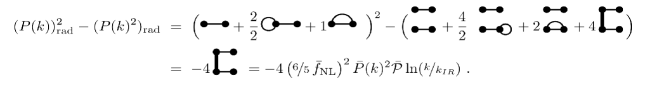
Figure 1: The difference between observables $(P(k))_{\rm rad}^{2}$ and $(P(k)^{2})_{\rm rad}$

The final diagram represents a 4-pt function with a soft internal line (drawn thicker) connecting two $N^{\prime\prime}$ vertices (which can be done in four ways). This contribution cannot be distinguished from the product of two disconnected 2-pt functions and must be included in $(P^{2})_{\rm rad}$. So, accounting for loop corrections only, would not give the correct result for the observable $(P^{2})_{\rm rad}$ , showing the importance of the soft modes.

Contributions to radiative corrections associated with soft lines connecting different diagrams play a crucial role for characterizing equality (1) beyond tree-level. In order to analyze it diagrammatically, it is convenient to re-express it in terms of square of the bispectrum, and the product of the trispectrum with the power spectrum. At tree-level, (1) reads $\bar{B}^{2}_{\,\,k_{1}\rightarrow 0}\,=\,\bar{T}\bar{P}(k_{5})_{\,\,k_{12}\rightarrow 0,\,k_{5}\rightarrow 0}$, where here and in what follows, to avoid ambiguities, we assume that, in the zero momentum limit, all soft momenta coincide: $k_{1}=k_{12}=k_{5}\to 0$. Including loop corrections to $P$, $B$ and $T$, in appropriate squeezed and collapsed limits, the relation is

$$(B)_{\rm rad}^{2}-(P)_{\rm rad}(T)_{\rm rad}\,=\,-4\left(\nicefrac{{54}}{{25}}\,\bar{g}_{\rm NL}\right)^{2}\bar{P}(k)^{2}\bar{P}_{q\rightarrow 0}^{2}\bar{{\cal P}}\ln(\nicefrac{{k}}{{k_{IR}}})\ \,.$$ (8)

So, the equality is broken by a term proportional to tree-level $\bar{g}_{NL}$, as discussed in the previous section. However, a straightforward calculation shows that the relation

$$(B^{2})^{\rm rad}_{k_{1}\to 0} = (PT)^{\rm rad}_{k_{12}\to 0,\,k_{5}\to 0}$$ (9)

$$= \bar{B}^{2}_{\,\,k_{1}\rightarrow 0}\Big{[}1+\left(\nicefrac{{6}}{{5}}\right)^{2}\Big{(}\nicefrac{{3\bar{h}_{\rm NL}}}{{\bar{f}_{\rm NL}}}+\nicefrac{{9\bar{g}_{\rm NL}^{2}}}{{4\bar{f}_{\rm NL}^{2}}}+15\bar{g}_{\rm NL}+6\bar{f}_{\rm NL}^{2}\Big{)}{\bar{\cal P}}\ln(\nicefrac{{k}}{{k_{IR}}})\Big{]}\ ,$$

instead leads to an equality that is preserved by radiative corrections. This new equality holds with for models leading to large nonG of local type, as the ones on which we are focussing our attention in this paper. We have neglected all non-local contributions associated to eventual non-Gaussianity present at horizon crossing. Assuming canonical kinetic terms, this is well justified as the neglected contributions are slow roll suppressed. In the first line of eq. (9), we send to zero a momentum line (denoted with $k_{1}$) in each of the bispectra in the left hand side; in the right hand side, we send to zero the internal momentum line of the trispectrum denoted with $k_{12}$, as well as the momentum $k_{5}$ characterizing the power spectrum. As explained above, all these momenta are made vanishing with the same rate, and coincide in the zero momentum limit. When evaluating the previous quantities, it is crucial to include diagrams describing contributions of soft modes connecting different elements of each combination (drawn thickly in the diagrams below), respectively the 3 diagrams for $(B^{2})_{\rm rad}$ and 2 for $(PT)_{\rm rad}$.

The three first diagrams are 6pt functions consisting of two 3-pt functions connected by a soft line. Analogously to the case of 2-pt function in Fig. 1, they contribute to $(B^{2})_{\rm rad}$ but do not appear in the square of the 3-pt function $(B_{\rm rad})^{2}$. The soft terms thus generate a non-vanishing variance for the bispectrum, $(B^{2})_{\rm rad}-(B_{\rm rad})^{2}\neq 0$, and similar comments apply for $(PT)_{\rm rad}$ on the right hand side of equation (9). Including the soft diagrams with their associated numerical coefficients Byrnes:2007tm , one fulfills the equality (9), $(B^{2})_{\rm rad}\,=\,(PT)_{\rm rad}$, that generalizes the equality (1) to first order in radiative corrections. The key observation is that, in order to define an equality that remains valid when radiative corrections are included, one should consider radiative contributions to the entire combination of $(B^{2})_{\rm rad}$ and $(PT)_{\rm rad}$, that include both loop corrections and contributions from soft modes connecting different diagrams. The new combination (9) can be considered as a new inflationary observable: when going beyond tree level in a loop expansion, it allows to probe nonG parameters in a different way with respect to relation (1).

An alternative approach to radiative corrections. We reconsider the problem from another point of view, which allows a straightforward generalization of our results to all orders in radiative corrections, and emphasizes the connection to inhomogeneities of non-Gaussian observables Byrnes:2011ri . First, consider a wavenumber $Q<aH$ which defines a length scale smaller than the observed universe. The fluctuations in (3) can be divided into long wavelength (LW) and short wavelength (SW) components with respect to this scale as

$$\delta\sigma({\bf x}) = \int_{q>Q}\frac{{\rm d}{\bf q}}{(2\pi)^{3}}\,e^{i{\bf q}\cdot{\bf x}}\delta\sigma({\bf q})+\int_{q<Q}\frac{{\rm d}{\bf q}}{(2\pi)^{3}}\,e^{i{\bf q}\cdot{\bf x}}\delta\sigma({\bf q})$$ (10)

$$\equiv \delta\sigma_{s}({\bf x})+\delta\sigma_{L}({\bf x})\ .$$

For a Gaussian field, the LW fluctuations are uncorrelated with the SW modes, $\langle\delta\sigma_{L}({\bf k})\delta\sigma_{s}({\bf k}^{\prime})\rangle=0$, and they both have vanishing ensemble averages, $\langle\delta\sigma_{L}\rangle=\langle\delta\sigma_{s}\rangle=0$. Up to cosmic variance, the ensemble averages correspond to spatial averages over the full observable sky.

For measurements probing wavenumbers $k>Q$, or equivalently regions of size smaller than $\nicefrac{{1}}{{Q}}$, the LW modes $\delta\sigma_{L}$ act as an approximately homogeneous background for $\delta\sigma_{s}$. Indeed, the average of $\delta\sigma_{L}$ computed over a spherical patch of volume $V_{{\bf x}_{0}}$, with the origin located at a fiducial point ${\bf x}_{0}$, is given by Byrnes:2011ri $\langle\delta\sigma_{L}({\bf x})\rangle_{{\rm x_{0}}}\,\simeq\,\delta\sigma_{L}({\bf x}_{0})$. The average $\langle\delta\sigma_{L}({\bf x})\rangle_{{{\bf x}_{0}}}$ consequently depends on the location ${\bf x}_{0}$ of the patch. In general, the contribution of long-wavelength modes differs from patch to patch, generating variations in observables evaluated in different subhorizon patches across the sky. This has a cumulative effect, leading to a log-enhanced variance of the long-wavelength fluctuations over the entire observable universe (${\cal P}_{\sigma}$ denotes the spectrum of the fluctuations $\delta\sigma$):

$$\langle\delta\sigma_{L}^{2}({\bf x})\rangle=\int\limits_{k_{IR}<q<Q}\frac{{\rm d}{\bf q}}{(2\pi)^{3}}\,P_{\sigma}(q)\simeq{\cal P}_{\sigma}\,{\rm ln}\,\left(\frac{Q}{k_{IR}}\right)\ \,,$$ (11)

Using the results above, the curvature perturbation as measured within a patch of volume $V_{{\bf x}_{0}}$ can be written as

$$\zeta({\bf x})_{|_{V_{{\bf x}_{0}}}}\simeq\sum_{n=1}^{\infty}\frac{N^{(n)}(\sigma_{0}+\delta\sigma_{L}({\bf x}_{0}))}{n!}\,(\delta\sigma_{s}({\bf x}))^{n}\ .$$ (12)

Converting this expression to Fourier space on scales $k>Q$ is straightforward, as $\delta\sigma_{L}({\bf x}_{0})$ acts as a constant under this operation. However the LW fluctuations are operators with non-vanishing ensemble, or full sky, 2-pt functions (11). This has interesting consequences when considering full sky expectation values of tree-level $n$-pt functions evaluated in small patches $\langle\,\langle\zeta({\bf k}_{1})...\zeta({\bf k}_{n})\rangle_{{{\bf x}_{0}}}\,\rangle\,.$ We can expand the argument of $\langle\dots\rangle$ in terms of LW modes $\delta\sigma_{L}$, and evaluate the ensemble averages: at this point the connection with loops in inflation becomes apparent. This operation is equivalent to computing radiative corrections to the corresponding full sky $n$-pt functions in a leading-log approximation. Ensemble averages of powers of $\delta\sigma_{L}$ lead to log-enhanced contributions, controlled by formula (11). By identifying the reference scale $Q$ with the scale $k$ at which the measurement of full sky $n$-pt functions are performed, one finds that the LW mode contributions exactly reproduce the radiative corrections in the leading-log approximation.

This approach allows us to easily reproduce and extend our discussion of radiative corrections to the equality (1). From the expansion (12) we find the observables $\bar{f}_{\rm NL}^{{\bf x}_{0}}$ and $\bar{\tau}_{\rm NL}^{{\bf x}_{0}}$, measuring respectively the squeezed and collapsed limits of tree-level 3- and 4-pt functions within a small patch $V_{{\bf x}_{0}}$, are given by

$$\bar{f}_{{\rm NL}}^{{\bf x}_{0}} \equiv \lim_{k_{1}\to 0}\frac{5}{12}\,\frac{\bar{B}}{\bar{P}(k_{1})\bar{P}(k_{2})}=\frac{5}{6}\,\frac{N^{\prime\prime}(\sigma_{0}+\delta\sigma_{L}({\bf x}_{0}))}{N^{\prime}{}^{2}(\sigma_{0}+\delta\sigma_{L}({\bf x}_{0}))}\ ,$$ (13)

$$\bar{\tau}_{{\rm NL}}^{{\bf x}_{0}} \equiv \lim_{{k_{12}}\to 0}\frac{1}{4}\,\frac{\bar{T}}{\bar{P}(k_{12})\bar{P}(k_{1})\bar{P}(k_{3})}=\frac{N^{\prime\prime 2}(\sigma_{0}+\delta\sigma_{L}({\bf x}_{0}))}{N^{\prime}{}^{4}(\sigma_{0}+\delta\sigma_{L}({\bf x}_{0}))}\ .$$

Taking ensemble averages we find, $\langle\,\bar{\tau}_{{\rm NL}}^{{\bf x}_{0}}\,\rangle\,=\,\left(\nicefrac{{6}}{{5}}\right)^{2}\langle\,(\bar{f}_{{\rm NL}}^{{\bf x}_{0}})^{2}\,\rangle\neq\,\left(\nicefrac{{6}}{{5}}\right)^{2}\langle\,\bar{f}_{{\rm NL}}^{{\bf x}_{0}}\,\rangle^{2}\ ,$ which can also be expressed as

$$\langle\bar{B}^{2}_{{\bf x}_{0}}\rangle_{k_{1}\to 0}=\langle\bar{T}_{{\bf x}_{0}}\bar{P}_{{\bf x}_{0}}\rangle_{k_{12}\to 0,\,k_{5}\to 0}\ .$$ (14)

As discussed above, this relation between tree-level quantities in a small patch $V_{{\bf x}_{0}}$, equates to all orders in radiative corrections, and to leading log accuracy, the corresponding full-sky quantities evaluated $k\sim V_{{\bf x}_{0}}^{-\nicefrac{{1}}{{3}}}$. Expanding (14) to second order in the LW modes $\delta\sigma_{L}$ exactly reproduces the first order radiatively corrected equality between $(B^{2})_{\rm rad}=(TP)_{\rm rad}$, derived above using diagrammatic methods (9). In squaring $\bar{f}_{\rm NL}^{{\bf x}_{0}}$ one obtains quadratic contributions in $\delta\sigma_{L}$ both from the linear and quadratic terms in equation (13). The former correspond to soft corrections, and are the origin of the inhomogeneities of nonG discussed in Byrnes:2011ri , and the latter to loop corrections. Both of them have to be included in order for the equality (9) (or (14)) to be satisfied. This is why the the loop corrected quantities $f_{\rm NL}^{\rm loop}$ and $\tau_{\rm NL}^{\rm loop}$ (6), missing these soft contributions, in general fail to satisfy the equality (1), as seen in (7).

At one-loop order, it is instructive to rewrite (7) as

$$\hskip-14.22636pt\langle\,B_{{\bf x}_{0}}\,\rangle^{2}_{k_{1}\to 0}=\langle\,T_{{\bf x}_{0}}\,\rangle_{k_{12}\to 0}\langle\,P_{{\bf x}_{0}}\,\rangle_{k_{5}\to 0}+\sqrt{\langle\sigma_{T}^{2}\sigma_{P}^{2}\rangle}-\sigma_{B}^{2}.$$ (15)

Here $\sigma_{x}^{2}=\langle x^{2}\rangle-\langle x\rangle^{2}$ denotes the non-zero variance generated by the long-wavelength modes, giving a statistical variation to quantities measured on subhorizon patches. Writing the formula in this form explicitly shows that taking averages over full sky of single quantities, and then combining them together, does not lead to a simple form of the equality. Additional pieces proportional to $\bar{g}_{\rm NL}$ (and $\bar{h}_{\rm NL}$ at two loops) lead to a violation of the tree-level result (1) when loops are included. Diagrammatically, as we have seen in the previous section, these corrections can be traced back to soft internal modes connecting tree-level correlators. This can be avoided by defining quantities that, once averaged over the full sky, allow us to write an equality between the bispectrum and trispectrum in a form that automatically handles radiative corrections at all orders, as given by Eq. (14).

Conclusions: In this work we have investigated new contributions to local nonG inflationary observables in squeezed or collapsed configurations, associated with soft momentum lines connecting different $n$-pt functions. Our analysis is essential for investigating and understanding consistency relations among inflationary observables, that can be tested by the Planck satellite and provide model independent information about the number of degrees of freedom contributing to the primordial curvature fluctuations. We showed that the new contributions we discussed are essential for defining a combination of power spectrum, bispectrum and trispectrum, equation (14), corresponding to a new equality among observables preserved by radiative corrections in single-source inflationary scenarios. This provides the natural generalization of the tree-level equality $\bar{\tau}_{{\rm NL}}\,=\left(\nicefrac{{6}}{{5}}\bar{f}_{{\rm NL}}\right)^{2}$, which is broken by loop corrections. We discussed our results adopting a convenient diagrammatic representation of inflationary $n$-pt functions in terms of Feynman diagrams. We also made a connection between these results and inhomogeneities of nonG observables, clarifying the relation between loop corrections and inhomogeneous nonG. In order to do this, we employed a particularly simple method based on splitting long from short wave-length modes with respect to a fiducial scale, and exploited the fact that long wavelength mode contributions to inflationary observables behave in the same way as radiative corrections.

In summary, we have shown from various points of view that long wavelength, soft modes can provide physical contributions to inflationary observables. In this work we focussed on scenarios characterized by large nonG, in which loop effects can provide sizeable corrections to the equality (1). Interestingly, our arguments can also be used to clarify puzzling results obtained in pure single field inflation, in which the level of nonG is of order of slow roll parameters. In that case, it has been shown Seery:2008ax that tree-level gravitational corrections to $\tau_{NL}$ give a contribution proportional to the tensor-to-scalar ratio $r=16\epsilon$, while in the squeezed limit $f_{\rm NL}$ is proportional to the tilt of the power spectrum $n_{s}-1=2\eta-6\epsilon$: hence, the equality (1) is violated because each side of that formula scales with a different power of the slow-roll parameters. On the other hand, this does not happen for our new consistency relation (14). Indeed, a straightforward calculation preparation shows that, although gravitational waves do not contribute at tree level to the bispectrum $B$, they do to its square $B^{2}$. The contribution to $B^{2}$ is proportional to the tensor-to-scalar ratio, with the correct features to match with the trispectrum $T$ in the right hand side and preserve our consistency relation (14). While in this paper we focussed on single-source scenarios, it is straightforward to generalize the method and our results to a multiple-field case. The tree-level equality (1) gets replaced by the inequality $\bar{\tau}_{{\rm NL}}\,\geqslant\left(\nicefrac{{6}}{{5}}\bar{f}_{{\rm NL}}\right)^{2}$ Suyama:2007bg . According to our previous discussion, this translates into a new inequality between full-sky observables:

$$(B^{2})^{\rm rad}_{k_{1}\to 0}\leqslant(PT)^{\rm rad}_{k_{12}\to 0,\,k_{5}\to 0}\ ,$$ (16)

which holds to all orders in radiative corrections, and to leading logarithm precision. This inequality can be unambiguously used to discriminate between single and multiple-source scenarios for generating primordial perturbations at arbitrary orders in radiative corrections, even when loops are included. The Suyama-Yamaguchi inequality and our inequality (16) above are two observable relations probing different physics when loops or gravitational corrections are included, and capable of testing in different ways models which generate the curvature perturbation. We will explore this and other interesting issues elsewhere preparation .

Acknowledgments: GT is supported by an STFC Advanced Fellowship ST/H005498/1. DW is supported by STFC grant ST/H002774/1. SN and GT would like to thank CERN Theory Division for their warm hospitality.

References

- (1) T. Suyama, T. Takahashi, M. Yamaguchi and S. Yokoyama, JCAP 1012, 030 (2010) [arXiv:1009.1979 [astro-ph.CO]].
- (2) P. Creminelli and M. Zaldarriaga, JCAP 0410 (2004) 006 [astro-ph/0407059].
- (3) D. Seery, M. S. Sloth and F. Vernizzi, JCAP 0903 (2009) 018 [arXiv:0811.3934 [astro-ph]].
- (4) T. Suyama and M. Yamaguchi, Phys. Rev. D 77, 023505 (2008) [arXiv:0709.2545 [astro-ph]].
- (5) K. M. Smith, M. LoVerde and M. Zaldarriaga, Phys. Rev. Lett. 107 (2011) 191301 [arXiv:1108.1805 [astro-ph.CO]].
- (6) V. Assassi, D. Baumann and D. Green, arXiv:1204.4207 [hep-th].
- (7) A. Kehagias and A. Riotto, arXiv:1205.1523 [hep-th].
- (8) C. T. Byrnes, S. Nurmi, G. Tasinato and D. Wands, JCAP 1203 (2012) 012 [arXiv:1111.2721 [astro-ph.CO]].
- (9) N. S. Sugiyama, JCAP 1205, 032 (2012) [arXiv:1201.4048 [gr-qc]].
- (10) C. T. Byrnes, K. Koyama, M. Sasaki and D. Wands, JCAP 0711, 027 (2007) [arXiv:0705.4096 [hep-th]].
- (11) F. Bloch and A. Nordsieck, Phys. Rev. 52 (1937) 54; S. Weinberg, Phys. Rev. 140 (1965) B516.
- (12) D. Wands, Class. Quant. Grav. 27, 124002 (2010) [arXiv:1004.0818 [astro-ph.CO]].
- (13) K. Enqvist and T. Takahashi, JCAP 0809 (2008) 012 [arXiv:0807.3069 [astro-ph]]; Q. -G. Huang, JCAP 0811 (2008) 005 [arXiv:0808.1793 [hep-th]]; C. T. Byrnes and G. Tasinato, JCAP 0908 (2009) 016 [arXiv:0906.0767 [astro-ph.CO]].
- (14) J. Smidt, A. Amblard, C. T. Byrnes, A. Cooray, A. Heavens and D. Munshi, Phys. Rev. D 81 (2010) 123007 [arXiv:1004.1409 [astro-ph.CO]].
- (15) N. Kogo and E. Komatsu, Phys. Rev. D 73 (2006) 083007 [astro-ph/0602099].
- (16) M. Gerstenlauer, A. Hebecker and G. Tasinato, JCAP 1106 (2011) 021 [arXiv:1102.0560 [astro-ph.CO]];
- (17) S. B. Giddings and M. S. Sloth, Phys. Rev. D 84 (2011) 063528 [arXiv:1104.0002 [hep-th]];
- (18) S. B. Giddings and M. S. Sloth, JCAP 1101 (2011) 023 [arXiv:1005.1056 [hep-th]]; C. T. Byrnes, M. Gerstenlauer, A. Hebecker, S. Nurmi and G. Tasinato, JCAP 1008 (2010) 006 [arXiv:1005.3307 [hep-th]].
- (19) D. H. Lyth and Y. Rodriguez, Phys. Rev. Lett. 95 (2005) 121302 [astro-ph/0504045].
- (20) L. Boubekeur and D. .H. Lyth, Phys. Rev. D 73, 021301 (2006) [astro-ph/0504046].
- (21) Work in preparation