Superfluid properties of one-component Fermi gas with an anisotropic $p$-wave interaction

Abstract

We investigate superfluid properties and strong-coupling effects in a one-component Fermi gas with an anisotropic $p$-wave interaction. Within the framework of the Gaussian fluctuation theory, we determine the superfluid transition temperature $T_{\rm c}$, as well as the temperature $T_{0}$ at which the phase transition from the $p_{x}$-wave pairing state to the $p_{x}+ip_{y}$-wave state occurs below $T_{\rm c}$. We also show that while the anisotropy of the $p$-wave interaction enhances $T_{\rm c}$ in the strong-coupling regime, it suppresses $T_{0}$.
PACS numbers: 03.75.Ss,05.30.Fk,67.85.-d

1 Introduction

Since the realization of the $s$-wave superfluid state in ⁴⁰K and ⁶Li Fermi gases, the possibility of $p$-wave superfluid Fermi gas has attracted much attention both theoretically and experimentally^{1, 2, 3, 4, 5, 6, 7, 8, 9, 10, 11, 12, 13}. A tunable $p$-wave pairing interaction associated with a $p$-wave Feshbach resonance has been realized in ⁴⁰K^{1, 2} and ⁶Li^{3, 4} Fermi gases. It has been also observed in a ⁴⁰K Fermi gas that a magnetic dipole-dipole interaction lifts the degeneracy of the $p$-wave Feshbach resonance, leading to different resonance magnetic fields between the $p_{x}$-component and the other $p_{y}$ and $p_{z}$ components, under an external magnetic field applied in the $x$-direction^{1, 2}. This split naturally leads to the anisotropy of the three $p$-wave interaction channels as $U_{x}\neq U_{y}=U_{z}$ (where $U_{j}$ is the interaction strength in the $p_{j}$-channel). In this case, a phase transition from the $p_{x}$-wave pairing state to the $p_{x}+ip_{y}$-wave one has been theoretically predicted^{5, 6}. Since such a phase transition never occurs in the case of $s$-wave superfluid, the realization of the $p$-wave superfluid Fermi gas would be useful for the study of a phase transition between different pairing states, from the weak-coupling regime to the strong-coupling limit in a unified manner.

Pairing fluctuations are usually suppressed in the superfluid phase, because of the opening of single-particle excitation gap. However, in the present case, even in the $p_{x}$-wave superfluid phase below $T_{\rm c}$, pairing fluctuations in the $p_{x}+ip_{y}$-channel would become strong near $T_{0}$, especially in the intermediate coupling regime. Thus, the $p$-wave superfluid Fermi gas is also an interesting system to study strong pairing fluctuations appearing in the superfluid phase.

In this paper, we investigate the phase transition between the $p_{x}$-wave state and $p_{x}+ip_{y}$-wave state in a superfluid Fermi gas with a $p$-wave pairing interaction. So far, this problem has been examined within the Ginzburg-Landau theory^{5, 6}. In this paper, we employ a fully microscopic approach, including strong-coupling effects within the Gaussian fluctuation approximation^{7, 8, 9}. We determine the superfluid phase transition temperature $T_{\rm c}$, as well as the transition temperature $T_{0}$ from the $p_{x}$-wave state to $p_{x}+ip_{y}$-wave state below $T_{\rm c}$.

2 Gaussian fluctuation theory for $p$-wave superfluid Fermi gas

We consider a one-component Fermi gas with a $p$-wave pairing interaction, described by the Hamiltonian

$$H = \sum_{\bf p}\xi_{p}c_{\bf p}^{\dagger}c_{\bf p}-\frac{1}{2}\sum_{{\bf p}{\bf p^{\prime}}{\bf q}}\sum_{i=x,y,z}p_{i}U_{i}p^{\prime}_{i}c_{-\bf p+\frac{\bf q}{2}}^{\dagger}c_{\bf p+\frac{\bf q}{2}}^{\dagger}c_{\bf p^{\prime}+\frac{\bf q}{2}}c_{-\bf p^{\prime}+\frac{\bf q}{2}}.$$ (1)

Here, $c_{\bf p}^{\dagger}$ is the creation operator of a Fermi atom with the kinetic energy $\xi_{p}=p^{2}/(2m)-\mu$, measured from the chemical potential $\mu$. $-p_{i}U_{i}p^{\prime}_{i}$ ($i=x,y,z$) are the three components of an assumed $p$-wave pairing interaction¹⁰. In this paper, we ignore detailed Feshbach mechanism, and simply treat $U_{i}$ as a tunable parameter. However, we include the anisotropy of the interaction by the dipole-dipole interaction. That is, assuming that an external magnetic field is applied in the $x$-direction, we set $U_{x}>U_{y}=U_{z}$^{1, 2}.

The strength of the $p$-wave interaction is conveniently measured in terms of the scattering volume $v_{i}$ ($i=x,y,z$) and the effective range $k_{0}$, that are given by, respectively,

$$\frac{4\pi v_{i}}{m} = -\frac{U_{i}}{3-U_{i}\sum_{\bf p}^{p_{\rm c}}\frac{p^{2}}{2\varepsilon_{p}}},$$ (2)

$$k_{0} = -\frac{4\pi}{m^{2}}\sum_{\bf p}^{p_{\rm c}}\frac{p^{2}}{2\varepsilon_{p}^{2}}=-\frac{4}{\pi}p_{\rm c},$$ (3)

where $p_{\rm c}$ is a momentum cutoff. We also introduce the anisotropy parameter, $\delta v_{p}^{-1}\equiv v_{x}^{-1}-v_{y}^{-1}$.

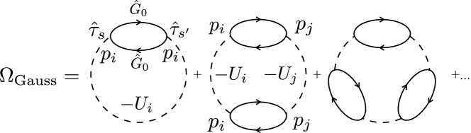
Figure 1: Fluctuation correction $\Omega_{\rm Gauss}$ to the thermodynamic potential $\Omega$ in the $p$-wave Gaussian fluctuation theory. The solid line and the dashed line describe the $2\times 2$-matrix single-particle thermal Green’s function $G_{0}$ in the mean field theory, and the $p$-wave interaction $-p_{i}U_{i}p^{\prime}_{i}$ ($i=x,y,z$), respectively. $\tau_{s=\pm}$ is given by $\tau_{\pm}=\tau_{1}\pm i\tau_{2}$, where $\tau_{j}$ is the Pauli matrix.

We include pairing fluctuations in the $p$-wave Cooper channel within the Gaussian fluctuation theory. In this strong-coupling theory, the thermodynamic potential $\Omega$ consists of the mean field part $\Omega_{\rm MF}$ and the fluctuation part $\Omega_{\rm Gauss}$. $\Omega_{\rm MF}$ is given by

$$\Omega_{\rm MF} = \frac{1}{2}\sum_{i=x,y,z}d^{*}_{i}U^{-1}_{i}d_{i}+\frac{1}{2}\sum_{\bf p}\left[\xi_{p}-E_{p}\right]-\frac{1}{\beta}\sum_{\bf p}\ln\left[1+e^{-\beta E_{p}}\right].$$ (4)

Here, ${\bf d}=(d_{x},d_{y},d_{z})$ is the $p$-wave superfluid order parameter, and $E_{\bf p}=\sqrt{\xi_{p}^{2}+\left|{\bf d}\cdot{\bf p}\right|^{2}}$ describes Bogoliubov single-particle excitations. The fluctuation part, $\Omega_{\rm Gauss}$, is diagrammatically given in Fig.1. Summing up these diagrams, one has

$$\Omega_{\rm Gauss} = \frac{1}{2\beta}\ln\mathrm{det}\left[1+\hat{W}\hat{\pi}({\bf q},i\nu_{n})\right],$$ (5)

where $\hat{W}^{\alpha\beta}_{ij}=U_{i}\delta_{ij}\delta_{\alpha\beta}$ ($\alpha,\beta=1,2$ and $i,j=x,y,z$). $\hat{\pi}^{\alpha\beta}_{ij}$ is the correlation function, having the form,

$$\pi^{11}_{ij}\left({\bf q},i\nu_{n}\right) = \frac{1}{\beta}\sum_{p}p_{i}p_{j}\mathrm{Tr}\left[\tau_{-}G_{0}\left({\bf p+\frac{q}{2}},i\omega_{n}\right)\tau_{+}G_{0}\left({\bf p-\frac{q}{2}},i\omega_{n}-i\nu_{n}\right)\right],$$ (6)

$$\pi^{12}_{ij}\left({\bf q},i\nu_{n}\right) = \frac{1}{\beta}\sum_{p}p_{i}p_{j}\mathrm{Tr}\left[\tau_{-}G_{0}\left({\bf p+\frac{q}{2}},i\omega_{n}\right)\tau_{-}G_{0}\left({\bf p-\frac{q}{2}},i\omega_{n}-i\nu_{n}\right)\right],$$ (7)

$$\pi^{22}_{ij}\left({\bf q},i\nu_{n}\right) = {\pi^{11}_{ij}}^{*}\left({\bf q},i\nu_{n}\right),$$ (8)

$$\pi^{21}_{ij}\left({\bf q},i\nu_{n}\right) = {\pi^{12}_{ij}}^{*}\left({\bf q},i\nu_{n}\right).$$ (9)

Here, $G_{0}({\bf p},i\omega_{n})$ is the $2\times 2$-matrix single-particle thermal Green’s function in the mean field theory, given by

$$G_{0}({\bf p},i\omega_{n})={1\over i\omega_{n}-\xi_{p}\tau_{3}+{\mathrm{Re}}({\bf d\cdot p})\tau_{1}+{\mathrm{Im}}({\bf d\cdot p})\tau_{2}},$$ (10)

where $\tau_{j}$ ($j=1,2,3$) are the Pauli matrices acting on the particle-hole space, and $\tau_{\pm}=\tau_{1}\pm i\tau_{2}$.

As usual, we determine the superfluid order parameter ${\bf d}$ by solving the gap equation

$$d_{i} = \sum_{\bf{p}}U_{i}p_{i}\frac{{\bf d\cdot p}}{2E_{\bf p}}\tanh\frac{\beta E_{\bf p}}{2},$$ (11)

together with the equation for the number $N$ of Fermi atoms,

$$N=-\frac{\partial\Omega}{\partial\mu} = \frac{1}{2}\sum_{\bf p}\left[1-\frac{\xi_{p}}{E_{\bf p}}\tanh\frac{\beta E_{\bf p}}{2}\right]$$ (12)

$$- \frac{1}{2\beta}\sum_{{\bf q},i\nu_{n}}\mathrm{Tr}\left[\left(\hat{W}^{-1}+\hat{\pi}\left({\bf q},i\nu_{n}\right)\right)^{-1}\frac{\partial\hat{\pi}\left({\bf q},i\nu_{n}\right)}{\partial\mu}\right],$$

and determine ${\bf d}$ and the Fermi chemical potential $\mu$ self-consistently.

Since we are taking $U_{x}>U_{y}=U_{z}$, the superfluid phase transition first occurs in the $p_{x}$-wave Cooper channel. Thus, the equation for the superfluid phase transition temperature $T_{\rm c}$ is given by setting $i=x$ and ${\bf d}\to 0$ in Eq. (11), as

$$1=U_{x}\sum_{\bf{p}}\frac{p_{x}^{2}}{2\xi_{p}}\tanh\frac{\beta\xi_{p}}{2}.$$ (13)

We solve this equation, together with the number equation (12) with ${\bf q}=0$, to determine $T_{\rm c}$.

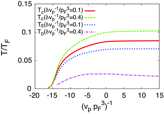
Figure 2: (Color online) Calculated superfluid phase transition temperature $T_{\rm c}$ and the phase transition temperature $T_{0}$ from the $p_{x}$-wave state to the $p_{x}+ip_{y}$-wave state, as functions of the inverse scattering volume $(v_{x}p_{\rm F}^{3})^{-1}$ (where $p_{\rm F}$ is the Fermi momentum). We take $k_{0}=-30.0p_{F}$.

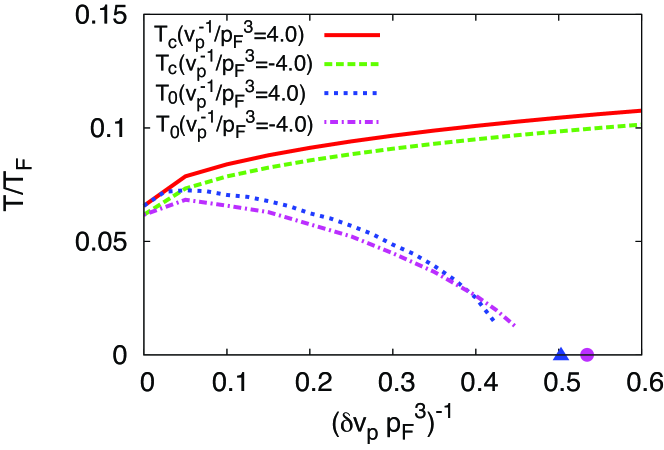
Figure 3: (Color online) Effects of anisotropy ($\delta v_{p}^{-1}=v_{x}^{-1}-v_{y}^{-1}$) on the superfluid transition temperature $T_{\rm c}$ and the phase transition temperature $T_{0}$ from the $p_{x}$-wave state to the $p_{x}+ip_{y}$-wave state. The solid triangle and circle, respectively, show the critical value of $(\delta v_{p}p_{\rm F}^{3})^{-1}$ where $T_{0}$ vanishes with $(v_{x}p_{\rm F}^{3})^{-1}=4.0,-4.0$, calculated within the mean field theory.

3 Superfluid phase transition and transition between $p_{x}$-wave and $p_{x}+ip_{y}$-wave states

Figure 2 shows $T_{\rm c}$ as a function of the interaction strength. In this figure, the increase of the inverse scattering volume $(v_{x}p_{\rm F}^{3})^{-1}$ corresponds to the increase of the interaction strength. Starting from the weak-coupling regime, $T_{\rm c}$ gradually increases with increasing the strength of the pairing interaction, and it approaches a constant value when $(v_{x}p_{\rm F}^{3})^{-1}\ \raise 1.29167pt\hbox{$>$}\kern-8.00003pt\lower 3.01385pt\hbox{$\sim$}\ 0$. Apart from the values of $T_{\rm c}$, the overall behavior of $T_{\rm c}$ is close to the $s$-wave case.

In the weak-coupling regime, Fig. 2 shows that the anisotropy of the pairing interaction (which is described by the anisotropy parameter $\delta v_{p}^{-1}=v_{x}^{-1}-v_{y}^{-1}$) is not crucial for $T_{\rm c}$. In this regard, we note that, since the $T_{\rm c}$ equation (13) does not explicitly involve $U_{y}$ nor $U_{z}$, they only affect $T_{\rm c}$ through the Fermi chemical potential $\mu$ determined by the number equation (12). However, the magnitude of $\mu$ is actually close to the Fermi energy in the weak-coupling regime because of weak pairing fluctuations. Thus, the superfluid phase transition in this regime is only dominated by $U_{x}$ (or $v_{x}$), so that $T_{\rm c}$ is insensitive to $\delta v_{p}^{-1}=v_{x}^{-1}-v_{y}^{-1}$.

The anisotropy of the $p$-wave pairing interaction gradually becomes important, as one goes away from the weak-coupling regime. To understand this, it is convenient to consider the strong coupling limit. In this extreme case, the system may be viewed as a Bose gas, consisting of three kinds of tightly bound molecules that are formed by $U_{x}$, $U_{y}$, and $U_{z}$ pairing interactions. $T_{\rm c}$ is then dominated by the Bose-Einstein condensation of one of the three components having the largest number $N_{\rm B}$ of Bose molecules. While $N_{\rm B}=N/6$ in the isotropic case (where $N$ is the number of the Fermi atoms), $N_{\rm B}$ approaches $N/2$ with increasing the magnitude of $U_{x}$ compared with the other two interactions. Since the BEC phase transition temperature of an ideal Bose gas is proportional to $N_{\rm B}^{2/3}$, $T_{\rm c}$ increases with increasing the anisotropy parameter $\delta v_{p}^{-1}=v_{x}^{-1}-v_{y}^{-1}$.

Although the $p_{x}$-wave superfluid phase is realized near $T_{\rm c}$, this pairing symmetry changes into the $p_{x}+ip_{y}$-wave at a certain temperature ($\equiv T_{0}$) below $T_{\rm c}$, as shown in Fig.2. While $T_{\rm c}$ is larger for a larger value of the anisotropy parameter $\delta v_{p}^{-1}$, $T_{0}$ for $(\delta v_{p}p_{\rm F}^{3})^{-1}=0.4$ is found to be lower than that for $(\delta v_{p}p_{\rm F}^{3})^{-1}=0.1$. To see this more clearly, we show the $(\delta v_{p}p_{\rm F}^{3})^{-1}$-dependence of $T_{0}$ in Fig.3. When the $p$-wave interaction is very anisotropic ($U_{x}\gg U_{y}=U_{z}$), the $p_{x}$-wave pairing becomes more and more favorable, so that the $p_{x}+ip_{y}$-wave state is suppressed. Although it is difficult to examine the region far below $T_{\rm c}$ based on the present strong-coupling theory because of computational problems, we briefly note that a critical value of $\delta v_{p}^{-1}$ at which $T_{0}$ vanishes can be obtained within the mean field theory.

4 Summary

To summarize, we have investigated the superfluid properties of a one-component Fermi gas with an anisotropic $p$-wave interaction. Within the framework of the Gaussian fluctuation theory, we determined the superfluid transition temperature $T_{\rm c}$, as well as the phase transition temperature $T_{0}$ from the $p_{x}$-wave pairing state to the $p_{x}+ip_{y}$-wave state. While the anisotropy of the $p$-wave pairing interaction ($U_{x}>U_{y}=U_{z}$) is not crucial for $T_{\rm c}$ in the weak-coupling regime, we showed that this anisotropy enhances $T_{\rm c}$ in the strong-coupling regime. We also showed that, in contrast to the case of $T_{\rm c}$, the anisotropy of the pairing interaction suppresses $T_{0}$.