One- and two-dimensional reductions of the mean-field description of degenerate Fermi gases

Abstract

We study collective behavior of Fermi gases trapped in various external potentials, including optical lattices (OLs), in the framework of the mean-field (hydrodynamic) description. Using the variational method, we derive effective dynamical equations for the one- and two-dimensional (1D and 2D) settings from the general 3D mean-field equation. The respective confinement is provided by trapping potentials with the cylindrical and planar symmetry, respectively. The resulting equations are nonpolynomial Schrödinger equations (NPSEs) coupled to equations for the local transverse size of the trapped states. Numerical simulations demonstrate close agreement of results produced by the underlying 3D equation and the effective low-dimensional ones. We consider the ground state in these settings. In particular, analytical solutions are obtained for the effectively 2D non-interacting Fermi gas. Differences between the 1D and 2D configurations are highlighted. Finally, we analyze the dependence of the 1D and 2D density patterns of the trapped gas, in the presence of the OL, on the strengths of the confining and OL potentials, and on the scattering length which determines the strength of interactions between non-identical fermions.

1 Introduction

In recent years, ultracold atomic gases have been explored as the means of experimental and theoretical simulations of various aspects of many-body physics [1]-[5]. In particular, conventional solid-state physics can be emulated by gases of fermionic atoms. The possibility to adjust the depth of the optical lattices (OLs), into which the gas is usually loaded, and the strength of interactions between atoms via the Feshbach resonance, opens the way to a detailed experimental study of these settings [6]-[7]. Such possibilities have inspired, in particular, many works dealing with the BCS-BEC crossover [8]-[11], which occurs on the route from weak to strong attraction, being particularly relevant as a simulator of superconductivity.

In these contexts, the density-functional theory (mean field) and the local-density approximation have been used with great success for the description of quantum gases close to their ground states [12]-[18], resulting in effective time-dependent nonlinear Schrödinger equations. In the framework of this approach, hydrodynamic equations for the superfluid Fermi gas at zero temperature were derived in Ref. [19], and, in a similar way, the hydrodynamic equations which remain valid in the presence of temporal variations of control parameters were derived in Ref. [20].

The possibility of highly confined systems in one and two dimensions has stimulated the search for dimensionally reduced descriptions. In particular, quasi-one-dimensional Fermi systems described by many-body Hamiltonians have been analyzed, following seminal works [21, 22] and a more recent one [23]. A variational approach for 1D and 2D Fermi gases in the presence of OL potentials was developed in Ref. [24], and a similar technique for 1D and 2D Fermi-Fermi mixtures was proposed still earlier in works [25] and [26].

In this paper we address Fermi gases in the BCS regime in nearly 2D and 1D configurations, i.e., disk- and cigar-shaped ones, respectively. The configurations may also include inner OL potentials. To reduce the 3D nonpolynomial Schrödinger equation (NPSE) for the Fermi gas, known from the hydrodynamic description, to the corresponding 2D and 1D equations, we use the variational method, similar to that employed in Refs. [27, 28] to reduce the 3D Gross-Pitaevskii equation for the Bose-Einstein condensate to the respective 1D and 2D bosonic NPSEs. Unlike variational methods usually employed in the description of confined fermion systems, which postulate a constant width of the wave-function profile in the confined dimensions, the present method accounts for variations of the confinement width, resulting in significant corrections to the density profile. We demonstrate that our improved approximation is essentially closer to results of the 3D integration.

As a starting point, we derive an effective hydrodynamics equation for a multicomponent Fermi gas with balanced populations, generalizing those found in the literature for a gas with two balanced populations, considering the BCS limit the density of energy. Next, we derive a effective equations for the disk-shaped trap, in the form of the respective equation for the fermionic mean-field wave function coupled to an equation for the transverse width of the trapped state. Analytical solutions of the 2D equations can be found for the non-interacting gas; in the presence of the interactions between fermions with spins up and down, we develop numerical solutions, and demonstrate that the reduced equations reproduce the results obtained from the full 3D equation with a very good accuracy. We further extend the analysis to include the 2D (in-plane) lattice and superlattice potentials. Then, we examine the reduction of the 3D NPSE to 1D equations in the case of the cigar-shaped confinement. The quasi-1D configuration including the axial OL potential is investigated too.

2 The model

2.1 Effective hydrodynamic equation for two balanced populations

We consider a weakly interacting dilute Fermi gas of $N$ atoms of mass $m$ and atomic spin $s$, which form the BCS superfluid, loaded into an optical trap. The gas is taken at zero temperature, with balanced populations of the $2s+1$ possible spin states, as specified in detail below. To do this, we start with the case of balanced populations, for which an effective hydrodynamic equation was derived from the time-dependent density-functional theory for the Fermi gas, in the regime of the BCS-BEC crossover, by Kim and Zubarev in Ref. [19]:

$$i\hbar{\partial_{t}}\Psi\left({\mathbf{r},t}\right)=\left[{\ -\frac{{\hbar^{2}}}{{2m}}{\nabla^{2}}+V\left({\mathbf{r}}\right)+\mu\left(n\left({\mathbf{r},t}\right)\right)}\right]\Psi\left({\mathbf{r},t}\right),$$ (1)

where $\Psi$ is the superfluid wave function, such that $n\left({\mathbf{r},t}\right)={\left|\Psi\left({\mathbf{r},t}\right)\right|^{2}}$ is the particle density, and

$$\mu\left(n\right)=\frac{\partial}{\partial n}\left[{n\varepsilon\left(n\right)}\right]$$ (2)

is the chemical potential, related to the energy per particle $\varepsilon\left(n\right)$. In Ref. [19] it was also shown, for elongated cigar-shaped potential traps, that the von Weizsäcker’s correction to the Thomas-Fermi kinetic-energy density (which corresponds to the hydrodynamic approximation) [29], ${\varepsilon_{\mathrm{TF}}}\left(n\right)=\left({3/10}\right)n{\hbar^{2}}{\left({3{\pi^{2}}n}\right)^{2/3}}/m$, may be important even for the gas with a large density of fermions, $\left|{\nabla n}\right|/{n^{4/3}}\ll 1$ (this is the applicability condition for the hydrodynamic approximation). Such an improved hydrodynamic approximation corresponds to the first two terms of the Kirzhnitz’s gradient expansion [30]. For large smoothly varying densities in the free space, the respective correction is negligible; however, for strongly confined systems the additional term (the kinetic energy) may be comparable to the main one, hence it cannot be neglected, as shown below by our variational approach.

A problem also arises at edges of the trapped superfluid, where $\left|{\nabla n}\right|/{n^{4/3}}$ ceases to be small. To overcome this problem, one may consider the trapped gas with large number of particles, lessening the relative significance of the edges. The case of a relatively small number of particles ($N\sim 10^{2}$) is considered below too, just with the aim to test the accuracy of the variational method.

2.2 The BCS regime

For a fermionic gas composed of two spin states with balanced populations and a negative scattering length of the $s$-wave collisions between the particles in different spin states, ${a_{s}}<0$, the BCS limit corresponds to $k_{F}{\left|{a_{s}}\right|}\ll 1$, with the Fermi wavenumber $k_{F}=(3\pi^{2}n)^{1/3}$. In this regime, the energy per particle, $\varepsilon$, is represented by the expansion in powers of $k_{F}{\left|{a_{s}}\right|}$ [31]:

$$\varepsilon\left(n\right)=\frac{3}{5}{\varepsilon_{F}}\left[{1+\frac{{10}}{{9\pi}}{k_{F}}{a_{s}}+\frac{{4\left({11-2\ln\left(2\right)}\right)}}{{21{\pi^{2}}}}{{\left({{k_{F}}{a_{s}}}\right)}^{2}}+\cdots}\right],$$ (3)

where ${\varepsilon_{F}}={\hbar^{2}}k_{F}^{2}/\left({2m}\right)$ is the Fermi energy. From Eqs. (3) and (2) it follows that the chemical potential takes the form

$$\mu\left(n\right)=\frac{{\hbar^{2}}}{{2m}}{\left({3{\pi^{2}}}\right)^{2/3}}{n^{2/3}}+\frac{{2{\hbar^{2}}\pi{a_{s}}}}{m}n\left[{1+{1.893a_{s}}{n^{1/3}}+\cdots}\right]$$ (4)

where the first term corresponds to the effective Pauli repulsion, and the following ones to the superfluidity due to collisions between the fermions in different spin states. Substituting the latter expression in Eq.(1), and keeping only the first collisional term, we obtain the known nonlinear Schrödinger equation for the fermionic superfluid (see, e.g., Refs. [19, 13]),

$$i\hbar{\partial_{t}}\Psi=\left[{\ -\frac{{\hbar^{2}}}{{2m}}{\nabla^{2}}+V+\frac{{\hbar^{2}}}{{2m}}{{\left({3{\pi^{2}}}\right)}^{2/3}}{n^{2/3}}+\frac{{2\pi{\hbar^{2}}{a_{s}}}}{m}n}\right]\Psi,$$ (5)

where the last term is similar to that in the Gross-Pitaevskii equation for bosons, but with an extra factor of $1/2$, as the Pauli exclusion principle allows only atoms in different spin states interact via the scattering. Equation (5) implies equal particle densities and phases of the wave functions associated with both spin states.

2.3 The effective hydrodynamic equation for multiple balanced populations

We now aim to extrapolate the previous case to systems with multiple atomic spin states, $\sigma_{j}$, associated with $2s+1$ values of the vertical projection of the spin. To this end, we treat the atoms in each spin state ($\sigma_{j}$) as a fully polarized Fermi gas, and include interactions between atoms in the different spin state (assuming a single value of the scattering length, $a_{s}$), which leads to the following system of equations:

$$i\hbar{\partial_{t}}{\Psi_{j}}\left({\mathbf{r},t}\right) = \left[{\ -\frac{{\hbar^{2}}}{{2m}}{\nabla^{2}}+V\left({\mathbf{r}}\right)+\frac{{\hbar^{2}}}{{2m}}{{\left({6{\pi^{2}}}\right)}^{2/3}}{{n_{j}\left({\mathbf{r},t}\right)}^{2/3}}}\right]{\Psi_{j}}\left({\mathbf{r},t}\right)$$ (6)

$$+\frac{{4\pi{\hbar^{2}}{a_{s}}}}{m}\sum\limits_{k\neq j=-(s+1/2)}^{s+1/2}{{{n_{k}\left({\mathbf{r},t}\right)}}{\Psi_{j}}}\left({\mathbf{r},t}\right),$$

where $\Psi_{j}$ is the wave function of the superfluid associated with spin projection $\sigma_{j}$, such that $n_{j}\left({\mathbf{r},t}\right)={\left|{{\Psi_{j}}\left({\mathbf{r},t}\right)}\right|^{2}}$ is the respective particle density, and $V(\mathbf{r})$ an external potential, which is assumed to be identical for all the spin states. A relevant example of a higher nuclear spin, $s=9/2$ (decoupled from the electron states), in a degenerate Fermi gas of ⁸⁷Sr, was demonstrated in Ref. [32].

In the case of fully locally balanced populations, the density of particles is the same in each component, $n_{1}=n_{2}=...=n_{2s+1}$, hence the total density is $n=(2s+1)n_{j}$. Assuming also equal phases of the wave-function components, we define a single wave function, $\Psi=\sqrt{2s+1}\Psi_{j}$, hence Eq. (6) is replaced by

$$i\hbar{\partial_{t}}{\Psi}=\left[-\frac{{{\hbar^{2}}}}{{2{m}}}{\nabla^{2}}+{V}+\frac{{\hbar^{2}}}{{2m}}{{\left({\frac{{6{\pi^{2}}}}{{2s+1}}}\right)}^{2/3}}n_{\mathrm{3D}}^{2/3}+g{n_{\mathrm{3D}}}\right]{\Psi},$$ (7)

with density ${n_{\mathrm{3D}}}\left({{\mathbf{r}},t}\right)={\left|{\Psi\left({{\mathbf{r}},t}\right)}\right|^{2}}$ and scattering coefficient

$$g\equiv 8s\pi{\hbar^{2}}{a_{s}}/(2s+1)m.$$ (8)

In particular, the fully polarized gas, with the interactions between identical fermions suppressed by the Pauli principle, formally corresponds to $s=0$ (hence, $g=0$, as given by Eq. (8)). Unless specified otherwise, we set $s=1/2$ below, focusing on the case of balanced populations in two components.

2.4 The Lagrangian density

Equation (7) can be derived, as the Euler-Lagrange equation,

$$\frac{{\delta\mathcal{L}}}{{\delta{\Psi^{\ast}}}}=\frac{{\partial\mathcal{L}}}{{\partial{\Psi^{\ast}}}}-\frac{\partial}{{\partial t}}\frac{{\partial\mathcal{L}}}{{\partial\left({{\partial_{t}}{\Psi^{\ast}}}\right)}}-\nabla\frac{{\partial\mathcal{L}}}{{\partial\left({\nabla{\Psi^{\ast}}}\right)}}=0,$$ (9)

from the corresponding action, $\mathcal{S}=\int{dtd{\mathbf{r}}\mathcal{L}}$, with the Lagrangian density

$$\mathcal{L} = i\frac{\hbar}{2}\left({{\Psi^{\ast}}\frac{{\partial\Psi}}{{\partial t}}-\Psi\frac{{\partial{\Psi^{\ast}}}}{{\partial t}}}\right)-\frac{{{\hbar^{2}}}}{{2{m}}}{\left|{\nabla{\Psi}}\right|^{2}}-{V}(\mathbf{r}){n_{\mathrm{3D}}}-$$ (10)

$$\frac{{{\hbar^{2}}}}{{2{m}}}\frac{3}{5}{\left({\frac{{6{\pi^{2}}}}{{2{s}+1}}}\right)^{2/3}}n_{\mathrm{3D}}^{5/3}-\frac{1}{2}{g}n_{\mathrm{3D}}^{2},$$

where the asterisk stands for the complex conjugate. Similar Lagrangian formalisms have been used, in the context of the density-functional theory, in diverse settings [13, 26, 33].

Our goal is to reduce the 3D description to one and two dimensions, using the variational approach. As said above, this derivation may be compared to that for the low-dimensional NPSE from the 3D Gross-Pitaevskii equation for the bosonic gas [27, 28]. The approach is based on the factorization of the 3D wave function, substituting the corresponding ansatz into the action, and integrating out the factor corresponding to the direction(s) orthogonal to the confined dimensions.

3 The two-dimensional reduction

3.1 The derivation of the 2D equations

Here we aim to derive effective 2D equations for the Fermi gas in a disk-shaped trap. For this purpose, we consider the external potential composed of two terms: the parabolic (harmonic-oscillator) one accounting for the confinement in the $z$ direction, transverse to the disk’s plane, and the in-plane potential, $V_{\mathrm{2D}}$:

$$V\left({\mathbf{r}}\right)=\frac{1}{2}m\omega_{z}^{2}{z^{2}+}V_{\mathrm{2D}}\left({x,y}\right).$$ (11)

As said above, the initial ansatz assumes the factorization of the 3D wave function into a product of functions of $z$ and $\left(x,y\right)$, the former one being the ground state of the harmonic-oscillator potential [18]:

$$\Psi\left({{\mathbf{r}},t}\right)=\frac{1}{{{\pi^{1/4}}}\sqrt{{\xi{{\left({x,y,t}\right)}}}}}{\exp}\left(-\frac{{{z^{2}}}}{{2}\left({\xi{{\left({x,y,t}\right)}}}\right)^{2}}\right)\phi\left({x,y,t}\right),$$ (12)

subject to the unitary normalization, with transverse width $\xi(z,t)$ considered as a variational function, while the 2D wave function, $\phi$, is normalized to the number of atoms. Therefore, the reduction from 3D to 2D implies that the system of equations should be derived for the pair of functions $\phi\left(x,y,t\right)$ and $\xi\left(x,y,t\right)$, using the reduced action functional to be derived by integrating the 3D action over the $z$-coordinate (cf. the derivation for the bosonic gas [27, 28]):

$$\mathcal{S}{{}_{\mathrm{2D}}}=\int{dtdxdy{\mathcal{L}}_{\mathrm{2D}}},$$ (13)

where the respective Lagrangian density is

$${\mathcal{L}_{\mathrm{2D}}} = i\frac{\hbar}{2}\left({{\phi^{\ast}}{\partial_{t}}\phi-\phi{\partial_{t}}{\phi^{\ast}}}\right)-\frac{{\hbar^{2}}}{{2m}}{\left|{{\nabla_{\bot}}\phi}\right|^{2}}-{V_{\mathrm{2D}}n_{\mathrm{2D}}}$$ (14)

$$-\left[\frac{{\hbar^{2}}}{{2m}}\frac{{3C_{\mathrm{2D}}}}{{5{\xi^{2/3}}}}n_{{\mathrm{2D}}}^{5/3}+\frac{g}{{2{{\left({2\pi}\right)}^{1/2}}\xi}}n_{{\mathrm{2D}}}^{2}+\frac{{\hbar^{2}}}{{4m{\xi^{2}}}}{n_{{\mathrm{2D}}}}+\frac{{m\omega_{z}^{2}{\xi^{2}}}}{4}{n_{{\mathrm{2D}}}}\right],$$

with 2D density ${n_{\mathrm{2D}}}\left(x,y\right)={\left|\phi\left(x,y\right)\right|^{2}}$, $C_{\mathrm{2D}}\equiv{(3/5)^{1/2}(6/(2s+1))^{2/3}}\pi$. The last two terms in Eq. (14) result from the reduction to 2D: the first among them shows that stronger confinement implies a higher energetic cost, while the quadratic dependence on $\xi$ in the last term originates from the original confining potential acting in the $z$ direction. These two terms are relevant for configurations with an inhomogeneous spatial density, while for spatially homogeneous solutions they may be omitted.

Atoms	$\mathop{\omega_{c}\mathrm{[Hz]}}\limits_{a_{c}=0.1\times{10^{-6}}\mathrm{m}}$	$\mathop{\omega_{c}\mathrm{[Hz]}}\limits_{a_{c}=1.0\times{10^{-6}}\mathrm{m}}$	$\mathop{\omega_{c}\mathrm{[Hz]}}\limits_{a_{c}=10.0\times{10^{-6}}\mathrm{m}}$
6Li	$10.5\times 10^{5}$	$10.5\times 10^{3}$	$105.$
40K	$1.58\times 10^{5}$	$1.58\times 10^{3}$	$15.8$
84Sr	$0.75\times 10^{5}$	$0.75\times 10^{3}$	$7.5$

Table 1: Relevant values of the characteristic frequency, $\omega_{c}$, for ⁶Li, ⁴⁰K and ⁸⁴Sr, assuming three possible values of the characteristic length, $a_{c}$.

To present the effective 2D equations in a dimensionless form, we define a characteristic length, $a_{c}$, and a characteristic frequency, $\omega_{c}$, related through the atomic mass ($m$), $\omega_{c}=\hbar/(ma_{c}^{2})$. In this way, the physical units of the system depend on fix the value of $a_{c}$ (or $\omega_{c}$) for particular atomic species, see Table 1. Thus, we rescale the variables and constants as $\tau\equiv\omega_{c}t/2$, $\left\{X,Y\right\}\equiv\left\{x,y\right\}/a_{c}$, $\vartheta\equiv{a_{c}}\phi$, ${\rho_{\mathrm{2D}}}\equiv{\left|\vartheta\right|^{2}}$, $\zeta\equiv\xi/{a_{c}}$, $U_{\mathrm{2D}}\equiv 2V_{\mathrm{2D}}/(\hbar\omega_{c})$, $G_{\mathrm{2D}}\equiv{2^{7/2}}\sqrt{\pi}s{a_{s}}/\left[{(2s+1)a_{c}}\right]$, and $\varpi_{z}\equiv\omega_{z}/\omega_{c}$. In this notation, time $t$ is expressed in units of $2/\omega_{c}$, and 2D coordinates $\left\{{x,y}\right\}$ in units of $a_{c}$. Then, Eqs. (13) and (14) are transformed into

$$\mathcal{S}=\hbar\int{d\tau dXdY{\tilde{\mathcal{L}}}_{\mathrm{2D}}}$$ (15)

and

$${{{\tilde{\mathcal{L}}}}_{\mathrm{2D}}} = \frac{i}{2}\left({\vartheta^{\ast}{\partial_{\tau}}\vartheta-\vartheta{\partial_{\tau}}\vartheta^{\ast}}\right)-{\left|{\nabla\vartheta}\right|^{2}}-{U_{\mathrm{2D}}\rho_{\mathrm{2D}}}$$ (16)

$$-\left[\frac{3}{{5{\zeta^{2/3}}}}C_{\mathrm{2D}}\rho_{\mathrm{2D}}^{5/3}+\frac{G_{\mathrm{2D}}}{{2\zeta}}\rho_{2D}^{2}+\frac{1}{{2{\zeta^{2}}}}{\rho_{\mathrm{2D}}}+\frac{1}{2}\varpi_{z}^{2}{\zeta^{2}}{\rho_{\mathrm{2D}}}\right],$$

where the part in the square brackets corresponds to the local energy density, $\varepsilon_{\mathrm{2D}}$, when the system is in a spatially homogeneous state in the absence of external potentials:

$${{\varepsilon}_{\mathrm{2D}}}=\frac{3}{{5{\zeta^{2/3}}}}C_{\mathrm{2D}}\rho_{\mathrm{2D}}^{5/3}+\frac{G_{\mathrm{2D}}}{{2\zeta}}\rho_{\mathrm{2D}}^{2}+\frac{1}{{2{\zeta^{2}}}}{\rho_{\mathrm{2D}}}+\frac{1}{2}\varpi_{z}^{2}{\zeta^{2}}{\rho_{\mathrm{2D}}}~{}.$$ (17)

The latter equation is a relation between the energy and particle densities, demonstrating how different interaction terms affect the local stability of the matter wave.

The Euler-Lagrange equations produced by varying action $\mathcal{S}$ with respect to $\vartheta$ and $\zeta$ take the form of

$$i{\partial_{\tau}}\vartheta=\left[-\nabla_{\bot}^{2}+{U_{\mathrm{2D}}}+{\frac{1}{{{\zeta^{2/3}}}}C_{\mathrm{2D}}{{\left|\vartheta\right|}^{4/3}}+\frac{G_{\mathrm{2D}}}{\zeta}{{\left|\vartheta\right|}^{2}}+\frac{1}{{2{\zeta^{2}}}}+\frac{{\varpi_{z}^{2}}}{2}{\zeta^{2}}}\right]\vartheta,$$ (18)

$$\varpi_{z}^{2}{\zeta^{4}}-\frac{2}{5}{C_{\mathrm{2D}}\left|\vartheta\right|^{4/3}}{\zeta^{4/3}}-\frac{1}{2}{G_{\mathrm{2D}}\left|\vartheta\right|^{2}}\zeta-1=0,$$ (19)

cf. Eq. (9). Algebraic equation (19) for $\zeta$ cannot be solved analytically, therefore we used the Newton method to solve it numerically. The necessity to find $\zeta$ at each step of the integration is a numerical complication of a minimal cost compared to the 3D integration of the underlying equation (7).

Nevertheless, for the non-interacting gas, with $G_{\mathrm{2D}}=0$, Eq. (19) is a cubic equation for $\zeta^{4/3}$, which admits an analytical solution, the single physically relevant real root being

$${\varpi_{z}^{2/3}}{\zeta^{4/3}}\left(\Omega\right)=\frac{{2}^{1/3}{\Omega}}{{3}\left({\sqrt{1-\frac{4}{{27}}{\Omega^{3}}}+1}\right)^{1/3}}+\frac{\left({\sqrt{1-\frac{4}{{27}}{\Omega^{3}}}+1}\right)^{1/3}}{{2}^{1/3}},$$ (20)

where $\Omega\equiv 2C_{\mathrm{2D}}\left|\vartheta\right|^{4/3}/(5\varpi_{z}^{2/3})$. This root is real at ${\rho_{\mathrm{2D}}}/{\varpi_{z}}<{5^{9/4}}(2s+1)/({2^{7/2}}{3^{1/4}}{\pi^{3/2}})\approx 0.45(2s+1)$, i.e., for sufficiently low densities and the strong transverse confinement. Further, in the low-density limit, the approximation for the root is

$$\zeta\approx\frac{1}{{{\varpi_{z}^{1/2}}}}\left({1+\frac{C_{\mathrm{2D}}}{{10\varpi_{z}^{2/3}}}{{\left|\vartheta\right|}^{4/3}}}\right),$$ (21)

the substitution of which into Eq. (18) results in the following NPSE for $\vartheta$:

$$i{\partial_{\tau}}\vartheta=\left[{-\nabla_{\bot}^{2}+{U}_{\mathrm{2D}}+\varpi_{z}^{1/3}C_{\mathrm{2D}}\left({{{\left|\vartheta\right|}^{4/3}}-\frac{{C_{\mathrm{2D}}{{\left|\vartheta\right|}^{8/3}}}}{{15\varpi_{z}^{2/3}}}}\right)}\right]\vartheta,$$ (22)

where the chemical potential is shifted by a constant term, $2\varpi_{z}$. In the limit of ${\left|\vartheta\right|\rightarrow 0}$, Eq. (21) yields $\zeta={{\varpi_{z}^{-1/2}}}$, which corresponds to the width of the ground state of the harmonic oscillator.

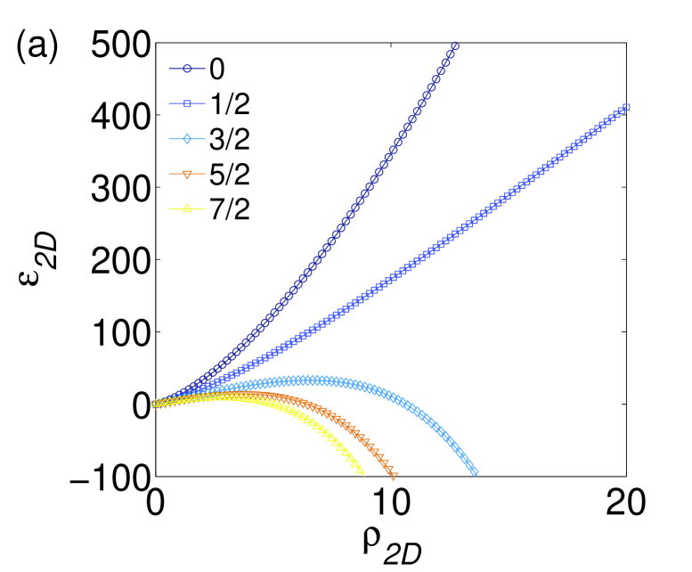
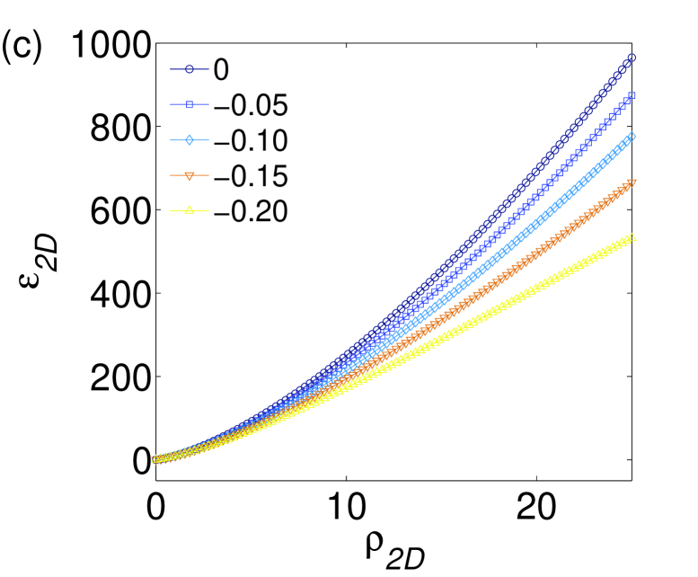
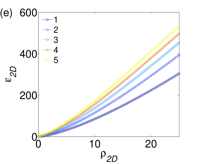
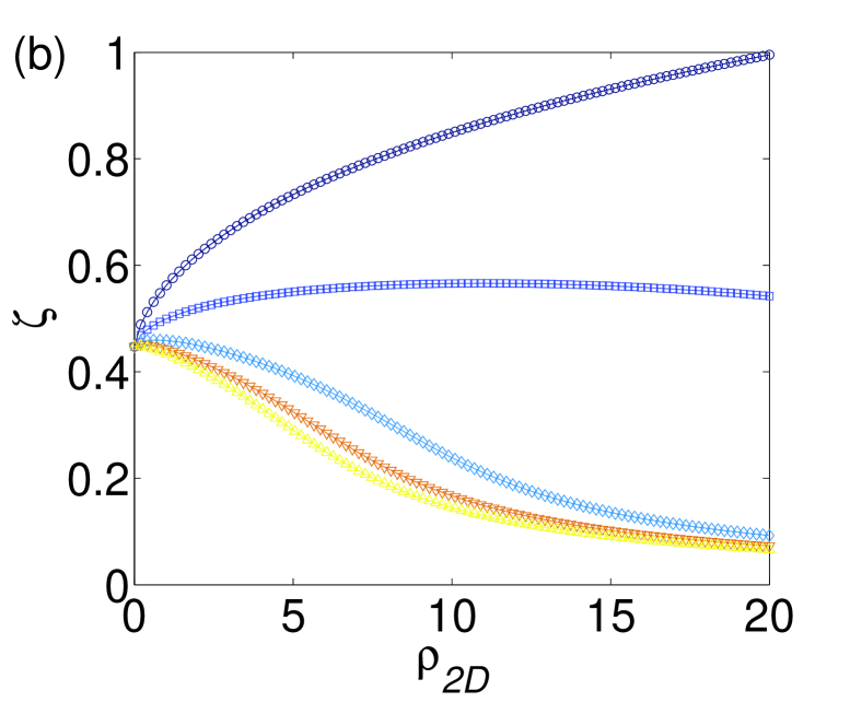
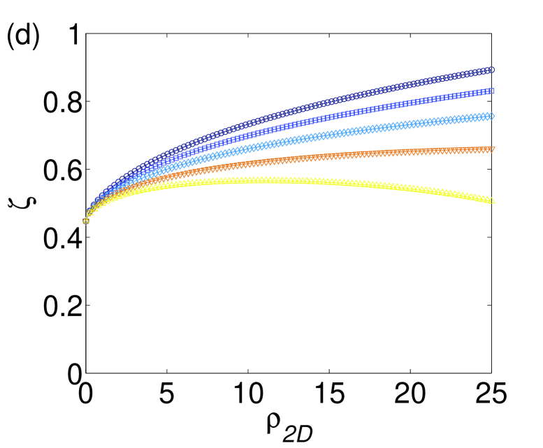
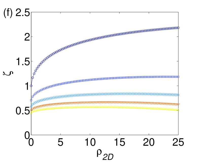
Figure 1: (Color online) The energy density and transverse size, ${{\varepsilon}_{\mathrm{2D}}}$ and $\zeta$, versus the 2D atomic density, $\rho_{\mathrm{2D}}$. (a)  and (b): The dependences are shown for five different values of the spin, $s=0,1/2,3/2,5/2$ and $7/2$, at the fixed negative scattering length, ${a_{s}}/a_{c}=-0.2$, and fixed confinement strength, ${\varpi}_{z}=5$. (c) and (d): The same for five different values of the scattering length, $a_{s}/a_{c}=0,-0.05,-0.10,-0.15$ and $-0.20$, while $s=1/2$ and ${\varpi}_{z}=5$ are fixed. (e) and (f): For five different values of the transverse-confinement strength, ${{\varpi}_{z}}=1,2,3,4$ and $5$, at fixed $s=1/2$ and ${a_{s}}/a_{c}=-0.2$. The optical lattice is absent in all the cases.

The plots in Fig. 1 display the dependence of the energy density $\varepsilon_{\mathrm{2D}}$ and transverse width $\zeta$ on the 2D density $\rho_{\mathrm{2D}}$ for the states uniform in the $\left(x,y\right)$ plane, as produced by Eqs. (17) and Eq. (19), respectively (recall that ${\rho_{\mathrm{2D}}}\equiv{\left|\vartheta\right|^{2}}$). In particular, Figs. 1(a) and  1(b) show how these dependences are affected by the fermion’s spin, $s$. In Fig. 1(a), the energy density of the polarized gas, with $s=0$, is a growing function of the atomic density, since in this case Eq. (8) gives $g=0$, i.e., the Pauli exclusion principle suppresses the interaction between the fermions, as mentioned above. When the gas is composed of equal numbers of atoms with spins up and down ($s=1/2$), the attraction ($a_{s}<0$) between atoms with opposite directions of the spin causes a decrease in the energy density, in comparison to the fully polarized gas. For the cases of $s=3/2,5/2$ and $7/2$, it is observed that a maximum of the energy density is attained at some atomic density ($\rho_{\mathrm{2D},\max}$), due to the greater contribution of the attractive interactions in comparison with the quantum pressure. In agreement with this trend, $\rho_{\mathrm{2D},\max}$ is seen to be smaller for higher values of $s$, as the greater number of possible spin states allows each atom to directly interact with a larger number of atoms in other spin states. Furthermore, Fig. 1(b) shows that (for the same parameters as in Fig. 1(a)) the gas with $s=1/2$ slowly shrinks in the transverse direction ($\zeta$ gradually decreases) with the increase of the 2D density, after attaining a weakly pronounced maximum at certain value of $\rho_{\mathrm{2D}}$. It is also observed that, at the vanishingly small density, the transverse size does not depend of spin $s$, in agreement with Eq. (21). On the other hand, Figs. 1(c) and  1(d) show that, for $s=1/2$, the energy density remains a growing function of the atomic density for all the values of $a_{s}/a_{c}$ considered, and, naturally, the growth is steeper for smaller absolute values of the negative scattering length. Further, the curves in Fig. 1(e) show that the energy density grows steeper when the confinement strength, $\varpi_{z}$, is higher, and, naturally, the tighter confinement leads to the smaller transverse size, as seen in Fig. 1(f). In summary, for $s>1/2$ and in the range of the particle density ($\rho_{\mathrm{2D}}$) considered here (see Fig. 1(a)), the energy density ($\varepsilon_{\mathrm{2D}}$) is an increasing function of the particle density up to a certain value of the density ($\rho=\rho_{\mathrm{2D,}\max}$), where $\varepsilon_{\mathrm{2D}}$ attains a maximum, which it followed by the decrease of the energy density. It is also observed that attaining this maximum is always preceded by the gradual tightening of the gas in the confined direction and increase of the particle density. In dynamical simulations, the system suffers the collapse if the initial particle density exceeds the maximum value $\rho_{\mathrm{2D,}\max}$ (in a nonuniform configurations, the particles are pulled towards the point where this maximum is reached), i.e., $\rho_{\mathrm{2D,}\max}$ is a separatrix bordering between stable and unstable uniform states, cf. similar results reported in Refs. [26, 34, 35].

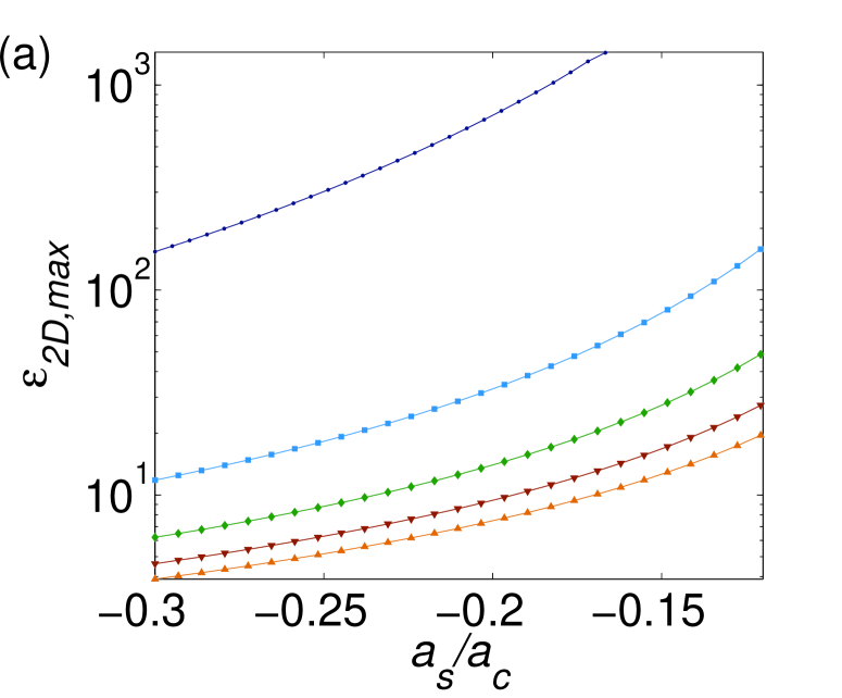
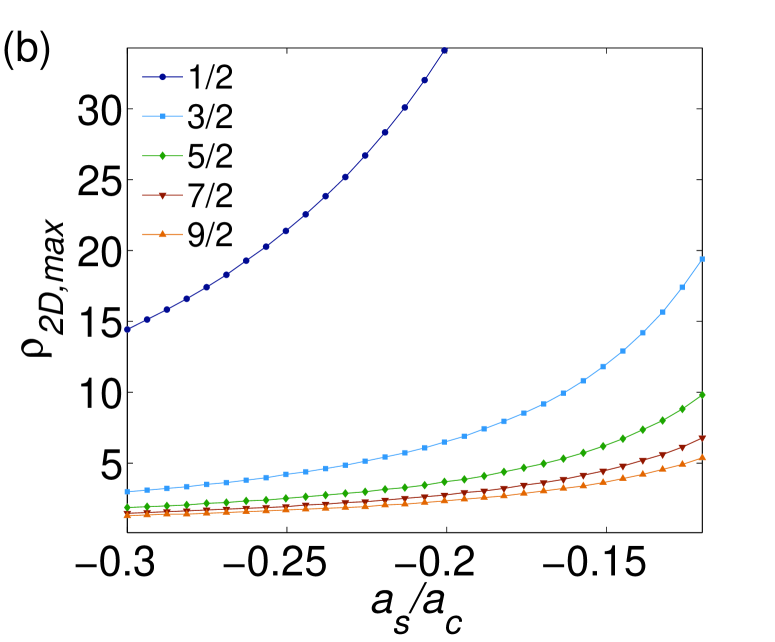
Figure 2: (Color online) (a) The maximum of the 2D energy density, $\varepsilon_{\mathrm{2D},\max}$, as a function of the negative scattering length, $a_{s}/a_{c}$. (b) The 2D atomic density, $\rho_{\mathrm{2D},\max}$, at which $\varepsilon_{\mathrm{2D}}$ attains its maximum. The curves in both plots correspond to five different values of spin $s$, as indicated in the inset in (b). The confinement strength is fixed to be $\varpi_{z}=5$, and the optical lattice is absent here.

Figure 2 shows the maximum value of the energy density as a function of the strength of the attraction between the fermions in the different spin states. It is seen that the enhancement of the attraction causes a transition to lower energy and atomic densities. This behavior is stronger pronounced for lower values of the spin, as a result of the larger relative strength of the Pauli repulsion, leading to greater variations in the energy-density maximum. It should be stressed, though, that these results are approximate due to limitations imposed by the BCS regime (overall, the weak interaction). Actually, most calculations reported in this work were performed for the energy densities far from the maximum value.

After the consideration of the spatially uniform states, the main objective of our analysis is to identify the ground state of the fermion gas loaded into the 2D potential consisting of the harmonic-oscillator trap and square OL,

$${U_{{\mathrm{2D}}}}=\varpi_{x}^{2}{X^{2}}+\varpi_{y}^{2}{Y^{2}}+{A_{x}}{\sin^{2}}\left({{\kappa_{x}}X}\right)+{A_{y}}{\sin^{2}}\left({{\kappa_{y}}Y}\right),$$ (23)

where $\kappa_{x,y}\equiv 2\pi/\lambda_{x,y}$ are the lattice wavenumbers. We start the presentation of the results for nearly-2D trapped Fermi gas in the absence of the OL.

3.2 The trapped quasi-2D gas in the absence of the optical lattice

First, we have verified the accuracy of the 2D reduction by comparing results generated by this approximation versus those obtained by integrating the 3D equation (7). The ground state was found by means of the imaginary-time integration based on the fourth-order Runge-Kutta algorithm. The comparison is produced in Fig. 3, where the radial-density profiles are plotted for the isotropic 2D harmonic-oscillator trap ($\varpi_{x}=\varpi_{y}$), showing an excellent agreement between the 2D and full 3D descriptions. Actually, this is one of main results of the present work.

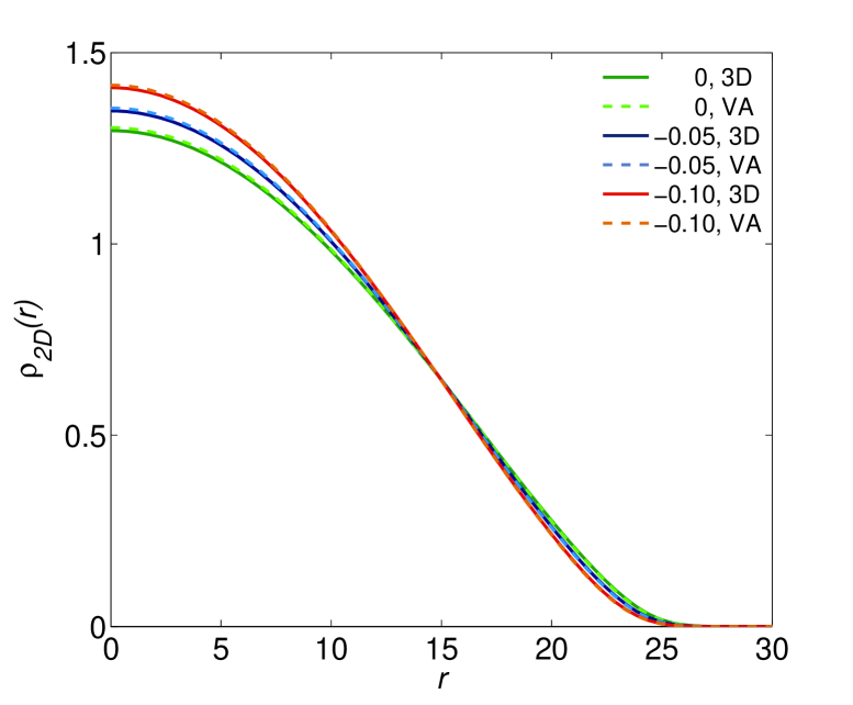
Figure 3: (Color online) The 2D radial density, $\rho_{\mathrm{2D}}(r)$, as obtained from the full 3D equation, and from the 2D reduction based on the variational approximation (“VA”) for the weak isotropic harmonic-oscillator trap acting in the 2D plane ($\varpi_{x}=\varpi_{y}=0.1$, $\varpi_{z}=2$), and $N=1000$. Different curves correspond to the indicated values of $a_{s}/a_{c}=0,-0.05$ and $-0.1$. The optical-lattice potential is absent in this case.

3.3 Effects of the optical lattice

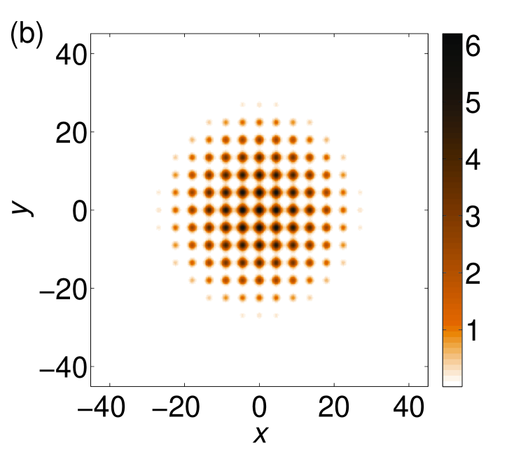
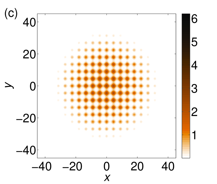
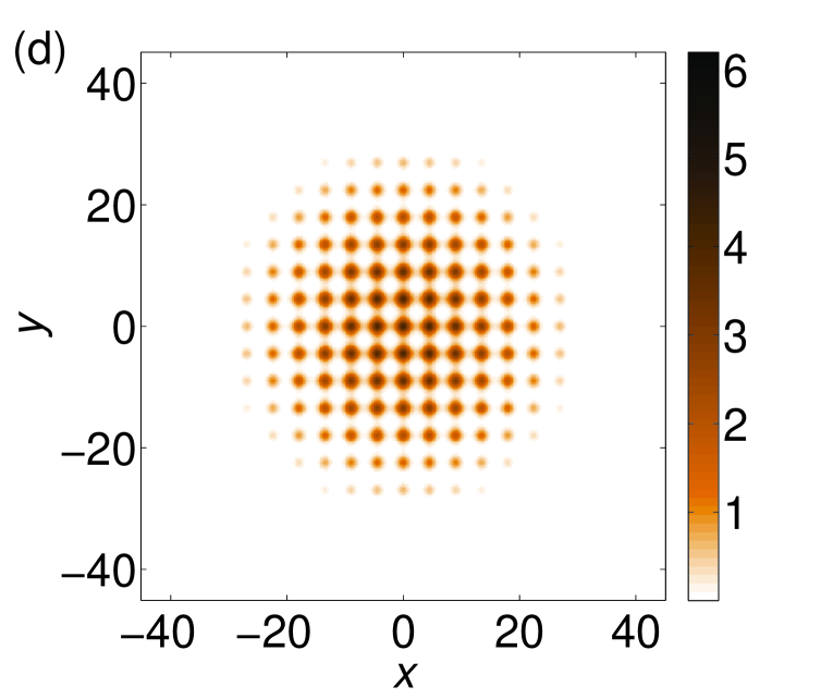
Figure 4: (Color online) Results for the quasi-2D gas trapped in the combination of the optical lattice and weak harmonic-oscillator potential. The plots display density profiles, $\rho_{\mathrm{2D}}(x,y)$, for four cases: (a) $a_{s}/a_{c}=0$ and $\varpi_{z}=2$, (b) $a_{s}/a_{c}=-0.2$ and $\varpi_{z}=2$, (c) $a_{s}/a_{c}=0$ and $\varpi_{z}=8$, and (d) $a_{s}/a_{c}=-0.2$ and $\varpi_{z}=8$. The remaining parameters are $N=1000$, $\varpi_{x}=\varpi_{y}=0.1$, $A_{x}=A_{y}=10$, and $\lambda_{x}=\lambda_{y}=9$.

The plots in Fig. 4 show the density distribution in the ground state of the gas loaded into the 2D harmonic-oscillator potential combined with the 2D square OL (see Eq. 23). Naturally, density peaks coincide with local minima of the OL potential. Figures 4(a) and 4(b) demonstrate that the attractive interaction leads to a decrease in the number of peaks visible in the density profile, and to an increase in their heights. On the other hand, Figs. 4(c) and  4(d) show that, for the same interaction strength as above, tighter transverse confinement results in a greater number of peaks, with a lower atomic density at them. Due to the symmetry of the OL, the number of visible peaks must be in multiples of $4$. We define as “observable” an area with density $\rho_{\mathrm{2D}}\geq 0.1$. The plot of Fig. 5(a) shows the dependence of the observable number of peaks on the transverse-confinement strength $\varpi_{z}$, for $a_{s}/a_{z}=0$ (green circles) and $a_{s}/a_{z}=-0.2$ (blue squares). At all values of $\varpi_{z}$, the number of visible peaks is higher in the $a_{s}=0$ case, with a clear nonlinear dependence that is characterized by intervals in the scale of in $\varpi_{z}$ corresponding to particular numbers of the peaks. This feature is particularly noticeable in the range of $\varpi_{z}=[5,10]$.

Figures 5(b) and  5(c) show detail of the peaks characterization, which amounted to counting the number of peaks in seven specific zones of values of $\rho_{\mathrm{2D}}$: [0.1,1[, [1,2[, [2,3[, [3,4[, [4,5[, [5,6[ and [6,7[. The findings uncover intricate changes in the density patterns, following variations of the system’s parameters. In particular, Fig. 5(b) shows that, for $a_{s}/a_{z}=-0.2$, distinct zones of the values of $\varpi_{z}$ may cluster at the same number of peaks, suggesting that a given number of peaks may be realized in various configurations. The plot in Fig. 5(c) shows the non-interacting case, $a_{s}=0$, with no visible peak in the last two ranges, which implies greater expansion of the gas in the 2D plane. In each range, the variation of parameters significantly alters the distribution of peaks. The multitude of the different coexisting robust multi-peak patterns suggests that this setting has a potential for the use as a data-storage system.

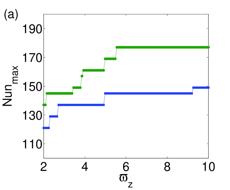
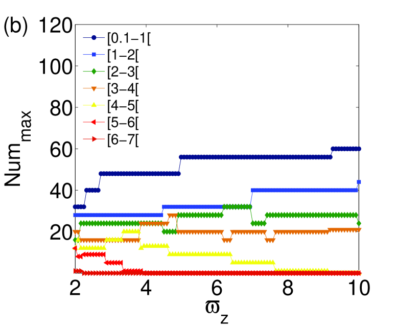
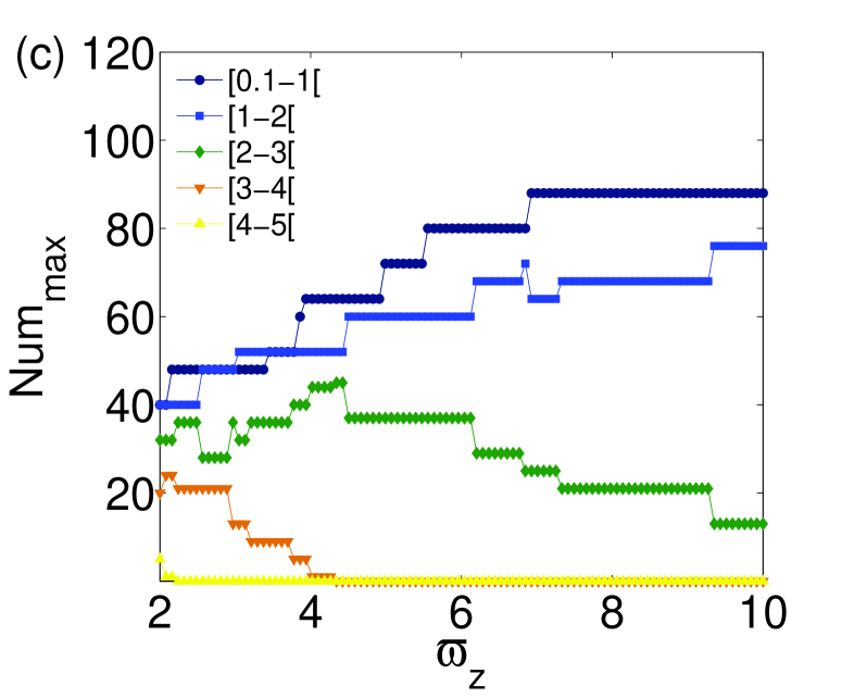
Figure 5: (Color online) (a) The number of density peaks, located at minima of the OL potential, as a function of confinement strength $\varpi_{z}$. The area occupied by the gas is defined as that with $\rho_{\mathrm{2D}}\geq 0.1$. The blue and green lines correspond to $a_{s}/a_{c}=-0.2$ and $a_{s}/a_{z}=0$, respectively. Panels (b) and (c) display, severally, detailed pictures for $a_{s}/a_{c}=-0.2$ and $a_{s}/a_{c}=0$, in seven different ranges of density$\rho_{\mathrm{2D}}$, as indicated in the inset. The parameters are $N=1000$, $\varpi_{x}=\varpi_{y}=0.1$, $A_{x}=A_{y}=10$, and $\lambda_{x}=\lambda_{y}=9$.

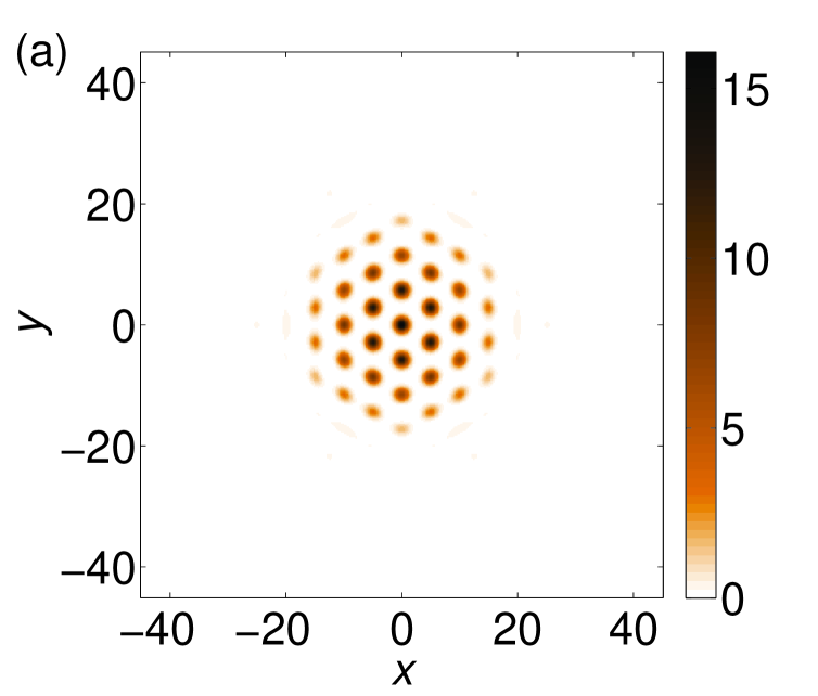
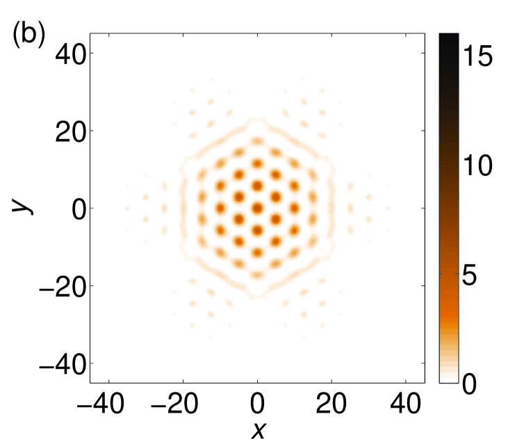
Figure 6: (Color online) The same as in Fig. 4 for the superlattice built of two triangular OLs with angle $\theta=8^{\circ}$ between them: (a) $a_{s}/a_{z}=-0.2$, $\varpi_{z}=2$; (b) $a_{s}/a_{z}=0$, $\varpi_{z}=5$. The other parameters are $N=1000$, $\varpi_{x}=\varpi_{y}=0.1$, and $A_{T}=5$, $\lambda_{T}=10$.

Figure 6 displays the results for the Fermi gas in the presence of a superlattice formed by a superposition of two triangular lattice, each formed by the set of three pairs of counter-propagating laser-beams, with angles $60^{\circ}$ between them, and equal amplitudes and wavelengths. To build the superlattice, we fix the first pair of beams in the $x$-direction in both triangular lattices, and then rotate the two lattices clockwise and counterclockwise by $\pm 4^{\circ}$. The overall shape of the thus formed superlattice remains hexagonal. It is observed that the density maxima are most visible within the central hexagon. The set of different patterns trapped in the superlattice is richer than in the case of the square OL considered above, as different potential minima of the superlattice potential have different depths.

4 The one-dimensional reduction

4.1 The derivation of the 1D equations

To perform the reduction of the mean-field description from 3D to 1D, we consider an external potential formed by the harmonic-oscillator potential in the $\left(x,y\right)$-plane, which represents the cylindrically symmetric magnetic confinement, and an axial ($z$-dependent) potential:

$$V\left({{\mathbf{r}},t}\right)=\frac{1}{2}m\omega_{\mathrm{t}}^{2}r^{2}+V_{\mathrm{1D}}\left({z,t}\right),$$ (24)

where $r\equiv\sqrt{x^{2}+y^{2}}$. Again, the initial ansatz assumes the factorization of the 3D wave function into a product of $r$- and $z$-dependent functions. The former one is taken as the ground state of the 2D harmonic oscillator, hence the ansatz is

$$\Psi\left({{\mathbf{r}},t}\right)=\frac{1}{\sqrt{{\pi}}{\sigma\left({z,t}\right)}}{\exp}\left(-\frac{r^{2}}{{2\sigma}^{2}{{{\left({z,t}\right)}}}}\right)f\left({z,t}\right),$$ (25)

where the 1D wave function, $f\left(z,t\right)$, is normalized to the number of atoms, $N$, and the axial density is defined as $n_{\mathrm{1D}}\equiv\left|f\right|^{2}$. Variational functions $f$ and $\sigma$ can be determined by the minimization of the 3D action after performing the integration in the $\left(x,y\right)$ plane, cf. the derivation of the 1D NPSE for the bosonic gas [27]. This procedure gives rise to the effective 1D Lagrangian density,

$${\mathcal{L}_{\mathrm{1D}}} = i\frac{\hbar}{2}\left({{{f^{\ast}}}{\partial_{t}}{f}-{f}{\partial_{t}}{{f^{\ast}}}}\right)-\frac{{{\hbar^{2}}}}{{2{m}}}{\left|{{\partial_{z}}{f}}\right|^{2}}-{V_{\mathrm{1D}}n_{\mathrm{1D}}}$$ (26)

$$-\left[\frac{{{\hbar^{2}}}}{{2{m}}}\frac{3}{{5\sigma^{4/3}}}C_{\mathrm{1D}}n_{\mathrm{1D}}^{5/3}+\frac{{g}}{{4\pi\sigma^{2}}}n_{\mathrm{1D}}^{2}+\frac{{\hbar^{2}}}{{2m{\sigma^{2}}}}{n_{{\mathrm{1D}}}}+\frac{1}{2}m\omega_{t}^{2}{\sigma^{2}}{n_{{\mathrm{1D}}}}\right],$$

where $C_{\mathrm{1D}}\equiv(3/5)(6\pi/(2s+1))^{2/3}$, $s$ is the fermionic spin, as before, and the last two terms are the result of integration, which keeps the 3D characteristics of the underlying system: When the gas is homogeneous and the external potential is absent, the latter term is irrelevant.

Similar to the 2D case, the normalization is performed with characteristic length scale $a_{c}$ and frequency $\omega_{c}$, so that $Z\equiv z/a_{c}$, $\psi\equiv a_{c}^{1/2}f$, $U_{\mathrm{1D}}\equiv 2V_{\mathrm{1D}}/(\hbar\omega_{c})$, $G_{\mathrm{1D}}\equiv 8sa_{s}/(2s+1)a_{c}$, $\eta\equiv\sigma/a_{c}$, and $\varpi_{\mathrm{t}}\equiv\omega_{\mathrm{t}}/\omega_{c}$. In addition, we define the dimensionless 1D atom density, $\rho_{\mathrm{1D}}\equiv\left|{\psi}\right|^{2}$. Then, the normalized Lagrangian density is

$${{\tilde{\mathcal{L}}}_{\mathrm{1D}}} = \frac{i}{2}({{\psi^{\ast}}}{\partial_{\tau}}{\psi}-{\psi}{\partial_{\tau}}{{\psi^{\ast}}})-{\left|{{\partial_{Z}}{\psi}}\right|^{2}}-{U_{\mathrm{1D}}{\rho}_{\mathrm{1D}}}$$ (27)

$$-\left[\frac{3}{{5{\eta^{4/3}}}}{C_{{\mathrm{1D}}}}\rho_{1D}^{5/3}+\frac{1}{{2{\eta^{2}}}}{G_{{\mathrm{1D}}}}\rho_{1D}^{2}+\varpi_{t}^{2}{\eta^{2}}{\rho_{{\mathrm{1D}}}}+\frac{1}{{\eta^{2}}}{\rho_{{\mathrm{1D}}}}\right].$$

The 1D energy density $\varepsilon_{\mathrm{1D}}$ for uniform states is

$$\varepsilon_{\mathrm{1D}}=\frac{3}{{5{\eta^{4/3}}}}{C_{{\mathrm{1D}}}}\rho_{1D}^{5/3}+\frac{1}{{2{\eta^{2}}}}{G_{{\mathrm{1D}}}}\rho_{1D}^{2}+\varpi_{\mathrm{t}}^{2}{\eta^{2}}{\rho_{{\mathrm{1D}}}}+\frac{1}{{\eta^{2}}}{\rho_{{\mathrm{1D}}}},$$ (28)

cf. Eq. (17) in the 2D case, which makes it possible to compare contributions of the different interactions involved. In fact, the comparison is not straightforward, because of the dependence of $\eta$ on $\rho_{\mathrm{1D}}$; however, for very low densities $\eta$ may be assumed constant, in which case the last two terms dominate in $\varepsilon_{\mathrm{1D}}$. Now, varying the action with respect to $\psi$, we derive the respective Euler-Lagrange equation (similar to the Eq. 9):

$$i{\partial_{\tau}}{\psi}=\left[{-\partial_{Z}^{2}+{U}_{\mathrm{1D}}}+\frac{{C_{\mathrm{1D}}}}{{\eta^{4/3}}}{\left|{\psi}\right|^{4/3}}+\frac{{G_{\mathrm{1D}}}}{{\eta^{2}}}{\left|{\psi}\right|^{2}}+\frac{1}{{\eta^{2}}}+{\varpi_{\mathrm{t}}^{2}}\eta^{2}\right]{\psi},$$ (29)

which is the 1D equation of motion, with powers of the transverse width, $\eta$, in the collisional and Pauli terms being different from their counterparts in the 2D equation, cf. Eq. (18). Further, varying the action with respect to $\eta$ gives rise to the corresponding Euler-Lagrange equation,

$$\varpi_{t}^{2}{\eta^{4}}-\frac{2}{5}C_{\mathrm{1D}}{\left|\psi\right|^{4/3}}{\eta^{2/3}}-\left({1+\frac{G_{\mathrm{1D}}}{2}{{\left|\psi\right|}^{2}}}\right)=0,$$ (30)

which establishes the dependence of the transverse size, $\eta$, on density $\rho_{\mathrm{1D}}$. Generally, this equation should be solved numerically. In the low-density limit, it has a trivial solution, $\eta^{2}=1/\varpi_{\mathrm{t}}$, which, if substituted in Eq. (29) allows one to derive a closed-form equation for $\psi$ [similar to the situation for the same limit in the 2D case, cf. Eq. (22)]:

$$i{\partial_{\tau}}\psi=\left[{-\partial_{Z}^{2}+{U}_{\mathrm{1D}}+C_{\mathrm{1D}}\varpi_{\mathrm{t}}^{2/3}{{\left|\psi\right|}^{4/3}}+{\varpi_{\mathrm{t}}}G_{\mathrm{1D}}{{\left|\psi\right|}^{2}}+2{\varpi}}_{t}\right]\psi,$$ (31)

with the lowest-order nonlinear term accounting for the Pauli repulsion of the same type as in the 2D equation (22).

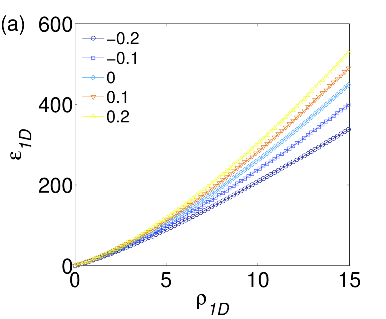
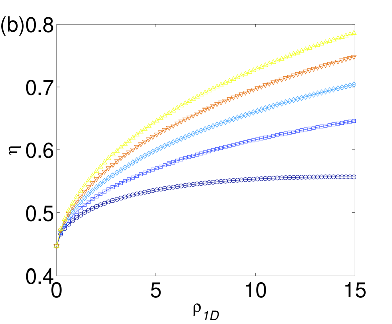
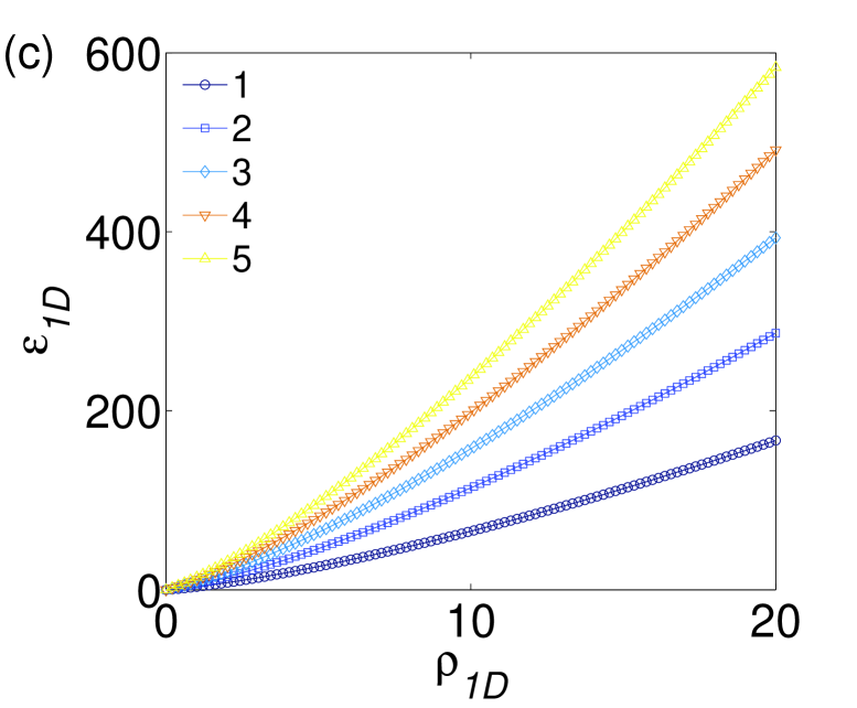
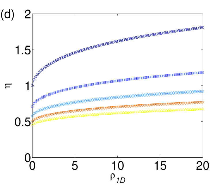
Figure 7: (a) ${\varepsilon}{{}_{\mathrm{1D}}}$ vs. ${{\rho}_{1D}}$ and (b) ${\eta}$ VS. ${{\rho}_{\mathrm{1D}}}$. In both plots the five curves correspond to ${a_{s}}/a_{c}=-0.2,-0.1,0,0.1$ and $0.2$, the confinement parameter being $\varpi_{\mathrm{t}}=5$. (c) ${\varepsilon}{{}_{\mathrm{1D}}}$ vs. ${{\rho}_{\mathrm{1D}}}$ and (d) ${\eta}$ vs. ${{\rho}_{\mathrm{1D}}}$. In both plots the five curves correspond to ${\varpi_{\mathrm{t}}}=1,2,3,4$ and $5$, and the scattering length is fixed as ${a_{s}}/a_{c}=-0.1$.

The plots in Fig. 7 show the dependence of the energy density , $\varepsilon_{\mathrm{1D}}$, and transverse width, $\eta$, on the 1D density, $\rho_{\mathrm{1D}}$, as obtained from Eqs. (28) and (30), respectively. The dependences are similar to their 2D counterparts shown in Fig. 1, i.e., the energy density increases with the atomic density, the increase being stronger at higher values of $\varpi_{\mathrm{t}}$, and with the strength of the repulsive interactions ($a_{s}>0$). The similarity is also true for the dependence of the transverse width, $\eta$, if compared to that for width, $\zeta$, in the 2D model. However, estimating the 3D density, $n_{\mathrm{3D}}$, in the case of $\rho_{\mathrm{1D}}\approx\rho_{\mathrm{2D}}$ (which also implies that $\zeta\approx\eta$), we find that the 3D density, as produced by the 1D model, is larger by a factor $\sim 1/a_{c}$. Therefore, the range of values of $n_{\mathrm{3D}}$ corresponding to Fig. 7 is much broader than in Fig. 1, implying that, using the strong 2D confinement, the unitary regime can be achieved at much lower densities than with the 1D confinement, which is explained by the fact that the Pauli-repulsion term is more important in the latter case.

Again, we assume that the gas is subject to the action of the combination of the harmonic trap and OL in the axial direction,

$${U_{\mathrm{1D}}}=\varpi_{z}^{2}{\left({Z-{Z_{0}}}\right)^{2}}+{A_{z}}{\sin^{2}}\left({{\kappa_{z}}Z}\right),$$ (32)

where $\kappa_{z}\equiv 2\pi/\lambda_{z}$ is the OL wavenumber, and $\lambda_{z}/2$ the OL period. The results obtained for such axial potentials are reported below.

4.2 The trapped quasi-1D gas in the absence of the optical lattice

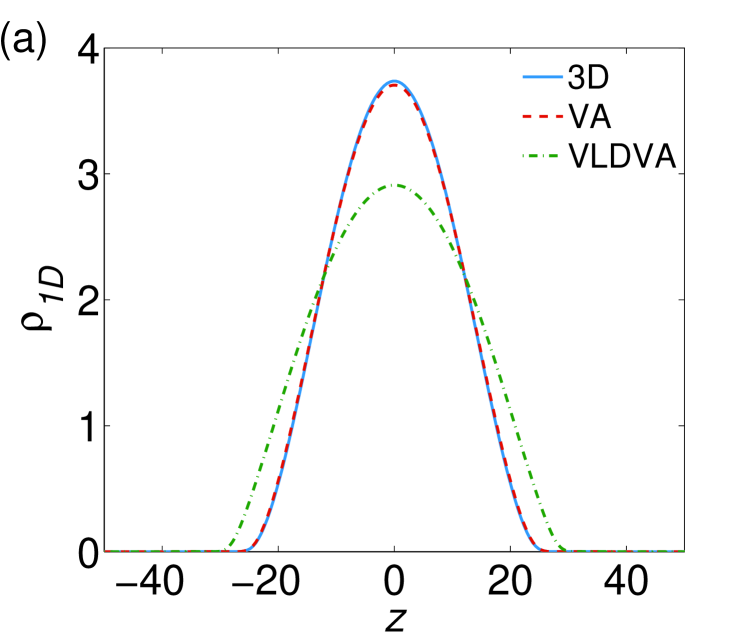
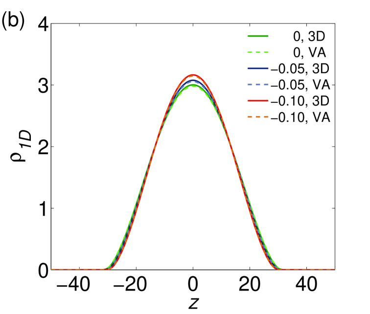
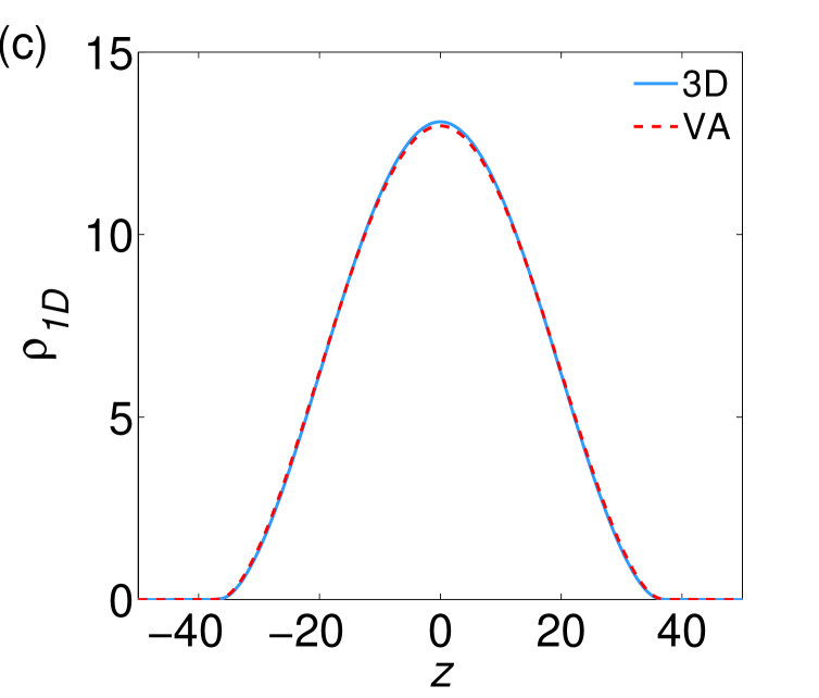
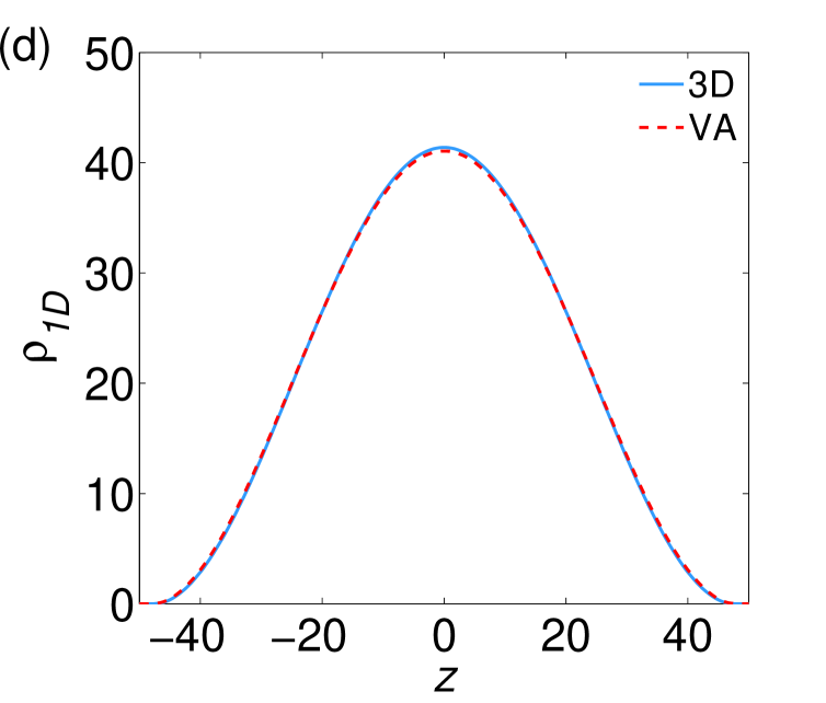
Figure 8: (Color online) The 1D density profile, $\rho_{\mathrm{1D}}$, as calculated through the full 3D solution (“3D”), and by dint of the full 1D reduction based on the variational approximate (“VA”) (panel (a) also includes the limit case of the latter, corresponding to the“very-low-density variational approximation” (“VLDVA”)). (a) Parameters are $N=100$, $a_{s}/a_{c}=0$, $\varpi_{\mathrm{t}}=1$ and $\varpi_{z}=0.1$. (b) For three values of the scattering length, $a_{s}/a_{c}=0,-0.05$ and $-0.1$, where the other parameters are $N=100$, $\varpi_{\mathrm{t}}=2$ and $\varpi_{z}=0.1$. (c) $N=500$, and (d) $N=2000$, for the other parameters $a_{s}/a_{c}=-0.05$, $\varpi_{\mathrm{t}}=2$ and $\varpi_{z}=0.1$.

As in the previous section, it is first necessary to check the accuracy of the approximation. To this end, in Fig. 8(a) we compare the 1D density, $\rho_{\mathrm{1D}}$, as produced by three different methods: the full 3D equation (7), the full 1D approximation, and its low-density limit, see Eq. (31). Similar to the 2D case, we observe an excellent agreement between the 3D equation and the full 1D approximation, both significantly disagreeing with the low-density limit. In particular, Fig. 8(b) demonstrates that the approximation remains accurate in the presence of the interactions too. On the other hand, Figs. 8(c) and (d) show that an increase in the number of atoms does not affect the agreement between the 1D and 3D simulations.

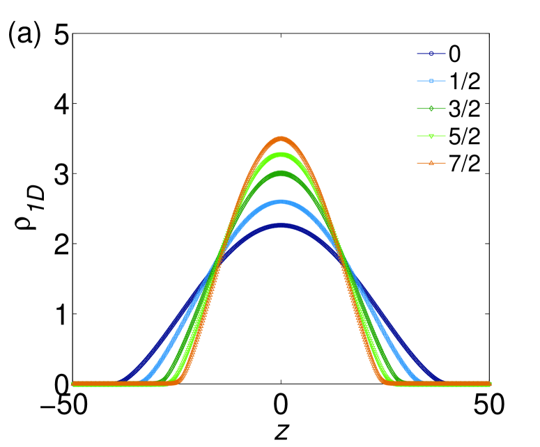
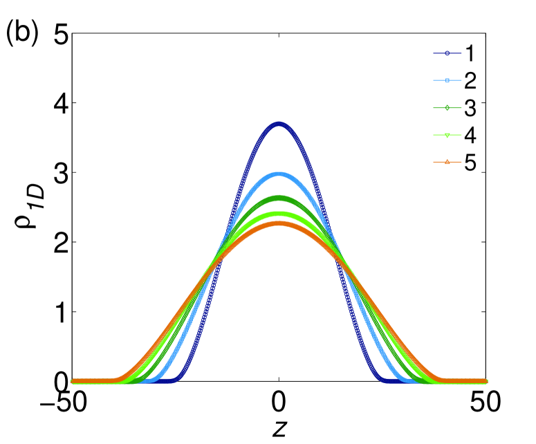
Figure 9: (Color online) (a) The 1D density profile. Five 1D density profiles correspond to $s=0,1/2,3/2,5/2$, $7/2$ (as indicated in the inset) and $\varpi_{\mathrm{t}}=5$. (b) The same, with the five curves corresponding to $\varpi_{\mathrm{t}}=1,2,3,4$, $5$ (as per the inset) and $s=0$. The parameters are $N=100$, $a_{s}/a_{c}=0$ and $\varpi_{z}=0.1$.

Figure 9(a) shows profiles of the 1D density, $\rho_{\mathrm{1D}}$, for five different values of spin $s$, in the presence of the confining harmonic-oscillator potential acting in the axial direction ($z$). The smallest width of the profile is observed at largest $s$, which is a result of the relatively weak Pauli repulsion versus the attractive interactions, as a consequence of the lower spin degeneracy. Figure 9(b) shows axial expansion of the trapped Fermi gas with the increase of the strength of the transverse confinement ($\varpi_{\mathrm{t}}$). This trend is a consequence of the rapid enhancement of the Pauli repulsion.

4.3 Effects of the axial optical lattice

Typical 1D-density patterns for the gas trapped in the OL are displayed in Fig. 10(a). Note that the increase of the confinement strength leads to attenuation of the central peak and generation of new side peaks, which is consistent with the elongation of the gas observed in Fig. 9(b). The lowering of the central peak is accompanied by the increase of the density between peaks, resulting in the reduction of their visibility. A similar behavior is observed in Fig. 10(b), where the repulsive inter-atomic interaction makes the trapped state elongated along $z$, resembling the elongation induced by the strengthening transverse confinement, and vice versa for the attractive interaction. Figure 11 shows the strong dependence of the 1D density profile $\rho_{\mathrm{1D}}$ on the OL’s (double) period $\lambda_{z}$, for a fixed strength of the confinement potential. It is clear that the number of peaks in the 1D pattern is larger for smaller $\lambda_{z}$. The increase of $\lambda_{z}$ entails disappearance of peripheral peaks at particular values of $\lambda_{z}$. The present 1D description makes it possible to identify these critical values.

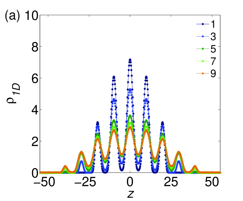
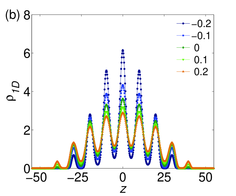
Figure 10: (Color online) One-dimensional density profiles of the Fermi gas trapped in the OL with amplitude (depth) $A_{z}=10$ and double period $\lambda_{z}=20$. (a) The five curves correspond to the confinement strength $\varpi_{\mathrm{t}}=1,3,5,7,9$ (as indicated in the top right inset). The parameters are $N=100$, $G=0$, and $\varpi_{z}=0.1$. (b) The five curves correspond to scattering lengths $a_{s}/a_{c}=0.2,0.1,0,-0.1,-02$, as indicated in the panel. The parameters are $N=100$, $\varpi_{\mathrm{t}}=5$, and $\varpi_{z}=0.1$.

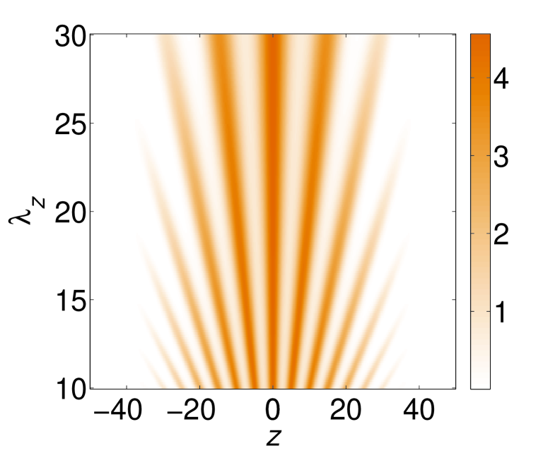
Figure 11: (Color online) One-dimensional profiles of the Fermi gas trapped in the axial optical lattice with amplitude $A_{z}=10$. The plot shows density $\rho_{\mathrm{1D}}$ versus the double lattice’s period $\lambda_{z}$. The parameters are $N=100$, $G=0$, $\varpi_{\mathrm{t}}=5$, $\varpi_{z}=0.1$.

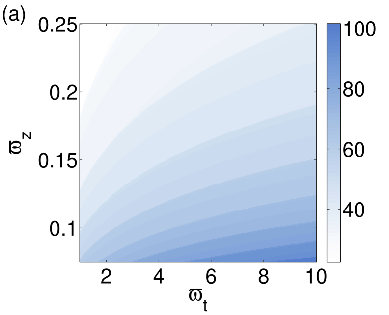
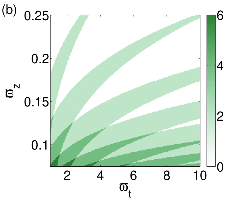
Figure 12: (Color online) Diagrams in the plane of the trapping frequencies, $\left(\varpi_{\mathrm{t}},\varpi_{z}\right)$: (a) width $\Delta_{z}$ of the area wherein $\rho_{\mathrm{1D}}>0.05$; (b) the number of density peaks at the periphery of the trapped state, which are disconnected from the central peak. The parameters are $N=100$, $a_{s}/a_{z}=-0.05$, $A_{z}=10$, $\lambda_{z}=10$.

To further analyze the ground state of the Fermi gas in presence of the OL, we define the width of the trapped state, $\Delta_{z}$, as the size of the area with density $\rho_{\mathrm{1D}}>0.05$. Figure 12 presents diagrams for characteristics of the ground state in the plane of the transverse and axial trapping frequencies, $\left(\varpi_{\mathrm{t}},\varpi_{z}\right)$. The jumps observed in Fig. 12(a) correspond to the emergence or disappearance of pairs of density peaks. Since the wavelength is $\lambda_{z}=10$, the emergence or disappearance of the peak pair gives rise, respectively, to the increase or decrease of the width by $\Delta_{z}=10$. Thus, the observed minimum width ($\Delta_{z}=20$) corresponds to the profile with five peaks, and the maximum width ($\Delta_{z}=110$) is represented by the profile with twenty three peaks. Note that, as seen in Fig. 10, the density between peaks may be very small.

Further, we define that two peaks as being “connected” if the minimum density between them is greater than $0.05$. Accordingly, Fig. 12(b) shows the number of peaks “disconnected” from the central core. This characteristic is found by subtracting the number of the connecting links between the peaks, defined as said above, from the total number of the observed peaks (excluding the central one). The diagram features four regions covered by similar colors, which correspond to four possible values of the number of isolated peaks, $0,2,4$ and $6$. These regions alternate with the variation of both $\varpi_{\mathrm{t}}$ and $\varpi_{z}$, demonstrating that the number of the isolated peaks may be maintained while varying the total number of the observed peaks.

5 Conclusions

We have demonstrated that the 1D and 2D reductions of the 3D mean-field description of the degenerate Fermi gas, based on the Gaussian variational ansatz, provide very accurate results for the ground states of the gas in the disk- and cigar-shaped traps. The so derived reduced equations are useful, in particular, for modeling the BCS regime at low atomic density and large spatiotemporal variations of the external potential. For the 1D case, the reduced equations provide results requiring the use of modest computational resources and allow one to quickly explore a vast volume of the parameter space. In the 2D case, the necessary simulation time is still significantly lower than what is necessary for the 3D simulations. For the spatially uniform ground states in both dimensions, we have studied the width of the Fermi gas in the confinement dimensions, and the energy density as a function of the atomic density. In the 2D case, we have found that the energy density attains a maximum at a particular value of the atomic density, and the maximum shifts to lower values as the attractive interactions get stronger. While the analysis is approximate due to limitations of the model, it shows the correct dependence on the scattering length, confinement strength, and the phase-space degeneracy (i.e., the fermionic spin, $s$).

For the gas trapped in the 2D OL, the analysis predicts the number of visible peaks in the density profile as a function of the scattering length and confinement strength. It was concluded that small variations of the latter parameter produce significant changes in the size and distribution of the peaks. In the 1D setting including the axial OL, we have produced the phase diagrams for the Fermi gas, varying the confinement parameters. Discrete leaps in the diagrams correspond to the appearance and disappearance of a pair of peripheral peaks in the density profile. In fact, the number of peaks does not change in a wide range of the confinement parameters.

In general, our model is able to include any type of the confinement and potential lattices in the 1D and 2D settings, making the description of the ground state quite simple. In particular, we considered the example of the hexagonal superlattice built as a superposition of two triangular lattices. The latter setting may be essential for modeling configurations relevant to solid-state physics. The same approach may be further applied to superlattices built of hexagonal OLs, with the objective to emulate graphene-like superlattice. Beyond the study of the ground states, it may be interesting to build quasi-2D modes with embedded vorticity, cf. Ref. [24]. On the other hand, the reduced equations can be used to study the dynamics of the Fermi gas under the action of external potentials slowly varying in time, similar to how it was done in BEC models. Finally, the same type of the description, including, if necessary, equations for the Bose gas, may be used to predict the ground state and analyze the low-energy dynamics of Fermi-Fermi and Bose-Fermi mixtures.

References

References

- [1] Bongs K and Sengstock K 2004 Rep. Prog. Phys. 67 907
- [2] Jaksch D and Zoller P 2005 Ann. Phys. 315 52
- [3] Lewenstein M Sanpera A Ahufinger V Damski B Sen (De) A and Sen U 2007 Adv. Phys. 56 243
- [4] Giorgini S Pitaevskii L P and Stringari S 2008 Rev. Mod. Phys. 80 1215; Bloch I Dalibard J and Zwerger W 2008 Rev. Mod. Phys. 80 885
- [5] Kartashov Y V Malomed B A and Torner L 2011 Rev. Mod. Phys. 83 247
- [6] Snoek M Titvinidze I Bloch I and Hofstetter W 2011 Phys. Rev. Lett. 106 155301;
- [7] Fröhlich B Feld M Vogt E Koschorreck M Zwerger W and Koḧl M 2011 Phys. Rev. Lett. 106 105301
- [8] Tempere J and Devreese J T 2006 J. Phys. B: At. Mol. Opt. Phys. 39 S57
- [9] Paananen T 2009 J. Phys. B: At. Mol. Opt. Phys. 42 165304
- [10] Adhikari S K 2010 J. Phys. B: At. Mol. Opt. Phys. 43 085304
- [11] Watanabe G Dalfovo F Pitaevskii L P and Stringari S 2011 Phys. Rev. A 83 033621
- [12] Snoek M Titvinidze I and Hofstetter W 2011 Phys. Rev. B 83 054419
- [13] Adhikari S K 2006 Phys. Rev. A 73 043619
- [14] Hu H Liu X J and Drummond P D 2007 Phys. Rev. Lett. 98 070403
- [15] Giraud S and Combescot R 2009 Phys. Rev. A 79 043615
- [16] Blume D and Rakshit D 2009 Phys. Rev. A 80 013601
- [17] Bertania G and Giorgini S 2009 Phys. Rev. A 79 013616
- [18] Jackson A D Kavoulakis G M and Pethick C J 1998 Phys. Rev. A 58 2417
- [19] Kim Y A and Zubarev A L 2004 Phys. Rev. A 70 033612
- [20] Capuzzi P and Vignolo P 2008 Phys. Rev. A 78 043613
- [21] Lieb E H and Liniger W 1963 Phys. Rev. 130 1605; Lieb E H Phys. Rev. 130 1616
- [22] M. Gaudin 1967 Phys. Lett. 24A 55; Yang C N 1967 Phys. Rev. Lett. 19 1312
- [23] Fuchs J N Recati A and Zwerger W 2004 Phys. Rev. Lett. 93 090408
- [24] Adhikari S and Malomed B A 2007 Europhys. Lett. 79 50003; 2009 Physica D 238 1402
- [25] Adhikari S K and Malomed B A 2006 Phys. Rev. A 74 053620
- [26] Adhikari S K 2007 Phys. Rev. A 76 053609
- [27] Salasnich L Parola A and Reatto L 2002 Phys. Rev. A 65 043614
- [28] Salasnich L and Malomed B A 2009 Phys. Rev. A 79 053620
- [29] von Weizsäcker C F 1935 Z. Phys. 96 431
- [30] Kirzhnitz D A Field Theoretical Methods in Many-Body Systems (Pergamon Press, London 1967)
- [31] Huang K and Yang C N 1957 Phys. Rev. 105 767, ibid. 105 1119
- [32] Tey M K Stellmer S Grimm R and Schreck F 2010 Phys. Rev. A 82 011608
- [33] Kim Y E and Zubarev A L 2004 Phys. Rev. A 69 023602
- [34] Adhikari S K 2007 Phys. Rev. A 76 023612
- [35] Chen Q He Y Chien C-C and Levin K 2006 Phys. Rev. A 74 063603