Solving the Graph Isomorphism Problem with a Quantum Annealer

Abstract

We propose a novel method using a quantum annealer – an analog quantum computer based on the principles of quantum adiabatic evolution – to solve the Graph Isomorphism problem, in which one has to determine whether two graphs are isomorphic (i.e., can be transformed into each other simply by a relabeling of the vertices). We demonstrate the capabilities of the method by analyzing several types of graph families, focusing on graphs with particularly high symmetry called strongly regular graphs (SRG’s). We also show that our method is applicable, within certain limitations, to currently available quantum hardware such as “D-Wave One”.

I Introduction

Theoretical research on quantum computing is motivated by the exciting possibility that quantum computers may be able to perform certain tasks faster than classical computers. In recent years first steps have been taken towards the goal of experimentally realizing these computational advantages. However, to date the largest experimental implementations of scientifically meaningful quantum algorithms have used just a handful of qubits  Vandersypen et al. (2001); Bian et al. (2012), the reason being the tremendous technological challenges (the most crucial of which is overcoming quantum decoherence) that need to be defeated before a successful implementation of any solid-state quantum computer.

Of the several quantum computing paradigms that have been proposed, a potentially promising substitute for the ‘standard’ circuit-based quantum computer is the quantum annealer Kadowaki and Nishimori (1998); Farhi et al. (2001a), which is now on the cusp Bian et al. (2012) of being able to run small-scale computing procedures on actual quantum annealing hardware. Quantum annealing machines are analog quantum computational devices designed to solve discrete combinatorial optimization problems using properties of quantum adiabatic evolution. They are based on a general approach widely known as the Quantum Adiabatic Algorithm (QAA), which was proposed by Farhi et al. Farhi et al. (2001b) about a decade ago as a method for solving a broad range of optimization problems using a quantum computer.

Recently, a quantum annealing machine, based on liquid crystal nuclear magnetic resonance has been reported to successfully factor the number $143$ using four spin-qubits Xu et al. (2011). A few months later, “D-Wave One”, a $128$-qubit machine based on super-conducting qubits Johnson et al. (2011) experimentally demonstrated the ability to compute two-color Ramsey numbers Gaitan and Clark (2012); Bian et al. (2012) making it the largest experimental implementation of a scientifically meaningful quantum algorithm. This success provides an incentive for finding problems that could be solved efficiently on a quantum annealer.

In this paper, we hypothesize that a quantum annealer could solve the Graph Isomorphism (GI) problem, described in detail below. In particular, we hypothesize that the annealer could distinguish all non-isomorphic graphs by sufficiently precise measurements. We provide some evidence for this by showing that our method works for certain graphs which we have been able to study numerically. An advantage of our proposal is that it can, within certain limitations, be implemented using currently available quantum annealing machines such as D-Wave One.

The paper is organized as follows. In Sec. II we describe the Graph Isomorphism (GI) problem in some detail. In Sec. III we describe and then discuss the proposed method for solving the GI problem using quantum adiabatic evolution. We next present the results of the study in Sec. IV and derive some conclusions in Sec. V.

II The Graph Isomorphism Problem

A graph $G=(V,E)$ is a set of vertices $V$, and edges $E$ which are unordered pairs of vertices. A graph is conveniently expressed algebraically as an adjacency matrix. The adjacency matrix $A$ of a graph with $N$ vertices is an $N\times N$ matrix in the basis of vertex labels, with $A_{ij}=1$ if vertices $i$ and $j$ are connected by an edge, and zero otherwise.

The GI problem is stated as follows: Given two graphs, one must determine whether or not they are isomorphic to each other, i.e., whether one can be transformed into the other by a relabeling of the vertices.

In the realm of classical computing, many special cases of GI have been shown to be solvable in a time that scales as a polynomial of the number of vertices. However the best general algorithm to date runs in time $\mathcal{O}\left(a^{N^{1/2}\log N}\right)$ where $a$ is a constant Spielman (1996). It is therefore interesting to ask whether a quantum computer could solve this problem efficiently. An attractive feature of the GI problem is its resemblance to the problem of integer factoring, the first and most famous example to date of a quantum algorithm can solve a problem exponentially faster than the best known classical algorithm Shor (1994). Like factoring, the common belief is that the GI problem is unlikely to be NP-complete.

The GI problem has been attacked by numerous methods inspired by classical as well as quantum physical systems. Rudolph Rudolph (2002) mapped the GI problem onto a system of hard-core atoms, where one atom was used per vertex, and atoms $i$ and $j$ interacted if vertices $i$ and $j$ were connected by edges. It was demonstrated that for some pairs of non-isomorphic graphs, sharing cospectral adjacency matrices does not lead to cospectrality of the transition matrix between three-particle states produced by the embedded Hamiltonian. Gudkov and Nussinov Gudkov and Nussinov (2002) proposed a classical algorithm to distinguish non-isomorphic graphs by mapping them onto various physical problems. Shiau et al. proved that the simplest classical algorithm fails to distinguish some pairs of non-isomorphic graphs and also proved that continuous-time one-particle quantum random walks cannot distinguish some non-isomorphic graphs Shiau et al. (2005); Gamble et al. (2010); Rudinger et al. (2012). More recently, it has been found that classical random walks and quantum random walks can exhibit qualitatively different properties Aharonov et al. (1993); Bach et al. (2004); Solenov and Fedichkin (2006). These disparities mean that in some cases algorithms implemented by quantum random walkers can be proven to run faster than the fastest possible classical algorithm Childs et al. (2002); Shenvi et al. (2003); Ambainis (2003, 2004); Magniez et al. (2007); Potoc̆ek et al. (2009); Reitzner et al. (2009); Douglas and Wang (2008); Emms et al. (2006, 2009).

III Quantum Adiabatic Evolution and the GI Problem

To solve the GI problem using quantum adiabatic evolution, we assign to each graph $G$ the Hamiltonian $\hat{H}(G)$, where

$$\hat{H}(G)=(1-s)\hat{H}_{d}+s\hat{H}_{p}(G)\,,$$ (1)

which depends on a parameter $s$. For $s=0$, $\hat{H}(G)$ is the standard ’driver’ Hamiltonian for QAA algorithms, namely

$$\hat{H}_{d}=\frac{1}{2}\sum_{i}^{N}\sigma_{i}^{x},$$ (2)

i.e., a transverse-field Hamiltonian, while for $s=1$, $\hat{H}(G)$ is the ’problem’ Hamiltonian $\hat{H}_{p}(G)$ which is constructed according to the topology of the graph. A simple plausible choice for $\hat{H}_{p}(G)$ is

$$\hat{H}_{p}(G)=\sum_{\langle ij\rangle\in G}\sigma_{i}^{z}\sigma_{j}^{z}\,,$$ (3)

i.e., an Ising antiferromagnet on the edges of the graph. While the driver Hamiltonian is diagonal in the $\prod\sigma^{x}$ basis, the problem Hamiltonian is diagonal in the $\prod\sigma^{z}$ basis.

The system is first prepared in the ground state of the driver Hamiltonian $\hat{H}_{d}$, which is straightforward. The adiabatic parameter $s$ is then varied slowly and smoothly with time from $0$ to $1$, so that the Hamiltonian is continuously modified from $\hat{H}_{d}$ to $\hat{H}_{p}(G)$. If this process is done slowly enough, the adiabatic theorem of Quantum Mechanics (see, e.g., Refs. Kato (1951) and Messiah (1962)) ensures that the system will stay close to the ground state of the instantaneous Hamiltonian throughout the evolution.

The premise of the method we suggest here is that the state of the system along the adiabatic evolution, i.e., the instantaneous ground state of the Hamiltonian, Eq. (1), stores enough information to reflect the complex structure of the graph-dependent problem Hamiltonian $\hat{H}_{p}(G)$, and that carefully chosen measurements along the adiabatic path will provide enough information to differentiate non-isomorphic graphs.

The choice of the problem Hamiltonian in Eq. (3) is, of course, only one possibility. However it has the advantages of (i) using Ising spins which are simple to study and to implement experimentally Johnson et al. (2011); Bian et al. (2012), and (ii) having antiferromagnetic interactions which, on highly-connected graphs, tend to have highly frustrated ground-states because closed paths (along the edges) of odd length make the system a spin glass Mézard and Parisi (2001, 2003); Zdeborová and Boettcher (2010); Farhi et al. (2012). Note also, that the Hamiltonian Eq. (1) is symmetric with respect to flipping all spins.

It is interesting to compare our approach with those which use Hamiltonians of quantum random walkers embedded in the graph structure. In the latter case the walker normally accesses only low-dimensional subspaces of the Hamiltonian eigenstates, based on conserved quantities such as number of particles (see, e.g., Refs. Rudolph (2002); Shiau et al. (2005); Emms et al. (2006, 2009)), whereas in our approach there is no such conserved quantity so the instantaneous ground state of the Hamiltonian presumably reflects the full complexity of the graph.

For each graph, one performs multiple runs along the adiabatic path, performing various measurements at different values of $s$ until sufficient statistics is gathered. Since each measurement collapses the state of the system, non-commuting measurements or measurements corresponding to different $s$ values, require separate runs of the procedure. Since errors of the various measured quantities are inversely proportional to square root of the number of measurements, this number will be determined from the needed resolution.

In order to make sure that isomorphic graphs are recognized as such, the measurements must be invariant under a relabeling of the vertices of the graph (or equivalently the spins in the system). The most straightforward such quantity is the Hamiltonian, so the average energy $E=\langle\hat{H}(G)\rangle$ is a ‘good’ quantity to measure. Here, $\langle\cdot\rangle$ indicates the expectation value with respect the state of the system, i.e., the instantaneous ground-state, at a particular value of $s$. For the same reason, the classical ‘diagonal’ average energy of the graph $E_{G}=\langle\hat{H}_{p}(G)\rangle$ and $M_{x}=2\langle\hat{H}_{d}\rangle$, the $x$-magnetization, are also suitable observables.

Many other quantities that respect the topology of the graph and are invariant under any relabeling of the vertices could be measured. Some may prove to have better distinguishing capabilities than others, depending on the manner in which they ‘tap’ into the complexity of the structure of the graph in question.

We find that a ‘good’ quantity to measure is the spin-glass order parameter, which we shall denote as $Q_{2}$ and define by

$$Q_{2}=\left({1\over N(N-1)}\,\sum_{i\neq j}\langle\sigma_{i}^{z}\sigma_{j}^{z}\rangle^{2}\right)^{1/2}\,.$$ (4)

Generalizing the above expression, the quantities

$$Q_{2n}=\frac{1}{N^{2n}}\sum_{i_{1},i_{2},\ldots,i_{2n}}\langle\sigma_{i_{1}}^{z}\sigma_{i_{2}}^{z}\ldots\sigma_{i_{2n}}^{z}\rangle^{2}\,,$$ (5)

where $n=2,3,4\ldots$, also serve as distinguishing operators. Analogously, other types of operators that might work are of the form:

$$Q_{2}^{\prime}=\frac{1}{N^{2}}\sum_{i,j}\langle\hat{H}_{p}(G)\sigma_{i}^{z}\sigma_{j}^{z}\rangle^{2}\,.$$ (6)

Each such measurable quantity, if measured sufficiently accurately, for different values of the adiabatic parameter $s$, serves as an additional ‘dimension’ of differentiability of the non-isomorphic graphs. Moreover, gathering statistics of these quantities for different values of $s$ accesses indirectly the entire spectrum of $\hat{H}_{p}(G)$ (unlike the situation in classical or quantum random walks where the walkers are restricted to only a small subspace of the Hamiltonian eigenstates).

In Sec. IV we will consider several sets of non-isomorphic graphs, showing that, in all cases, non-isomorphic graphs are distinguished by accurate measurements of carefully chosen observables along the adiabatic path. In fact, we shall see that in most cases studying the limit $s\to 1$ suffices.

IV Results

We now present numerical and semi-analytical results for several types of graph families that are known to be hard to distinguish. Since the annealing process requires that the temperature of the system be well below the excitation gap of the system, we shall work at zero temperature.

For the smaller graphs that we study ($N\leq 25$ vertices), we use exact-diagonalization or conjugate-gradient based minimization techniques. Both techniques are restricted to quite small values of $N$ because the size of the Hilbert space grows as $2^{N}$. The specific variation of conjugate-gradient method that we developed for this study is discussed in Appendix A.

For graphs of more than $25$ vertices, quantum Monte-Carlo techniques would usually be the method of choice for the accurate measurements of the various quantities. However, these were found by us to be rather inefficient in the interesting regions where the value of the adiabatic parameter is close to $1$. We have been able to study sizes a little larger than $25$ (up to $29$) by leading-order degenerate perturbation theory about the limit $s=1$. This calculation involves finding the subspace of ground states of $\hat{H}_{p}(G)$, which requires one to first calculate the energies of the $2^{N}$ ‘classical’ states followed by further manipulation on the subspace spanned by the ground-state eigenvectors. The main shortcoming of the method is that it only produces results in the $s\to 1$ limit. Fortunately, we find that in most cases this is sufficient.

The measured quantities we focus on are the total (average) energy, the spin-glass order parameter $Q_{2}$ given in Eq. (4) and the $x$-magnetization $M_{x}=2\langle\hat{H}_{d}\rangle$. We find that in most cases these three quantities are sufficient to distinguish all tested non-isomorphic graphs, though these measurements may be augmented by measuring other observables, as discussed in the previous section.

IV.1 Strongly regular graphs

The main results of this paper are for strongly regular graphs (SRGs), a class of graphs, subsets of which are known to be difficult to distinguish Gamble et al. (2010). An SRG is a graph in which (i) all vertices have the same degree, (ii) each pair of neighboring vertices has the same number of shared neighbors, and (iii) each pair of non-neighboring vertices has the same number of shared neighbors. This definition permits SRGs to be categorized into families by four integers $(N,k,\lambda,\mu)$, each of which might contain many non-isomorphic members. Here, $N$ is the number of vertices in each graph, $k$ is the degree of each vertex (k-regularity), $\lambda$ is the number of common neighbors shared by each pair of adjacent vertices, and $\mu$ is the number of common neighbors shared by each pair of non-adjacent vertices.

Using the stringent constraints placed on SRGs, one can show that, for any SRG, the spectrum of the adjacency matrix has only three distinct values Godsil and Royle (2001): $\lambda_{0}=-k$, which is non-degenerate, and $\lambda_{1,2}=-\frac{1}{2}\left(\lambda-\mu\pm\sqrt{N}\right)$, which are both highly degenerate. Both the value and degeneracy of these eigenvalues depend only on the family parameters, so within a particular SRG family, all graphs are cospectral Godsil and Royle (2001). These highly degenerate spectra are one reason why distinguishing non-isomorphic SRGs is difficult.

While there exist SRG families with only one non-isomorphic member Weisstein , we concern ourselves with families that have more than one non-isomorphic graph. Using combinatorial techniques Spence ; McKay , tables of complete and partial families of SRGs have been tabulated and we will use those tables to select graphs for our study. It should be noted that for every family of non-isomorphic SRGs there exists a complementary family of the same size $N$ and the same number of members, which is obtained by interchanging edges and non-edges.

The smallest family of non-isomorphic SRGs that have more than one member is that of the $N=16$ vertices with signature $(16,6,2,2)$, which contains two members (we shall not address here the complementary families of graphs which are distinguished in much the same way). The two graphs are immediately distinguished by looking for example at the spin-glass order parameter $Q_{2}$ as a function of the adiabatic parameter $s$. The $Q_{2}$ values of the two graphs (at zero temperature) are plotted as a function of $s$ in Fig. 1. In this $N=16$ case, both graphs have the same ‘classical’ ground-state energy of $E_{G}=\langle\hat{H}_{p}(G)\rangle=-16$ albeit with different degeneracies, namely $21$ and $45$ bit .

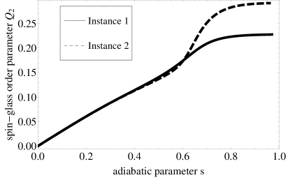
Figure 1: Spin-glass order parameter $Q_{2}$ in the ground state for the two non-isomorphic strongly-regular graphs (SRGs) on $N=16$ vertices. As the figure indicates, the two graphs show different $Q_{2}$ values starting from $s\simeq 0.4$.

The next family of SRGs that contains more than one member is that with $N=25$ vertices. This family has $15$ distinct graphs with signature $(25,12,5,6)$. We find that looking at the values of $Q_{2}$ and $M_{x}$ in the ground state in the limit of $s\to 1$ using first-order degenerate perturbation theory suffices to distinguish between all but two of the graphs (the latter two share the same $Q_{2}$ and $M_{x}$ values in this limit). The results are shown in Fig. 2, which is a scatterplot of $Q_{2}$ vs $M_{x}$ for $s\to 1$ for all 15 non-isomorphic graphs. In this limit, most instances have the same ground-state energy of $E_{G}=-34$ except for two instances which have a slightly higher energy of $E_{G}=-30$. These correspond to the two points in the inset of Fig. 2. In addition, the circled data point in the figure corresponds to the $(M_{x},Q_{2})$ value of the two graphs which are not distinguished in the $s\to 1$ limit. However, for values of $s$ less than 1, exact diagonalization reveals a clear distinction between the two graphs. For example, for $s=0.73$ the values of $Q_{2}$ in the ground state are $0.57914$ and $0.443423$.

Figure 2: Scatterplot in the $M_{x}-Q_{2}$ plane of the $15$ strongly regular graphs with $N=25$ vertices in the limit $s\to 1$. The horizontal axis is the magnetization along the $x$-direction and the vertical axis is the spin-glass order parameter $Q_{2}$. The circled data point corresponds to the only two graphs which are not distinguished by values of $Q_{2}$ and $M_{x}$ in the $s\to 1$ limit. These two instances are, nonetheless, distinguished by measurements at $s<1$ (see text). The inset shows the $M_{x}-Q_{2}$ values of two of the graphs that lie outside of the region shown in the main panel.

Perturbation theory-based analysis in the $s\to 1$ limit also allows us to study families of graphs with $N=26,28$ and $29$ vertices. The degenerate perturbation-theory analysis of the set of $10$ SRGs with $N=26$ and signature $(26,10,3,4)$ are shown in Fig. 3 which is a scatterplot in the $M_{x}-Q_{2}$ plane. Here, 7 of the instances were found to have $E_{G}=-34$ (with different degeneracies, all of them around $\sim 1000$) and required first-order perturbation theory, whereas the remaining 3 instances had $E_{G}=-38$ (with degeneracies $20,20$ and $60$), and the leading-order perturbation analysis is of degree 6. Fig. 3 shows that all 10 members of the family are distinguished in that plane. The inset shows data points that lie outside of the range presented in the main panel.

Figure 3: Scatterplot in the $M_{x}-Q_{2}$ plane of the $10$ strongly regular graphs with $N=26$ vertices and signature $(26,10,3,4)$, in the $s\to 1$ limit. As the figure indicates, the annealer distinguishes all graphs in the family.

For $N=28$, the family $(28,12,6,4)$ contains $4$ distinct graphs. There too, we find that it is sufficient to look at the $Q_{2}$ values and average total energy in the $s\to 1$ limit. For three of the four graphs that have the ground-state energy of $E_{G}=-28$ (and with different degeneracies, all of them around $\sim 6000$) the $Q_{2}$ values are $0.137461$, $0.141957$ and $0.132883$. The fourth graph has a different energy of $E_{G}=-24$ (with a degeneracy of $972265$). The $Q_{2}$ value has not been calculated for this graph.

The largest size of graphs that we deal with analytically using perturbation theory is the family of $41$ graphs having $N=29$ vertices and signature $(29,14,6,7)$. A scatterplot in the $M_{x}-Q_{2}$ plane for this family is given in Fig. 4. While some of the values shown in the scatterplot lie close to one another, all pairs $(M_{x},Q_{2})$ are distinct (and can be further differentiated by measurements of other observables) so all non-isomorphic graphs of this family can be distinguished. Here, all members were found to have the same energy of $E_{G}=-41$ and with different degeneracies, all of them around $\sim 3000$.

Figure 4: Scatterplot in the $M_{x}-Q_{2}$ plane of the $41$ strongly regular graphs with $N=29$ vertices, in the $s\to 1$ limit. As the figure indicates, the annealer distinguishes all graphs in the family. The inset shows data points that are out of the range presented in the main panel.

IV.2 Other pairs of graphs

Strongly-regular graphs are only one of many classes of graphs that are considered difficult to distinguish. Here, we discuss two regular (rather than strongly-regular) pairs of graphs that are known to be difficult to distinguish (and were, in fact, constructed to be so). The first pair, which we denote here as ($G_{1}$,$G_{2}$) was first considered by Emms et al. Emms et al. (2006, 2009) (the reader is referred Appendix B for the adjacency matrices of the two graphs). The two graphs are regular having 14 vertices. They were given as an example of non isomorphic graphs that can not be distinguished by certain quantum random walkers, although it should be noted that other more recent quantum random walkers seem to be able to distinguish between the graphs ken .

While having almost identical adjacency matrices and therefore also almost identical energies and $Q_{2}$ values for $s\to 1$, the two graphs can still be distinguished by our quantum annealer, at least within a small region of $s$. This can be seen by looking at differences in $Q_{2}$ values (and smaller but visible differences in the energy). These are shown in Fig. 5. Interestingly, this region precisely corresponds to the quantum phase transition normally seen in quantum adiabatic computing procedures that is characterized by a small gap Young et al. (2008, 2010). This region is therefore the usual ‘bottleneck’ of the Quantum Adiabatic Algorithm.

Figure 5: The difference in $Q_{2}$ values, $\Delta Q_{2}$ (main panel) and energies (inset), for the two graphs $G_{1}$ and $G_{2}$ with $N=14$ that certain quantum walkers cannot distinguish Emms et al. (2006, 2009).

We also considered another pair of non-isomorphic regular graphs on 16 vertices, denoted here by $G_{3}$ and $G_{4}$ (the reader is referred Appendix B for the adjacency matrices of the two graphs), that are known to be difficult to distinguish Godsil and Royle (2001); Guo (2010). Similarly to the previous pair ($G_{1}$,$G_{2}$), the pair ($G_{3}$,$G_{4}$) can be distinguished by looking at the $Q_{2}$ and energy differences as a function of $s$, see Fig. 6.

Figure 6: The difference in $Q_{2}$ values, $\Delta Q_{2}$ (main panel) and energies (inset), for the two graphs $G_{3}$ and $G_{4}$ with $N=16$ that certain quantum walkers cannot distinguish Guo (2010).

Interestingly, if one inspects the spectra of the ‘diagonal’ Hamiltonians $\hat{H}_{p}(G)$ of the two pairs of graphs, one finds that each pair shares the exact same spectrum, meaning that while ‘classically’ it is impossible to distinguish between the graphs within each pair, extending the analysis to the ‘quantum region’, by adding a non-commuting term (the driver Hamiltonian) enables the crucial missing differentiation.

V Conclusions and Future Research

The results we presented here support a conjecture that the Quantum Adiabatic prescription can differentiate between all non-isomorphic graphs, given an appropriate choice of problem and driver Hamiltonians. This conjecture needs to be tested more thoroughly, both theoretically and also by experiments on real quantum annealers.

In future studies, it would be desirable to study larger examples of SRG’s, and also consider other types of graphs such as the Cai, Fürer and Immerman graph constructions Cai et al. (1989), which are too large to be studied with the methods used here and would require Quantum Monte Carlo simulations.

In the current study we have distinguished between graphs by measurements of average quantities like $M_{x}=\langle\sum_{i}\sigma^{x}_{i}\rangle$ (i.e., magnetization along the $x$-direction) and $\sum_{i\neq j}\langle\sigma^{z}_{i}\sigma^{z}_{j}\rangle^{2}$. More information would be obtained by more sophisticated analyses of measurement data. One example, would be to calculate higher moments of the obtained data rather than using only averages as we have done in this study. Another example would be comparing the individual (sorted) values rather than the average over sites far . This should be done in future studies.

It is important to understand the efficiency of the algorithm we propose, i.e. how the running time of the algorithm scales with graph size for large sizes. This requires an analysis of the size dependence of the minimum gap for large sizes, presumably using Quantum Monte Carlo simulations, e.g. Hen and Young (2011), to get to large enough sizes to see the trend.

An attractive feature of the method proposed here is that it can be implemented in principle by existing (albeit prototypical) quantum annealers. We require a quantum annealer that has Ising-spin interactions of finite connectivity plus constant transverse magnetic fields. The prototypical “D-Wave One” machine Johnson et al. (2011) has these capabilities. However, D-Wave One can not calculate the quantities studied here, $\langle\sigma^{x}_{i}\rangle$ and $\langle\sigma^{z}_{i}\sigma^{z}_{j}\rangle$, though it can calculate averages of a single $\sigma^{z}$ and also susceptibilities involving $\sigma^{z}$ ami . For the model studied here, $\langle\sigma^{z}_{i}\rangle$ is zero because of the bit-flip symmetry of the Hamiltonian. However, one could break this symmetry by adding a field coupling to $\sigma^{z}$ and use the values of the $\langle\sigma^{z}_{i}\rangle$ to distinguish between graphs. In other words, it seems likely to us that quantities which D-Wave One can calculate would also be useful for the Graph Isomorphism problem. Another useful quantity which can be determined by D-Wave hardware ami is the distribution of the energy as a function of the evolution time of the algorithm. This distribution would be sensitive to the details of spectrum of the graph and is therefore also likely be a good discriminant between graphs.

Appendix A Conjugate gradient method

In this appendix we explain the version of the conjugate-gradient method that was used in this study to calculate the ground state of a given Hamiltonian. We found that the ‘traditional’ Lanczos and conjugate-gradient methods are not sufficiently accurate for our problem, so we had to develop a new variant of these methods.

The ground state of a Hamiltonian $\hat{H}$ is obtained by minimizing

$$E_{0}=\min f(|\psi\rangle)=\min_{\{|\psi\rangle\}}\frac{\langle\psi|\hat{H}|\psi\rangle}{\langle\psi|\psi\rangle}\,.$$ (7)

The key feature is that the objective function $f$ has no local minima but only the one global minimum that we need. Hence, in principle, any minimization method would work, but we find that this is not the case in practice because of the limitations of finite-precision arithmetic. After choosing a basis $\{|n\rangle\}$, one can write $|\psi\rangle=\sum c_{n}|n\rangle$, and the objective function to be minimized becomes

$$E_{0} = \min f(\{c_{n}\})$$

$$= \min_{\{c_{n}\}}\frac{\sum_{n}c_{n}^{2}d_{n}+\sum_{n}c_{n}\sum_{m}a_{nm}c_{m}}{\sum_{n}c_{n}^{2}}\,,$$

in which we denote the diagonal elements of the Hamiltonian by $\hat{H}_{nn}=d_{n}$ and the off-diagonal elements (presumably sparse) by $\hat{H}_{nm}=a_{nm}$. In what follows we shall assume that the coefficients $c_{n}$ are real-valued for convenience. The generalization to complex-valued coefficients is trivial.

The basic conjugate gradient method in this case is very simple. Firstly, the gradient with respect to the various parameters $c_{n}$ is easily obtainable:

$$\frac{\partial f}{\partial c_{k}} = \frac{2d_{k}c_{k}+2\sum_{m}a_{km}c_{m}}{\sum_{n}c_{n}^{2}}$$

$$- \frac{2c_{k}\left(\sum_{n}c_{n}^{2}d_{n}+\sum_{n}c_{n}\sum_{m}a_{nm}c_{m}\right)}{\left(\sum_{n}c_{n}^{2}\right)^{2}}\,.$$

Secondly, the one-dimensional minimization steps of the conjugate gradient method can be calculated explicitly

$$\min_{\alpha} f(|\psi\rangle+\alpha|\delta\rangle)=$$

$$\min_{\alpha} \frac{\langle\delta|\hat{H}|\delta\rangle\alpha^{2}+2\operatorname{Re}\langle\psi|\hat{H}|\delta\rangle\alpha+\langle\psi|\hat{H}|\psi\rangle}{\langle\delta|\delta\rangle\alpha^{2}+2\operatorname{Re}\langle\psi|\delta\rangle\alpha+\langle\psi|\psi\rangle}\,.$$

The above expression is minimized for $\alpha=\alpha*$ which is one of the two solutions of a quadratic equation, and this produces the minimum (along the line) energy of:

$$E_{0} = f(|\psi\rangle+\alpha^{*}|\delta\rangle)$$

$$= \frac{\langle\delta|\hat{H}|\delta\rangle{\alpha^{*}}^{2}+2\operatorname{Re}\langle\psi|\hat{H}|\delta\rangle\alpha^{*}+\langle\psi|\hat{H}|\psi\rangle}{\langle\delta|\delta\rangle{\alpha^{*}}^{2}+2\operatorname{Re}\langle\psi|\delta\rangle\alpha^{*}+\langle\psi|\psi\rangle}\,.$$

A.1 Variable-offset minimization

Because of the limitation of floating point arithmetic, inaccuracies may occur when adding terms with very different orders of magnitude. This turns out to not affect the value of ground state energy very much, but it does have a large effect on the ground-state coefficients, and hence also on ground-state expectation values. To prevent this, we find it is necessary to ensure that the diagonal and the off-diagonal contributions to the energy have the same order of magnitude.

A simple way to do this is to offset the diagonal term in each step such that the total energy is kept equal to zero, meaning that the diagonal and off-diagonal terms are equal in magnitude (and opposite in sign). This is simply done by shifting the diagonal elements $d_{n}\to d_{n}+\epsilon$, choosing the constant $\epsilon$ in each step in such a way that the total energy (diagonal plus non-diagonal) is zero. From the equality:

$$\frac{\sum_{n}c_{n}^{2}(d_{n}+\epsilon)+\sum_{n}c_{n}\sum_{m}a_{nm}c_{m}}{\sum_{n}|c_{n}|^{2}}$$

$$= \frac{\sum_{n}c_{n}^{2}d_{n}+\sum_{n}c_{n}\sum_{m}a_{nm}c_{m}}{\sum_{n}|c_{n}|^{2}}+\epsilon\,,$$

it follows that offsetting the objective function by $\epsilon$ will not change the amplitudes $c_{n}$, and so will also not affect the gradients. Its only effect is to offset the minimum energy to zero at each step. The resulting ground-state energy at the end of the process is stored in the variable offset, $E_{0}=\epsilon$.

A.2 Minimizing the residuals

Once the energy $E_{0}$ is measured to great precision, we followed this up with a second stage of minimizing the sum of squares of the residuals, where the residuals are the elements of $\hat{H}|\psi\rangle-E_{0}|\psi\rangle$. We therefore perform a conjugate gradient routine on the objective function:

$$f=\min_{\{|\psi\rangle\}}\frac{\langle\psi|\hat{H}^{2}|\psi\rangle-2E_{0}\langle\psi|\hat{H}|\psi\rangle+E_{0}^{2}\langle\psi|\psi\rangle}{\langle\psi|\psi\rangle}\,,$$ (13)

at the end of which $|\psi\rangle$ is a good approximation to the ground state wavefunction.

Appendix B Non-SRG graphs

Here we provide the adjacency matrices for the models studied in Sec. IV.2. Both $G_{1}$ and $G_{2}$ are regular graphs on $14$ vertices with valency $4$ and are found in Emms et al. (2006, 2009). The graph $G_{1}$ is given by the adjacency matrix:

$$\mathbf{A}_{G_{1}}=\left(\begin{array}[]{cccccccccccccc}0&1&0&0&0&0&0&1&0&0&0&0&1&1\\ 1&0&0&0&0&0&0&0&1&1&0&0&1&0\\ 0&0&0&1&0&0&0&0&1&1&0&0&0&1\\ 0&0&1&0&0&1&0&1&1&0&0&0&0&0\\ 0&0&0&0&0&1&0&0&0&1&1&0&0&1\\ 0&0&0&1&1&0&1&0&0&0&1&0&0&0\\ 0&0&0&0&0&1&0&1&0&0&0&1&0&1\\ 1&0&0&1&0&0&1&0&0&0&0&1&0&0\\ 0&1&1&1&0&0&0&0&0&0&0&1&0&0\\ 0&1&1&0&1&0&0&0&0&0&1&0&0&0\\ 0&0&0&0&1&1&0&0&0&1&0&0&1&0\\ 0&0&0&0&0&0&1&1&1&0&0&0&1&0\\ 1&1&0&0&0&0&0&0&0&0&1&1&0&0\\ 1&0&1&0&1&0&1&0&0&0&0&0&0&0\end{array}\right)\,,$$ (14)

and the graph $G_{2}$ is obtained from $G_{1}$ by replacing the entries $(1,2)$ and $(3,4)$ with entries $(1,3)$ and $(2,4)$ (and corresponding transposed entries). It can be verified that $G_{1}$ is not isomorphic to $G_{2}$.

Graphs $G_{3}$ and $G_{4}$, also studied in Sec. IV.2, are regular graphs on $16$ vertices with valency $3$ and can be found in Ref. Guo (2010). The graph $G_{3}$ is given by the adjacency matrix:

$$\mathbf{A}_{G_{3}}=\left(\begin{array}[]{cccccccccccccccc}0&0&1&1&0&0&0&0&0&0&0&1&0&0&0&0\\ 0&0&0&0&1&1&0&0&0&0&0&0&1&0&0&0\\ 1&0&0&0&1&0&0&0&0&0&0&0&0&1&0&0\\ 1&0&0&0&0&1&0&0&0&0&0&0&0&0&1&0\\ 0&1&1&0&0&1&0&0&0&0&0&0&0&0&0&0\\ 0&1&0&1&1&0&0&0&0&0&0&0&0&0&0&0\\ 0&0&0&0&0&0&0&1&1&1&0&0&0&0&0&0\\ 0&0&0&0&0&0&1&0&1&0&1&0&0&0&0&0\\ 0&0&0&0&0&0&1&1&0&0&0&1&0&0&0&0\\ 0&0&0&0&0&0&1&0&0&0&0&0&1&1&0&0\\ 0&0&0&0&0&0&0&1&0&0&0&0&1&0&1&0\\ 1&0&0&0&0&0&0&0&1&0&0&0&0&0&0&1\\ 0&1&0&0&0&0&0&0&0&1&1&0&0&0&0&0\\ 0&0&1&0&0&0&0&0&0&1&0&0&0&0&0&1\\ 0&0&0&1&0&0&0&0&0&0&1&0&0&0&0&1\\ 0&0&0&0&0&0&0&0&0&0&0&1&0&1&1&0\\ \end{array}\right)\,,$$ (15)

and the adjacency matrix of $G_{4}$ is obtained from that of $G_{3}$ by inverting the entries (i.e. interchanging ones with zeros) belonging to the sub-matrix spanned by rows $(1,2)$ and columns $(3,4,5,6)$ along with the corresponding transposed entries.