Sequential detection of multiple change points in networks: a graphical model approach

Abstract

We propose a probabilistic formulation that enables sequential detection of multiple change points in a network setting. We present a class of sequential detection rules for certain functionals of change points (minimum among a subset), and prove their asymptotic optimality properties in terms of expected detection delay time. Drawing from graphical model formalism, the sequential detection rules can be implemented by a computationally efficient message-passing protocol which may scale up linearly in network size and in waiting time. The effectiveness of our inference algorithm is demonstrated by simulations.

1 Introduction

Classical sequential detection is the problem of detecting changes in the distribution of data collected sequentially over time [2]. In a decentralized network setting, the decentralized sequential detection problem concerns with data sequences aggregaged over the network, while sequential detection rules are constrained to the network structure (see, e.g., [3, 4, 5, 6, 7]). The focus was still on a single change point variable taking values in (discrete) time. In this paper, our interests lie in sequential detection in a network setting, where multiple change point variables may be simultaneously present.

As an example, quickest detection of traffic jams concerns with multiple potential hotspots (i.e., change points) spatially located across a highway network. A simplistic approach is to treat each change point variables independently, so that the sequential analysis of individual change points can be applied separately. However, it has been shown that accounting for the statistical dependence among the change point variables can provide significant improvement in reducing both false alarm probability and detection delay time [8].

This paper proposes a general probablistic formulation for the multiple change point problem in a network setting, adopting the perspective of probabilistic graphical models for multivariate data [9]. We consider estimating functionals of multiple change points defined globally and locally across the network. The probablistic formulation enables the borrowing of statistical strengh from one network site (associated with a change point variable) to another. We propose a class of sequential detection rules, which can be implemented in a message-passing and distributed fashion across the network. The computation of the proposed sequential rules scales up linearly in both network size and in waiting time, while an approximate version scales up constantly in waiting time. The proposed detection rules are shown to be asymptotically optimal in a Bayesian setting. Interestingly, the expected detection delay can be expressed in terms of Kullback-Leibler divergences defined along edges of the network structure. We provide simulations that demonstrate both statistical and computational efficiency of our approach.

Related Work. The rich statistical literature on sequential analysis tends to focus almost entirely on the inference of a single change point variable [2, 10]. There are recent formulations for sequential diagnosis of a single change point, which may be associated with multiple causes [11], or multiple sequences [12]. Another approach taken in [13] considers a change propagating in a Markov fashion across an array of sensors. These are interesting directions but the focus is still on detecting the onset of a single event. Graphical models have been considered for distributed learning and decentralized detection before, but not in the sequential setting [14, 15]. This paper follows the line of work of [8, 16], but our formulation based on graphical models is more general, and we impose less severe constraints on the amount of information that can be exchanged across network sites.

Notation. We will use $P$ to denote densities w.r.t. some underlying measure (usually understood from the context), while $\mathbb{P}$ is used to denote probability measures. $[d]$ denotes the set of integers $\{1,\dots,d\}$. For a real-valued function $f$ defined on some space, $\|f\|_{\infty}:=\sup_{x}|f(x)|$ denotes its uniform norm. In an undirected graph, the neighborhood of a node $i$ is denotes as $\partial i$.

2 Graphical model for multiple change points

In this section, we shall formulate the multiple change point detection problem, where the change point variables and observed data are linked using a graphical model. Consider a sensor network with $d$ sensors, each of which is associated with a random variable $\lambda_{j}\in\mathbb{N}$, for $j\in[d]:=\{1,2,\dots,d\}$, representing a change point, the time at which a sensor fails to function properly. We are interested in detecting these change points as accurately and as early as possible, using the data that are associated with (e.g., observed by) the sensors. Taking a Bayesian approach, each $\lambda_{j}$ is independently endowed with a prior distribution $\pi_{j}(\cdot)$.

A central ingredient in our formalism is the notion of a statistical graph, denoted as $G=(V,E)$, which specifies the probabilistic linkage between the change point variables and observed data collected in the network (cf. Fig. 1). The vertex set of the graph, $V=[d]$ represents the indices of the change point variables $\lambda_{j}$. The edge set $E$ represents pairings of change point variables, $E=\{e=\{s_{1},s_{2}\}\mid s_{1},s_{2}\in V\}$. With each vertex and each edge, we associate a sequence of observation variables,

$$\mathbf{X}_{j}=(X_{j}^{1},X_{j}^{2},\dots),\quad j\in V,$$ (1)

$$\mathbf{X}_{e}=(X_{e}^{1},X_{e}^{2},\dots),\quad e\in E,$$ (2)

where the superscript denotes the time index. The $\mathbf{X}_{j}$ models the private information of node $j$, while $\mathbf{X}_{e}$ models the shared information of nodes connected by $e$. We will use the notation $\mathbf{X}_{j}^{n}=(X_{j}^{1},\dots,X_{j}^{n})$ and similarly for $\mathbf{X}_{e}^{n}$; notice the distinction between $X_{j}^{n}$, the observation at time $n$, versus bold $\mathbf{X}_{j}^{n}$, the observations up to time $n$, both at node $j$. The aggregate of all the observations in the network is denoted as $\mathbf{X}_{*}=(\mathbf{X}_{j},j\in V,\mathbf{X}_{e},e\in E)$. Similarly, $\mathbf{X}_{*}^{n}$ represents all the observations up to time $n$. We will also use $\lambda_{*}=(\lambda_{j},j\in V)$.

\psfrag{Lambda1}{$\lambda_{1}$}\psfrag{Lambda2}{$\lambda_{2}$}\psfrag{Lambda3}{$\lambda_{3}$}\psfrag{Lambda4}{$\lambda_{4}$}\psfrag{Lambda5}{$\lambda_{5}$}\psfrag{X1}{$\mathbf{X}_{12}$}\psfrag{X2}{$\mathbf{X}_{23}$}\psfrag{X3}{$\mathbf{X}_{34}$}\psfrag{X4}{$\mathbf{X}_{45}$}\psfrag{m12}{$m_{12}^{n}$}\psfrag{m24}{$m_{24}^{n}$}\psfrag{m32}{$m_{32}^{n}$}\psfrag{m45}{$m_{45}^{n}$}\includegraphics[width=138.76157pt]{figs/tree-stat-graph.eps} \psfrag{Lambda1}{$\lambda_{1}$}\psfrag{Lambda2}{$\lambda_{2}$}\psfrag{Lambda3}{$\lambda_{3}$}\psfrag{Lambda4}{$\lambda_{4}$}\psfrag{Lambda5}{$\lambda_{5}$}\psfrag{X1}{$\mathbf{X}_{12}$}\psfrag{X2}{$\mathbf{X}_{23}$}\psfrag{X3}{$\mathbf{X}_{34}$}\psfrag{X4}{$\mathbf{X}_{45}$}\psfrag{m12}{$m_{12}^{n}$}\psfrag{m24}{$m_{24}^{n}$}\psfrag{m32}{$m_{32}^{n}$}\psfrag{m45}{$m_{45}^{n}$}\includegraphics[width=138.76157pt]{figs/tree-sensors.eps} \psfrag{Lambda1}{$\lambda_{1}$}\psfrag{Lambda2}{$\lambda_{2}$}\psfrag{Lambda3}{$\lambda_{3}$}\psfrag{Lambda4}{$\lambda_{4}$}\psfrag{Lambda5}{$\lambda_{5}$}\psfrag{X1}{$\mathbf{X}_{12}$}\psfrag{X2}{$\mathbf{X}_{23}$}\psfrag{X3}{$\mathbf{X}_{34}$}\psfrag{X4}{$\mathbf{X}_{45}$}\psfrag{m12}{$m_{12}^{n}$}\psfrag{m24}{$m_{24}^{n}$}\psfrag{m32}{$m_{32}^{n}$}\psfrag{m45}{$m_{45}^{n}$}\includegraphics[width=138.76157pt]{figs/tree-sensors-messages.eps}

Figure 1: Left panel illustrates a statistical graph, which induces a graphical model in the middle panel. Right panel illustrates statistical messages passed at time $n$ along some edges in a communication graph (which coincides with statistical graph in this case).

The joint distribution of $\lambda_{*}$ and $\mathbf{X}_{*}^{n}$ is given by a graphical model,

$$P(\lambda_{*},\mathbf{X}_{*}^{n})=\prod_{j\in V}\pi_{j}(\lambda_{j})\prod_{j\in V}P(\mathbf{X}_{j}^{n}|\lambda_{j})\prod_{e\,\in E}P(\mathbf{X}_{e}^{n}|\lambda_{s_{1}},\lambda_{s_{2}}).$$ (3)

Given $\lambda_{j}=k$, we assume $X_{j}^{1},\dots,X_{j}^{k-1}$ to be i.i.d. with density $g_{j}$ and $X_{j}^{k},X_{j}^{k+1},\dots$ to be i.i.d. with density $f_{j}$. Given $(\lambda_{s_{1}},\lambda_{s_{2}})$, we assume that the distribution of $\mathbf{X}_{e}^{n}$ only depends on $\lambda_{e}:=\lambda_{s_{1}}\wedge\lambda_{s_{2}}$, the minimum of the two change points; hence we often write $P(\mathbf{X}_{e}^{n}|\lambda_{e})$ instead of $P(\mathbf{X}_{e}^{n}|\lambda_{s_{1}},\lambda_{s_{2}})$. Given $\lambda_{e}=k$, $X_{e}^{1},\dots,X_{e}^{k-1}$ are i.i.d. with density $g_{e}$ and $X_{e}^{k},X_{e}^{k+1},\dots$ are i.i.d. with density $f_{e}$. All the densities are assumed to be with respect to some underlying measure $\mu$. These specifications can be summarized as,

$$P(\mathbf{X}_{j}^{n}|\lambda_{j})=\prod_{t=1}^{k-1}g_{j}(X_{j}^{t})\prod_{t=k}^{n}f_{j}(X_{j}^{t})$$ (4)

and similarly for $P(\mathbf{X}_{e}^{n}|\lambda_{e})$. We will assume the prior on $\lambda_{j}$ to be geometric with parameter $\rho_{j}\in(0,1)$, i.e. $\pi_{j}(k):=(1-\rho_{j})^{k-1}\rho_{j}$, for $k\in\mathbb{N}$. Note that these change point variables are dependent a posteriori, despite being independent a priori.

2.1 Sequential rules and optimality

Although our primary interest is in sequential estimation of the change points $\lambda_{*}=(\lambda_{j})$, we are in general interested in the following functionals,

$$\phi:=\phi(\lambda_{*}):=\lambda_{\mathcal{S}}:=\min_{j\in\mathcal{S}}\lambda_{j}.$$ (5)

for some subset $\mathcal{S}\subset[d]$. Examples include a single change point $\mathcal{S}=\{j\}$, the earliest among a pair $\mathcal{S}=\{i,j\}$ and the earliest in the entire network $\mathcal{S}=[d]$. Let $\mathcal{F}_{n}=\sigma(\mathbf{X}_{*}^{n})$ be the $\sigma$-algebra induced by the sequence $\mathbf{X}_{*}^{n}$. A sequential detection rule for $\phi$ is formally a stopping time $\tau$ with respect to filtration $(\mathcal{F}_{n})_{n\geq 0}$. To emphasize the subset $\mathcal{S}$, we will use $\tau_{\mathcal{S}}$ to denote a rule when the functional $\phi=\lambda_{\mathcal{S}}$. For example $\tau_{1}$ is a detection rule for $\lambda_{1}$ and $\tau_{12}$ is a rule for $\lambda_{12}=\lambda_{1}\wedge\lambda_{2}$.

In choosing $\tau$, there is a trade-off between the false alarm probability $\mathbb{P}(\tau\leq\phi)$ and the detection delay $\mathbb{E}(\tau-\phi)_{+}$. Here, we adopt the Neyman-Pearson setting to consider all stopping rules for $\phi$, having false alarm at most $\alpha$,

$$\Delta_{\phi}(\alpha):=\{\tau:\;\mathbb{P}(\tau\leq\phi)\leq\alpha\},$$ (6)

and pick a rule in $\Delta_{\phi}$ that has minimum detection delay.

2.2 Communication graph and message passing (MP)

Another ingredient of our formalism is the notion of a communication graph representing constraints under which the data can be transmitted across network to compute a particular stopping rule, say $\tau_{j}$. In general, such a rule depends on all the aggregated data $\mathbf{X}_{*}^{n}$. We are primarily interested in those rules that can be implemented in a distributed fashion by passing messages from one sensor only to its neighbors in the communication graph. Although, conceptually, the statistical graph and communication graphs play two distinct roles, they usually coincide in practice and this will be assumed throughout this paper. See Fig. 1 for an illustration.

3 Proposed stopping rules

In general, we suspect that obtaining strictly optimal rules in closed form is not possible for the multiple change point problem introduced earlier; more crucially such rules are not computationally tractable for large networks. In this section, we shall present a class of detection rules that scale linearly in the size of the network, $d$, and can be implemented in a distributed fashion by message passing.

Consider the following posterior probabilities

$$\gamma_{\mathcal{S}}^{n}(k) :=\mathbb{P}(\lambda_{\mathcal{S}}=k\mid\mathbf{X}_{*}^{n}),$$ (7)

$$\gamma_{\mathcal{S}}^{n}[n] :=\mathbb{P}(\lambda_{\mathcal{S}}\leq n\mid\mathbf{X}_{*}^{n})=\sum_{k=1}^{n}\gamma_{\mathcal{S}}^{n}(k).$$ (8)

We propose to stop at the first time $\gamma_{\mathcal{S}}^{n}[n]$ goes above a threshold,

$$\tau_{\mathcal{S}}=\inf\{n\in\mathbb{N}:\;\gamma_{\mathcal{S}}^{n}[n]\geq 1-\alpha\}$$ (9)

where $\alpha$ is the maximum tolerable false alarm. It is easily verified that these rules have a false alarm at most $\alpha$.

Lemma 1.

For $\phi=\lambda_{\mathcal{S}}$, the rule $\tau_{\mathcal{S}}\in\Delta_{\phi}(\alpha)$.

More interestingly, we will show in Section 4 that $\tau_{\mathcal{S}}$ is asymptotically optimal for detecting $\lambda_{\mathcal{S}}$. First, let us look at two message-passing (MP) implementations of the stopping rule (9).

3.1 Exact message passing algorithm

It is relatively simple to adapt the well-established belief propagation algorithm, also known as sum-product, to the graphical model (3). The algorithm produces exact values of the posterior $\gamma_{\mathcal{S}}^{n}$, as defined in (7), in the cases where $G$ is a polytree (and provides a reasonable estimate otherwise.) In this section, we provide the details for $\mathcal{S}=\{j\}$ or $\mathcal{S}=\{i,j\}\in E$.

One issue in adapting the algorithm is the possible infinite support of $\gamma_{\mathcal{S}}^{n}$. Thanks to a “constancy” property of the likelihood, it is possible to lump all the states after $n$ when computing $\gamma_{\mathcal{S}}^{n}[n]$.

Lemma 2.

Let $\{i_{1},i_{2},\dots,i_{r}\}\subset[d]$ be a distinct collection of indices. The function

$$(k_{1},k_{2},\dots,k_{r})\mapsto P(\mathbf{X}_{*}^{n}|\lambda_{i_{1}}=k_{1},\lambda_{i_{2}}=k_{2},\dots,\lambda_{i_{r}}=k_{r})$$

is constant over $\{n+1,n+2,\dots\}^{r}$.

See Appendix A for the proof. The algorithm is invoked at each time step $n$, by passing messages between nodes according to the following protocol: a node sends a message to one of its neighbors (in $G$) when and only when it has received messages from all its other neighbors. Message passing continues until any node can be linked to any other node by a chain of messages, assuming a connected graph. For a tree, this is usually achieved by designating a node as root and passing messages from the root to the leaves and then backwards.

The message that node $j$ sends to its neighbor $i$, at time $n$, is denoted as $m_{ji}^{n}=[m_{ji}^{n}(1),\dots,m_{ji}^{n}(n+1)]\in\mathbb{R}^{n+1}$ and computed as

$$m_{ji}^{n}(k)=\sum_{k^{\prime}=1}^{n+1}\Big{\{}\widetilde{\pi}_{j}^{n}(k^{\prime})P(\mathbf{X}_{j}^{n}|k^{\prime})P(\mathbf{X}_{ij}^{n}|k\wedge k^{\prime})\!\!\prod_{r\in\partial j\setminus\{i\}}\!\!m_{rj}^{n}(k^{\prime})\Big{\}}$$ (10)

for $k\in[n+1]$, where

$$\widetilde{\pi}_{j}^{n}(k):=\begin{cases}\pi_{j}(k)&\text{for $k\in[n]$}\\ \pi_{j}[n]^{c}=\sum_{k=n+1}^{\infty}\pi_{j}(k)&\text{for $k=n+1$}.\end{cases}$$ (11)

and $\partial j$ is the neighborhood set of $j$. Once the message passing ends, $\gamma_{j}^{n}$ and $\gamma_{ij}^{n}$ are readily available. We have

$$\gamma_{j}^{n}(k)\propto\widetilde{\pi}_{j}^{n}(k)\,P(\mathbf{X}_{j}^{n}|k)\prod_{r\in\partial j}\!\!m_{rj}^{n}(k),\quad k\in[n].$$ (12)

It also holds for $k=n+1$ if the LHS is interpreted as $\gamma_{j}^{n}[n]^{c}$.

The same messages can be used to compute $\zeta_{ij}^{n}(k_{1},k_{2}):=P(\lambda_{i}=k_{1},\lambda_{j}=k_{2}|\mathbf{X}_{*}^{n})$ for $\{i,j\}\in E$. We have

$$\zeta_{ij}^{n}(k_{1},k_{2}) \propto\;\psi_{ij}^{n}(k_{1},k_{2})\prod_{r\in\partial i\setminus\{j\}}\!\!m_{ri}^{n}(k_{1})\prod_{r\in\partial j\setminus\{i\}}\!\!m_{rj}^{n}(k_{2})$$ (13)

where

$$\psi_{ij}^{n}(k_{1},k_{2}) :=\widetilde{\pi}_{i}^{n}(k_{1})\,\widetilde{\pi}_{j}^{n}(k_{2})\,P(\mathbf{X}_{i}^{n}|k_{1})\,P(\mathbf{X}_{j}^{n}|k_{2})\,P(\mathbf{X}_{ij}^{n}|k_{1}\wedge k_{2})$$ (14)

for $(k_{1},k_{2})\in[n]^{2}$, from which $\gamma_{ij}^{n}$ can be computed.

Let us summarize the steps of the message passing algorithm in the case of a tree:

  Message passing algorithm to compute the posteriors $\gamma_{j}^{n}[n]$ and $\gamma_{ij}^{n}[n]$   At time each time $n$:

1. Designate a node of the tree, say node $1$ as root and direct the edges to point away from root.

2. Initialize messages $m_{ji}^{n}\in\mathbb{R}^{n+1}$ (one for each directed edge $j\to i$) to the all ones vector. Compute $\widetilde{\pi}_{j}^{n}(k)$ for $k\in[n+1],j\in[d]$ according to (11).

3. Pass messages $m_{ji}^{n}$ from a node $j$ to each of its descendants $i$ (that is, $i\in\partial j$ for which $j\to i$ is a directed edge.) according to equation (10). Do this, recursively, starting from root ($j=1$) until you reach each of the leaves.

4. Reverse the direction of the edges and repeat Step 3, this time starting from leaves and ending once you reached the root. In computing $m_{ji}^{n}$ based on (10), use messages computed in the previous step.

5. Compute $\gamma_{j}^{n}(k)$ for $k\in[n+1]$ based on (12) and normalize so that $\sum_{k=1}^{n+1}\gamma_{j}^{n}(k)=1$. Let $\gamma_{j}^{n}[n]=\sum_{k=1}^{n}\gamma_{j}^{n}(k)$.

6. Compute $\zeta_{ij}^{n}(k_{1},k_{2})$ for $(k_{1},k_{2})\in[n+1]^{2}$ based on (13) and (14) and normalize so that $\sum_{k_{1}=1}^{n+1}\sum_{k_{2}=1}^{n+1}\zeta_{ij}^{n}(k_{1},k_{2})=1$. Let $\gamma_{ij}^{n}[n]:=\sum_{k_{1}=1}^{n}\sum_{k_{2}=1}^{n}\zeta_{ij}^{n}(k_{1},k_{2})$.

 

We have the following guarantee which is a restatement of a well-known result for belief propagation [17]:

Lemma 3.

When $G$ is a tree, the message passing algorithm above produces correct values of $\gamma_{j}^{n}$ and $\gamma_{ij}^{n}$ at time step $n$, with computational complexity $O((|V|+|E|)n)$.

4 Asymptotic optimality of MP rules

This section contains our main result on the asymptotic optimality of stopping rule (9). To simplify the statement of the results, let us extend the edge set to $\widetilde{E}:=E\cup\{\{j\}:j\in V\}$. This allows us to treat the private data associated with node $j$, i.e. $\mathbf{X}_{j}$, as (shared) data associated with a self-loop in the graph $(V,\widetilde{E})$. For any $e\in\widetilde{E}$, let $I_{e}:=\int f_{e}\log\frac{f_{e}}{g_{e}}d\mu$ be the KL divergence between $f_{e}$ and $g_{e}$. For $\phi=\lambda_{\mathcal{S}}$, let

$$I_{\phi}:=I_{\lambda_{\mathcal{S}}}:=\sum_{e\,\subset\,\mathcal{S}}I_{e}$$ (15)

where the sum runs over all $e\in\widetilde{E}$ which are subsets of $\mathcal{S}$. For example, for a chain graph on $\{1,2,3\}$ with node $2$ in the middle, $\widetilde{E}=\{\{1,2\},\{2,3\},\{1\},\{2\},\{3\}\}$ and we have $I_{\lambda_{12}}:=I_{1}+I_{2}+I_{12}$ while $I_{\lambda_{13}}:=I_{1}+I_{3}$. (Here, we abuse notation to write $I_{12}$ instead of $I_{\{1,2\}}$ and so on.)

Recall the geometric prior on $\lambda_{j}$ (with parameter $\rho_{j}$) and the definition of $\phi=\lambda_{\mathcal{S}}$ as the minimum of $\lambda_{j},j\in\mathcal{S}$. Then, $\phi$ is geometrically distributed a priori with parameter $1-e^{-q_{\phi}}:=1-\prod_{j\in\mathcal{S}}(1-\rho_{j})$.

We can now state our main result on asymptotic optimality.

Theorem 1.

(Optimal delay) Assume $\|\log\frac{f_{e}}{g_{e}}\|_{\infty}\leq M$ for all $e\in\widetilde{E}$, and geometric priors for $\{\lambda_{j}\}$. Then, $\tau_{\mathcal{S}}$ is asymptotically optimal for $\phi=\lambda_{\mathcal{S}}$; more specifically, as $\alpha\to 0$,

$$\mathbb{E}\big{[}\tau_{\mathcal{S}}-\lambda_{\mathcal{S}}\mid\tau_{\mathcal{S}}\geq\lambda_{\mathcal{S}}\big{]} =\frac{|\log\alpha|}{q_{\lambda_{\mathcal{S}}}+I_{\lambda_{\mathcal{S}}}}(1+o(1))$$

$$=\inf_{\widetilde{\tau}\,\in\Delta_{\phi}(\alpha)}\mathbb{E}\big{[}\widetilde{\tau}-\lambda_{\mathcal{S}}\mid\widetilde{\tau}\geq\lambda_{\mathcal{S}}\big{]}.$$

Remark 1. Let us highlight some particular cases of interest in this result. To simplify notation, let $\overline{\rho}_{j}:=1-\rho_{j}$.

• For $\phi=\lambda_{1}\wedge\cdots\wedge\lambda_{d}$ (the minimum of all the change points), the asymptotic optimal delay is

  $$\frac{|\log\alpha|}{-\sum_{j\in V}\log\overline{\rho}_{j}+\sum_{j\in V}I_{j}+\sum_{e\in E}I_{e}}(1+o(1))$$

• For $\phi=\lambda_{i}\wedge\lambda_{j}$, the asymptotic optimal delay is

  $$\frac{|\log\alpha|}{-\log\overline{\rho}_{i}-\log\overline{\rho}_{j}+I_{i}+I_{j}+I_{ij}1_{\{\{i,j\}\in E\}}}(1+o(1))$$

  where $1_{\{\{i,j\}\in E\}}$ is an indicator function, i.e., equal to 1 if $\{i,j\}$ is an edge and zero otherwise.

• For $\phi=\lambda_{i}$, the asymptotic optimal delay is

  $$\frac{|\log\alpha|}{-\log\overline{\rho}_{i}+I_{i}}(1+o(1))$$

Remark 2. A particular feature of the asymptotic delay is the decomposition (15) of information along the edges of the graph. This is more clearly seen in the case of a paired delay $\phi=\lambda_{ij}$, for which the information $I_{\phi}=I_{i}+I_{j}+I_{ij}1_{\{\{i,j\}\in E\}}$ increases (hence the asymptotic delay decreases) if there is an edge between nodes $i$ and $j$. This has no counterpart in the classical theory where one looks at change points independently.

Remark 3. Another feature of the result is observed for a single delay, say $\phi=\lambda_{1}$, where one has $I_{\phi}=I_{1}$ regardless of whether there are edges between node 1 and the rest of the nodes. Thus, the asymptotic delay for the threshold rule which bases its decision on the posterior probability of $\lambda_{1}$ given all the data in the network ($\mathbf{X}_{*}^{n}$) is the same as the one which bases its decision on the posterior given only private data of node $1$ ($\mathbf{X}_{1}^{n}$). Although this rather counter-intuitive result holds asymptotically, the simulations show that even for moderately low values of $\alpha$, having access to extra information in $\mathbf{X}_{*}^{n}$ does indeed improve performance as one expects. (cf. Section 5).

Remark 4. The assumptions of bounded likelihood ratios ($\|\log\frac{f_{e}}{g_{e}}\|_{\infty}\leq M$) and geometric priors on $\{\lambda_{j}\}$ are crucial for our proof technique. The geometric distribution can be relaxed to any distribution with exponential tails, but we cannot allow for more heavy-tailed priors. A brief explanation is provided after stating Theorem 2 in Section 6. This theorem is a key ingredient in our argument and relies heavily on these assumptions. Exponential tails assumption is also used in the decoupling Lemma 6.

5 Simulations

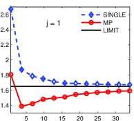
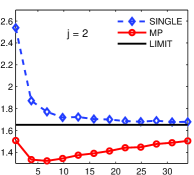
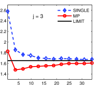
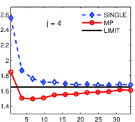
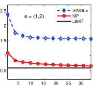
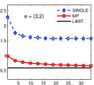
Figure 2: Plots of the slope $\frac{1}{-\log\alpha}\mathbb{E}[\tau_{\mathcal{S}}-\phi|\tau_{\mathcal{S}}\geq\phi]$ against $-\log\alpha$ for message-passing algorithm (MP) and SINGLE algorithm which disregards shared information. The graph is the star graph of $4$ nodes with node $2$ in the center. Estimates of both single and paired change points ($\lambda_{j}$ and $\lambda_{ij}$) are shown together with theoretical limit of Theorem 1. False alarm tolerance $\alpha$ ranges in $[0.5,10^{-13}]$.

We present simulation results as depicted in Fig. 2. The setting is that of graphical model (3) on $d=4$ nodes, where the statistical graph is a star with node $2$ in the middle. Conditioned on $\lambda_{*}$, all the data sequences, $\mathbf{X}_{*}$, are assumed Gaussian of variance $1$, with pre-change mean $1$ and post-change mean zero. All priors are geometric with parameters $\rho_{j}=0.1$. Fig. 2 shows plots of expected delay over $|\log\alpha|$, against $|\log\alpha|$, for two methods: the message-passing algorithm of Section 3.1 (MP) and the method which bases its inference on posteriors calculated based only on each node’s private information (SINGLE). This latter method estimates a single change point $\lambda_{j}$ by $\widehat{\tau}_{j}:=\inf\{n:\,P(\lambda_{j}\leq n|\mathbf{X}_{j}^{n})\geq 1-\alpha\}$ and a paired $\lambda_{ij}=\lambda_{i}\wedge\lambda_{j}$ by $\widehat{\tau}_{i}\wedge\widehat{\tau}_{j}$. Also shown in the figure is the limiting value of the normalized expected delay as predicted by Theorem 1. All plots are generated by Monte Carlo simulation over $5000$ realizations.

In estimating single change points, MP, which takes shared information into account, has a clear advantage over SINGLE, for high to relatively low false alarm values (even, say, around $\alpha\approx e^{-5}$); though, both methods seem to converge to the same slope in the $\alpha\to 0$ limit, as suggested by Theorem 1. (The particular value is $(-\log 0.9+0.5)^{-1}=1.6519$.) Also note that the advantage of MP over SINGLE is more emphasized for node $2$, as expected by its access to shared information from all the three nodes.

For paired change points, the advantage of MP over SINGLE is more emphasized. It is also interesting to note that while MP seems to converge to the expected theoretical limit $(-2\log 0.9+3\cdot 0.5)^{-1}=0.5845$, SINGLE seems to converge to a higher slope (with a reasonable guess being $1.6519$ as in the case of single change points).

In regard to false alarm probability, nonzero values were only observed for the first few values of $\alpha$ considered here, and those were either below or very close to the specified tolerance.

6 Concentration inequalities for marginal likelihood ratios

In this section, we lay the groundwork for the proof of Theorem 1. The main result here is Theorem 2, which establishes concentration inequalities for various terms that appear in an asymptotic expansion of the marginal likelihood ratio, defined in (17) below. These terms (cf. (23) and (24)) are natural by-products of marginalization over a graph and their asymptotic behavior might be of independent interest.

Our standing assumption throughout is that the graph $G=(V,E)$ is complete. This simplifies the arguments without loss of generality, since one can otherwise make the graph complete, by assigning sequences of i.i.d. data to each non-edge (with the same pre- and post- change distributions). These i.i.d. data do not affect the likelihood (as can be verified by examining the representation of Lemma 5) and they do not contribute to asymptotic delay since the corresponding KL informations are zero.

Fix some delay functional $\phi=\tau_{\mathcal{S}}$ throughout this section. We use the following notation regarding conditional probabilities and expectations

$$\mathbb{P}_{\phi}^{k} :=\mathbb{P}(\;\cdot\;\mid\phi=k),\quad\mathbb{E}_{\phi}^{k}:=\mathbb{E}(\;\cdot\;\mid\phi=k)$$

$$\mathbb{P}_{\lambda_{*}}^{m_{*}} :=\mathbb{P}(\;\cdot\;\mid\lambda_{*}=m_{*}),\quad\mathbb{E}_{\lambda_{*}}^{m_{*}}:=\mathbb{E}(\;\cdot\;\mid\lambda_{*}=m_{*}),\;$$

for $k\in\mathbb{N}$ and $m_{*}=(m_{1},\dots,m_{d})\in\mathbb{N}^{d}$. Here $\{\lambda_{*}=m_{*}\}=\cap_{j=1}^{d}\{\lambda_{j}=m_{j}\}$. Furthermore, let

$$\pi_{\phi}^{k}(m_{*}):=\mathbb{P}(\lambda_{*}=m_{*}\mid\phi=k).$$ (16)

Consider the marginal likelihood ratio

$$D_{\phi}^{k,n}:=D_{\phi}^{k}(\mathbf{X}_{*}^{n}):=\frac{P(\mathbf{X}_{*}^{n}\mid\phi=k)}{P(\mathbf{X}_{*}^{n}\mid\phi=\infty)}.$$ (17)

Our asymptotic analysis hinges on the behavior of $\frac{1}{n}\log D_{\phi}^{k}(\mathbf{X}_{*}^{n})$ as $n\to\infty$, under probability measure $\mathbb{P}_{\phi}^{k}$. In particular, as a direct consequences of the results of [18], if one can show that

$$\mathbb{P}_{\phi}^{k}\Big{[}\frac{1}{N}\max_{1\leq n\leq N}\,\log D_{\phi}^{k}(\mathbf{X}_{*}^{k+n})\geq(1+\varepsilon)I_{\phi}\Big{]}\stackrel{{\scriptstyle N\to\infty}}{{\longrightarrow}}0$$ (18)

for all (small) $\varepsilon>0$ and all $k\in\mathbb{N}$, then the “lower bound” follows, $\inf_{\widetilde{\tau}\in\Delta_{\phi}(\alpha)}\mathbb{E}\big{[}\widetilde{\tau}-\phi\mid\widetilde{\tau}\geq\phi\big{]}\geq\frac{|\log\alpha|}{q_{\phi}+I_{\phi}}\big{(}1+o(1)\big{)}$. Furthermore, let

$$T_{\varepsilon}^{k}:=\sup\Big{\{}n\in\mathbb{N}:\;\frac{1}{n}\log D_{\phi}^{k}(\mathbf{X}_{*}^{k+n-1})<I_{\phi}-\varepsilon\Big{\}}.$$

By the results of [18], if one has

$$\mathbb{E}\,T_{\varepsilon}^{\phi}:=\sum_{k=1}^{\infty}\mathbb{P}(\phi=k)\,\mathbb{E}_{\phi}^{k}(T_{\varepsilon}^{k})<\infty,$$ (19)

for all (small) $\varepsilon>0$, then the “upper bound” follows, that is, $\tau_{\mathcal{S}}$ as defined in (9) satisfies $\mathbb{E}[\tau_{\mathcal{S}}-\phi\mid\tau_{\mathcal{S}}\geq\phi]\leq\frac{|\log\alpha|}{q_{\phi}+I_{\phi}}(1+o(1))$.

The following lemma provides sufficient conditions based on concentration inequalities under conditional probability measures $\mathbb{P}_{\lambda_{*}}^{m_{*}}$. In the following $\varepsilon_{0}>0$ is some constant. (See Appendix D for the proof.)

Lemma 4.

Assume that for all $m_{*}\in\mathbb{N}^{d}$ for which $\pi_{\phi}^{k}(m_{*})>0$, one has

$$\mathbb{P}_{\lambda_{*}}^{m_{*}}\Big{\{}\Big{|}\frac{1}{n}\log D_{\phi}^{k}(\mathbf{X}_{*}^{n})-I_{\phi}\Big{|}>\varepsilon\Big{\}}\leq q(n)\exp(-c_{1}n\varepsilon^{2})$$ (20)

for all $n\in\mathbb{N}$ and $\varepsilon\in(0,\varepsilon_{0})$ such that $\sqrt{n}\geq\frac{1}{\varepsilon}p(m_{*},k)$, where $p(\cdot)$ and $q(\cdot)$ are polynomials with constant nonnegative coefficients. Furthermore, assume that both $\pi_{\phi}^{k}(\cdot)$ and $\mathbb{P}(\phi=\cdot)$ have finite polynomial moments. Then both (18) and (19) hold, hence Theorem 1 holds.

Remark 1. The condition of finite polynomial moments for $\pi_{\phi}^{k}(\cdot)$ and $\mathbb{P}(\phi=\cdot)$ is satisfied for a $\phi=\min_{j\in\mathcal{S}}\lambda_{j}$ under geometric priors on $\{\lambda_{j}\}$.

In order to apply Lemma 4 easily, we introduce a notion of “stochastic asymptotic $\varepsilon$-equivalence” for sequence of random variables. To simplify notation, let $\operatorname{supp}(\pi_{\phi}^{k}):=\{m_{*}\in\mathbb{N}^{d}:\;\pi_{\phi}^{k}(m_{*})>0\}$.

Definition 1.

Consider two sequences $\{a_{n}\}$ and $\{b_{n}\}$ of random variables, where $a_{n}=a_{n}(k)$ and $b_{n}=b_{n}(k)$ could depend on a common parameter $k\in\mathbb{N}$. The two sequences are called “asymptotically $\varepsilon$-equivalent” as $n\to\infty$, w.r.t. the collection $\{\mathbb{P}_{\lambda_{*}}^{m_{*}}:\;m_{*}\in\operatorname{supp}(\pi_{\phi}^{k})\}$, and denoted

$$a_{n}\stackrel{{\scriptstyle\varepsilon}}{{\asymp}}b_{n},$$

if there exist polynomials $p(\cdot)$ and $q(\cdot)$ (with constant nonnegative coefficients), and $\varepsilon_{0}>0$, such that for all $m_{*}\in\operatorname{supp}(\pi_{\phi}^{k})$, we have

$$\mathbb{P}_{\lambda_{*}}^{m_{*}}(|a_{n}-b_{n}|\leq\varepsilon)\geq 1-q(n)e^{-c_{1}n\varepsilon^{2}}$$

for all $n\in\mathbb{N}$ and $\varepsilon\in(0,\varepsilon_{0})$ satisfying $\sqrt{n}\varepsilon\geq p(m_{*},k)$. The one-sided version, e.g, $a_{n}\stackrel{{\scriptstyle\varepsilon}}{{\preccurlyeq}}b_{n}$ is defined by replacing $|a_{n}-b_{n}|\leq\varepsilon$ with $a_{n}\leq b_{n}+\varepsilon$. (The constants are independent of $n,m_{*},k$, and $\varepsilon$, but they could depend on other parameters of the problem.)

By application of union bound and algebra, a finite number of asymptotic $\varepsilon$-equivalence statements can be manipulated under some algebraic rules to produce new such statements. Below, we summarize some of the rules:

1. $a_{n}\stackrel{{\scriptstyle\varepsilon}}{{\asymp}}b_{n}$ implies $a_{n}\stackrel{{\scriptstyle C\varepsilon}}{{\asymp}}b_{n}$ for $C>0$ and $\alpha a_{n}\stackrel{{\scriptstyle\varepsilon}}{{\asymp}}\alpha b_{n}$ for $\alpha\in\mathbb{R}$.

2. $a_{n}\stackrel{{\scriptstyle\varepsilon}}{{\asymp}}b_{n}$ and $b_{n}\stackrel{{\scriptstyle\varepsilon}}{{\asymp}}c_{n}$ implies $a_{n}\stackrel{{\scriptstyle\varepsilon}}{{\asymp}}c_{n}$. (Transitivity)

3. $a_{n}\stackrel{{\scriptstyle\varepsilon}}{{\asymp}}b_{n}$ and $c_{n}\stackrel{{\scriptstyle\varepsilon}}{{\asymp}}d_{n}$ implies $a_{n}\pm c_{n}\stackrel{{\scriptstyle\varepsilon}}{{\asymp}}b_{n}\pm d_{n}$.

4. $a_{n}\stackrel{{\scriptstyle\varepsilon}}{{\asymp}}b_{n}$ implies $\max\{a_{n},c_{n}\}\stackrel{{\scriptstyle\varepsilon}}{{\asymp}}\max\{b_{n},c_{n}\}$.

5. $a_{n}\stackrel{{\scriptstyle\varepsilon}}{{\asymp}}b_{n}$, $c_{n}\stackrel{{\scriptstyle\varepsilon}}{{\asymp}}1$ and $\{b_{n}\}$ bounded implies $a_{n}c_{n}\stackrel{{\scriptstyle\varepsilon}}{{\asymp}}b_{n}$.

6. $a_{n}\stackrel{{\scriptstyle\varepsilon}}{{\asymp}}a>0$ and $b_{n}\stackrel{{\scriptstyle\varepsilon}}{{\preccurlyeq}}-b<0$ implies $\max\{a_{n},b_{n}\}\stackrel{{\scriptstyle\varepsilon}}{{\asymp}}a$.

7. “log–sum-max” inequality for positive sequences $\{a_{n}\}$ and $\{b_{n}\}$:

   $$n^{-1}\log(a_{n}+b_{n})\stackrel{{\scriptstyle\varepsilon}}{{\asymp}}\max\{n^{-1}\log a_{n},n^{-1}\log b_{n}\}.$$ (21)

The last statement follows from inequalities $0\leq\log(a_{n}+b_{n})-\max\{\log a_{n},\log b_{n}\}\leq\log 2$. Dividing by $n$, we observe that the difference is bounded by $\varepsilon$, in absolute value, as long as $n\varepsilon\geq\log 2$. This implies the condition in Definition 1, since $\{(n,\varepsilon):\sqrt{n}\varepsilon\geq\log 2\}\subset\{(n,\varepsilon):n\varepsilon\geq\log 2\}$.

As another example of how these rules are obtained, consider (R3). We have $|a_{n}-b_{n}|\leq\varepsilon$ on event $A_{1,n}$ having probability at least $1-q_{1}(n)e^{-c_{1}n\varepsilon^{2}}$, for $\sqrt{n}\varepsilon\geq p_{1}(m_{*},k)$. Similarly, $|b_{n}-c_{n}|\leq\varepsilon$ on event $A_{2,n}$ with probability at least $1-q_{2}(n)e^{-c_{2}n\varepsilon^{2}}$, for $\sqrt{n}\varepsilon\geq p_{2}(m_{*},k)$. Then, by union bound $A_{1,n}\cap A_{2,n}$ has probability at least $1-(q_{1}(n)+q_{2}(n))e^{-(c_{1}\wedge c_{2})n\varepsilon^{2}}$, for $\sqrt{n}\varepsilon\geq p_{1}(m_{*},k)+p_{2}(m_{*},k)$. For this range of $n$, on event $A_{1,n}\cap A_{2,n}$, we have both $|a_{n}-b_{n}|\leq\varepsilon$ and $|b_{n}-c_{n}|\leq\varepsilon$, from which it follows $|a_{n}-c_{n}|\leq 2\varepsilon$, by triangle inequality. Since both $q_{1}+q_{2}$ and $p_{1}+p_{2}$ are polynomials, we have the desired assertion.

Remark 1 According to Definition 1 and Lemma 4, to prove Theorem 1, it is enough to show that

$$\frac{1}{n}\log D_{\phi}^{k,n}\stackrel{{\scriptstyle\varepsilon}}{{\asymp}}I_{\phi}\quad\text{as $n\to\infty$ w.r.t. $\{\mathbb{P}_{\lambda_{*}}^{m_{*}}\}$}$$

(We often omit $m_{*}\in\operatorname{supp}(\pi_{\phi}^{k})$ when it is implicitly understood.) The rules stated above allows one to reduce the problem to asymptotic $\varepsilon$-equivalence statements for simpler terms, as considered in the next section. In this context, we regard parameters of the priors, $\{\rho_{j}\}$, and pre- and post-change densities as constants. In other words, the constants in the definition of $\varepsilon$-equivalence can depend on $\{\rho_{j}\}$, $\{I_{e}\}$, and $M$ (the uniform norm of $\log(f_{e}/g_{e})$).

We now introduce a couple of building blocks occurring frequently and establish $\stackrel{{\scriptstyle\varepsilon}}{{\asymp}}$ statements for them. Recall that $f_{e}$ and $g_{e}$ denote the pre- and post-change densities for edge $e\in\widetilde{E}$. Define

$$R_{k}^{n}(e):=R_{k}^{n}(\mathbf{X}_{e}):=\prod_{t=k}^{n}\frac{f_{e}}{g_{e}}(\mathbf{X}_{e})=\prod_{t=k}^{n}e^{h_{e}(\mathbf{X}_{e})},\quad h_{e}:=\log\frac{f_{e}}{g_{e}}.$$ (22)

Note that by assumption $\|h_{e}\|_{\infty}\leq M$ for all $e$. We will use the convention that empty products evaluate to $1$, that is, $R_{k}^{n}(e)=1$ whenever $k>n$. We also define $S$-terms as

$$S_{u}^{\nu,n}(e):=\sum_{p=u}^{\nu}Ae^{-\beta p}R_{p}^{n}(e)$$ (23)

where $A$ and $\beta$ are some positive constants. Similarly, define $M$ and $L$-terms as follows

$$M_{u}^{\nu,n}(e) :=\sum_{p_{1}=u}^{\nu}\sum_{p_{2}=u}^{\nu}Ae^{-(\beta_{1}p_{1}+\beta_{2}p_{2})}R_{p_{1}\wedge p_{2}}^{n}(e)$$ (24)

$$L_{u,(r)}^{\nu,n}(e) :=\sum_{p=u}^{\nu}Ae^{-\beta p}R_{p\wedge r}^{n}(e)$$ (25)

for constants $A,\beta_{1},\beta_{2},\beta>0$. The constants involved in these definitions can be different in each occurrence and we have suppressed them in the notation for simplicity. The $M$ and $L$-terms are most relevant when $e$ is a proper edge, that is, $e=\{i,j\}\in\widetilde{E}$ and $i\neq j$, although the statements involving them hold in general.

The following lemma is proved in Section 8. Recall that $I_{e}$ is the KL divergence between $f_{e}$ and $g_{e}$, that is, $I_{e}:=\int f_{e}\log\frac{f_{e}}{g_{e}}$.

Theorem 2.

Assume $\|\log\frac{f_{e}}{g_{e}}\|_{\infty}\leq M$ for all $e\in\widetilde{E}$. The following asymptotic $\varepsilon$-equivalence relations hold with respect to $\{\mathbb{P}_{\lambda_{*}}^{m_{*}}:\;m_{*}\in\operatorname{supp}(\pi_{\phi}^{k})\}$, as $n\to\infty$,

$$\frac{1}{n}\log R_{u}^{n}(e)\,\stackrel{{\scriptstyle\varepsilon}}{{\asymp}}\,\frac{1}{n}\log S_{u}^{\infty,n}(e)\,\stackrel{{\scriptstyle\varepsilon}}{{\asymp}}\,\frac{1}{n}\log M_{u}^{\infty,n}(e)\,\stackrel{{\scriptstyle\varepsilon}}{{\asymp}}\,\frac{1}{n}\log L_{u,(r)}^{\infty,n}(e)\,\stackrel{{\scriptstyle\varepsilon}}{{\asymp}}\,I_{e}$$ (26)

for any $u,r\leq 2k$ and $e\in\widetilde{E}$.

The proof of this theorem is deferred to Section 8. The $\log\varepsilon$-equivalence $\frac{1}{n}\log R_{u}^{n}(e)\stackrel{{\scriptstyle\varepsilon}}{{\asymp}}I_{e}$ is intuitive as will become clear in the proof. The lemma essentially states that there are no surprises regarding $S$, $M$ and $L$ terms and they are all $\varepsilon$-equivalent to the corresponding edge information. We also note that $2k$ in the statement of the Lemma can be replaced with $Ck$ for any constant $C>0$.

Remark. Let us consider the role of our assumptions on the priors and likelihood ratios, by giving a high-level overview of the proof of Theorem2 for $S_{u}^{\infty,n}(e)$. The exponential decay for the tails of the priors is reflected in the definition of $S_{u}^{\infty,n}(e)$ in in (23). The terms $R_{p}^{n}(e)$ in this sum are concentrated around $I_{e}$ if $p\ll n$ (as in this case $R_{p}^{n}(e)$ is the product of many essentially i.i.d. terms). For $p$ close to $n$, however, there is no guaranteed concentration for $R_{p}^{n}(e)$, as it is a product of only a few random variables. For these terms, however, the prefactor $e^{-\beta p}$ is small while $R_{p}^{n}(e)$ is gauranteed to be bounded (based on $\|\log(f_{e}/g_{e})\|_{\infty}\leq M$). Hence these terms are a negligible and do not contribute to $\frac{1}{n}\log S_{u}^{\infty,n}(e)$, asymptotically. This argument is made precise in Section 8.

To simplify notation, from now on, we will drop the second upper index in the symbols for $S$, $L$ and $M$ terms, whenever this index is $n$ and there is no chance of confusion. That is, we adhere to the following convention,

$$S_{u}^{\nu}(e):=S_{u}^{\nu,n}(e),\quad L_{u,(r)}^{\nu}(e):=L_{u,(r)}^{\nu,n}(e),\quad M_{u}^{\nu}(e):=M_{u}^{\nu,n}(e).$$ (27)

7 Proof of the optimal delay theorem

Let us define

$$\mathcal{M}_{\phi}^{k,n}:=\mathcal{M}_{\phi}^{k}(\mathbf{X}_{*}^{n}):=\sum_{k_{1},\dots,k_{d}}\pi_{\phi}^{k}(k_{1},\dots,k_{d})\prod_{j\in V}R_{k_{j}}^{n}\{j\}\prod_{e\in E}R_{k_{e}}^{n}(e)$$ (28)

where $k_{e}:=k_{i}\wedge k_{j}$ for $e=\{i,j\}$, and each variable $k_{j}$ runs over $\{1,2,\dots\}\cup\{\infty\}$. The inclusion of $\infty$ in range of the summations does not affect the case $k<\infty$, but will allow us to use the same expression (28) for $\mathcal{M}_{\phi}^{\infty,n}$. We have following easily verified representation of $D_{\phi}^{k,n}$. (See Appendix B for the proof).

Lemma 5.

With $D_{\phi}^{k,n}$ defined as in (17),

$$D_{\phi}^{k,n}=\frac{\mathcal{M}_{\phi}^{k,n}}{\mathcal{M}_{\phi}^{\infty,n}}.$$ (29)

We will use the following technical lemma to decouple sums of products. Let $\binom{[r]}{2}$ denote the collection of 2-subsets of $[r]=\{1,\dots,r\}$, with the convention that each member is a denoted as an ordered pair $(i,j)$ with $i<j$.

Lemma 6.

Let $\bm{S}=S_{1}\times S_{2}\times\cdots\times S_{r}$ be the Cartesian product of $r$ countable sets $S_{1},\dots,S_{r}$ and let $\bm{k}=(k_{1},\dots,k_{r})$ be a multi-index for $\bm{S}$. Let $F_{j}$ and $G_{ij}$ be nonnegative functions defined on $S_{j}$ and $S_{i}\times S_{j}$ respectively, for $i,j\in[r]$. Let $H_{1}$ be a nonnegative function on $S_{1}$. Let $\bm{\beta}=(\beta_{1},\dots,\beta_{r})\in\mathbb{R}_{++}^{r}$. Then,

$$(a) \quad\sum_{k_{1}\in S_{1}}e^{-\beta_{1}k_{1}}F_{1}(k_{1})H_{1}(k_{1})\leq\Big{(}\sum_{k_{1}\in S_{1}}e^{-\beta_{1}k_{1}/2}F_{1}(k_{1})\Big{)}\Big{(}\sum_{k_{1}\in S_{1}}e^{-\beta_{1}k_{1}/2}H_{1}(k_{1})\Big{)}.$$ (30)

$$\begin{split}(b)&\quad\sum_{\bm{k}\,\in\,\bm{S}}\Big{\{}e^{-\bm{\beta}^{T}\bm{k}}\prod_{j=1}^{r}F_{j}(k_{j})\prod_{(i,j)\in\binom{[r]}{2}}G_{ij}(k_{i},k_{j})\Big{\}}\;\leq\;\Big{(}\prod_{j=1}^{r}\Big{\{}\sum_{k_{j}\in S_{j}}e^{-\beta_{j}k_{j}/r}F_{j}(k_{j})\Big{\}}\Big{)}\times\\ &\qquad\qquad\qquad\qquad\qquad\prod_{(i,j)\in\binom{[r]}{2}}\Big{\{}\sum_{(k_{i},k_{j})\in S_{i}\times S_{j}}e^{-(\beta_{i}k_{i}+\beta_{j}k_{j})/r}G_{ij}(k_{i},k_{j})\Big{\}}\end{split}$$ (31)

The key in this lemma is that the functions $F_{j}$, $G_{ij}$ and $H_{1}$ are nonnegative. One might already see how the application of Lemma 6 to the sum in (28) produces $S$ and $M$ terms as introduced in Section 6. We are ready to give the proof of Theorem 1. We start with the two extreme change point functionals $\lambda_{\mathcal{S}}$: a single change point ($|\mathcal{S}|=1$), and the minimum of all the change points ($\mathcal{S}=[d]$). Then, we present the proof for $\lambda_{\mathcal{S}}$ with $1<|\mathcal{S}|<d$, omitting some of the details for brevity.

7.1 Proof for the case $\phi=\lambda_{1}\wedge\cdots\wedge\lambda_{d}$

First, note that in this case $\mathcal{M}_{\phi}^{\infty,n}=1$, since $\phi=\infty$ implies $\lambda_{1}=\cdots=\lambda_{d}=\infty$. Hence, we only need to consider $\mathcal{M}_{\phi}^{k,n}$ for some $k<\infty$. We then observe that $\pi_{\phi}^{k}(k_{1},\dots,k_{d})$ is nonzero only when at least one of $k_{1},\dots,k_{d}$ is equal to $k$. We break up the sum according to how many of $k_{1},\dots,k_{d}$ are equal to $k$.

Let $\mathcal{I}$ be a subset of $[d]$ of size $|\mathcal{I}|=s$. Let $\mathcal{I}^{c}=[d]\setminus\mathcal{I}$. Consider the terms in the sum (28) for which $k_{j}=k$ for $j\in\mathcal{I}$ and $k_{j}>k$ for $j\in\mathcal{I}$. We call the sum over these terms $T_{\mathcal{I}}$. Then, $\mathcal{M}_{\phi}^{k,n}=\sum_{\mathcal{I}:|\mathcal{I}|\geq 1}T_{\mathcal{I}}=\sum_{s=1}^{d}\sum_{\mathcal{I}:|\mathcal{I}|=s}T_{\mathcal{I}}$, where the sum is over all subsets $\mathcal{I}$ of $[d]$ of size at least $1$.

Let us fixed some $s\in[d]$ and some $\mathcal{I}\subset[d]$ with $|\mathcal{I}|=s$. Without loss of generality, we can pick $\mathcal{I}=\{1,\dots,s\}$. We note that

$$\pi_{\phi}^{k}(k,\dots,k,k_{s+1},\dots,k_{d}) =A\prod_{j=s+1}^{d}\overline{\rho}_{j}^{k_{j}}$$

$$=Ae^{-\sum_{j\in\mathcal{I}^{c}}\beta_{j}k_{j}},\quad\text{for}\;k_{j}>k,j\in\mathcal{I}^{c}$$

where $\beta_{j}=-\log\overline{\rho}_{j}>0$, and $A=A(\{\rho_{j}\})$ is some constant. It follows that

$$T_{\mathcal{I}}=\prod_{j\in\,\mathcal{I}}R_{k}^{n}\{j\}\prod_{|e\,\cap\,\mathcal{I}|\,\geq\,1}R_{k}^{n}(e)\underbrace{\sum_{k_{j}>k,\;j\in\mathcal{I}^{c}}\Big{\{}Ae^{-\sum_{j\in\mathcal{I}^{c}}\beta_{j}k_{j}}\prod_{j\in\,\mathcal{I}^{c}}R_{k_{j}}^{n}\{j\}\prod_{|e\,\cap\,\mathcal{I}|=0}R_{k_{e}}^{n}(e)\Big{\}}}_{(\star)}.$$ (32)

Here and in the rest of the proof, the index $e$ runs in the set $E$ of original edges (not the modified set $\widetilde{E}$ introduced in Section 4). That is, each edge $e=\{i,j\}\in E$ for some $i\neq j$. Note that in (32), the rightmost product is over all $2$-subset of $\mathcal{I}^{c}$, which we denote as $\binom{\mathcal{I}^{c}}{2}$. We can now apply first part of Lemma 6, with $r=|\mathcal{I}^{c}|=d-s$, to obtain

$$(\star)\leq A\prod_{j\in\mathcal{I}^{c}}\Big{\{}\underbrace{\sum_{k_{j}>k}e^{-\frac{\beta_{j}k_{j}}{d-s}}R_{k_{j}}^{n}\{j\}}_{(\star\star)}\Big{\}}\prod_{(i,j)\in\binom{\mathcal{I}^{c}}{2}}\Big{\{}\underbrace{\sum_{\begin{subarray}{c}k_{i}>k,\\ k_{j}>k\end{subarray}}e^{-\frac{\beta_{i}k_{i}+\beta_{j}k_{j}}{d-s}}R_{k_{i}\wedge k_{j}}^{n}\{i,j\}}_{(\star\star\star)}\Big{\}}.$$

Each term denoted as $(\star\star)$ is of the form $S_{k+1}^{\infty}\{j\}$ and each term denoted as $(\star\!\star\!\star)$ is of the form $M_{k+1}^{\infty}\{i,j\}$. Hence, we have

$$T_{\mathcal{I}}\;\leq A\prod_{j\in\,\mathcal{I}}R_{k}^{n}\{j\}\prod_{|e\,\cap\,\mathcal{I}|\,\geq\,1}R_{k}^{n}(e)\prod_{j\in\mathcal{I}^{c}}S_{k+1}^{\infty}\{j\}\prod_{|e\,\cap\,\mathcal{I}|=0}M_{k+1}^{\infty}(e).$$

Applying Theorem 2 to each of the $R,S$ and $M$ forms above, we obtain

$$\frac{1}{n}\log T_{\mathcal{I}} \stackrel{{\scriptstyle\varepsilon}}{{\preccurlyeq}}\sum_{j\in\mathcal{I}}I_{j}+\sum_{|e\cap\mathcal{I}|\geq 1}I_{e}+\sum_{j\in\mathcal{I}^{c}}I_{j}+\sum_{|e\,\cap\,\mathcal{I}|=0}I_{e}$$

$$=\sum_{j\,\in\,V}I_{j}+\sum_{e\,\in\,E}I_{e}.$$ (33)

where the $\varepsilon$-equivalence in the above an in what follows is w.r.t. $\{\mathbb{P}_{\lambda_{*}}^{m_{*}}\}$.

To obtain the lower bound, we bound $(\star)$ from below by its first term,

$$(\star)\geq Ae^{-(k+1)\sum_{j\in\mathcal{I}^{c}}\beta_{j}}\prod_{j\,\in\,\mathcal{I}^{c}}R_{k+1}^{n}\{j\}\prod_{|e\,\cap\,\mathcal{I}|=0}R_{k+1}^{n}(e)$$

which, after applying Theorem 2, gives us a lower bound on $\frac{1}{n}\log T_{\mathcal{I}}$ matching the RHS of (33). Finally, note that the RHS of (33) does not depend on the particular choice of $\mathcal{I}$. We now use the log-sum-max rule (R7) to get

$$\frac{1}{n}\log\mathcal{M}_{\phi}^{k,n} =\frac{1}{n}\log\Big{(}\sum_{\mathcal{I}:|\mathcal{I}|\geq 1}T_{\mathcal{I}}\Big{)}$$

$$\stackrel{{\scriptstyle\varepsilon}}{{\asymp}}\max_{\mathcal{I}:|\mathcal{I}|\geq 1}\Big{\{}\frac{1}{n}\log T_{\mathcal{I}}\Big{\}}\stackrel{{\scriptstyle\varepsilon}}{{\asymp}}\sum_{j\,\in\,V}I_{j}+\sum_{e\,\in\,E}I_{e},$$

which is the desired result.

7.2 Proof for the case $\phi=\lambda_{1}$

In this case, one has $\pi_{\phi}^{k}(k_{1},\dots,k_{d})=1\{k_{1}=k\}\prod_{j=2}^{d}\pi_{j}(k_{j})$, hence

$$\pi_{\phi}^{k}(k_{1},\dots,k_{d})=\Big{[}1\{k_{1}=k\}A\prod_{j=2}^{d}\overline{\rho}_{j}^{k_{j}}\Big{]}=\Big{[}1\{k_{1}=k\}Ae^{-\sum_{j=2}^{d}\beta_{j}k_{j}}\Big{]}$$

where $\beta_{j}=-\log\overline{\rho}_{j}>0$ and $A=A(\{\rho_{j}\})>0$ is some constant. Then, we can write

$$\mathcal{M}_{\phi}^{k,n}=R_{k}^{n}\{1\}\sum_{k_{2},\dots,k_{d}}\Big{\{}Ae^{-\sum_{j=2}^{d}\beta_{j}k_{j}}\prod_{j=2}^{d}\Big{(}R_{k_{j}}^{n}\{j\}R_{k\wedge k_{j}}^{n}\{1,j\}\Big{)}\,\prod_{e:\;1\notin e}R_{k_{e}}^{n}(e)\Big{\}}.$$ (34)

Note that the second product runs over all $2$-subsets of $[2:d]:=\{2,\dots,d\}$ which we denote as $\binom{[2:d]}{2}$. Hence, we can apply Lemma 6 with $r=d-1$ to obtain

$$\frac{\mathcal{M}_{\phi}^{k,n}}{AR_{k}^{n}\{1\}}\leq\prod_{j=2}^{d}\Big{\{}\sum_{k_{j}}e^{-\beta_{j}k_{j}/(d-1)}R_{k_{j}}^{n}\{j\}R_{k\wedge k_{j}}^{n}\{1,j\}\Big{\}}\prod_{(i,j)\in\binom{[2:d]}{2}}\Big{\{}\sum_{k_{i},k_{j}}e^{-(\beta_{i}k_{i}+\beta_{j}k_{j})/(d-1)}R_{k_{i}\wedge k_{j}}^{n}\{i,j\}\Big{\}}.$$

Each term appearing in second product is of the form $M_{1}^{\infty}\{i,j\}$. Applying the second half of Lemma 6 to the first product, we get

$$\frac{\mathcal{M}_{\phi}^{k,n}}{AR_{k}^{n}\{1\}}\leq\prod_{j=2}^{d}\Big{\{}\underbrace{\Big{(}\sum_{k_{j}}e^{-\frac{\beta_{j}k_{j}}{2(d-1)}}R_{k_{j}}^{n}\{j\}\Big{)}}_{(*)}\underbrace{\Big{(}\sum_{k_{j}}e^{-\frac{\beta_{j}k_{j}}{2(d-1)}}R_{k\wedge k_{j}}^{n}\{1,j\}\Big{)}}_{(**)}\Big{\}}\prod_{(i,j)\in\binom{[2:d]}{2}}M_{1}^{\infty}\{i,j\}$$ (35)

Each term denoted as $(*)$ is of the form $S_{1}^{\infty}\{j\}$. For $k<\infty$, each term denoted as $(**)$ can be written in the form $L_{1,(k)}^{\infty}\{1,j\}$ . That is,

$$\frac{\mathcal{M}_{\phi}^{k,n}}{AR_{k}^{n}\{1\}}\leq\prod_{j=2}^{d}\Big{\{}S_{1}^{\infty}\{j\}L_{1,(k)}^{\infty}\{1,j\}\Big{\}}\prod_{(i,j)\in\binom{[2:d]}{2}}M_{1}^{\infty}\{i,j\}$$

Applying Theorem 2 to each of the $R$, $S$, $L$ and $M$ forms above, we obtain

$$\frac{1}{n}\log\mathcal{M}_{\phi}^{k,n}\stackrel{{\scriptstyle\varepsilon}}{{\preccurlyeq}}I_{1}+\sum_{j=2}^{d}(I_{j}+I_{1,j})+\sum_{(i,j)\in\binom{[2:d]}{2}}I_{ij}$$ (36)

where the $\varepsilon$-equivalence in the above an in what follows is w.r.t. $\{\mathbb{P}_{\lambda_{*}}^{m_{*}}\}$.

The lower bound is obtained, as in Section 7.1, by bounding the sum in (34) by its first term (i.e., $k_{1}=k_{2}=\cdots=k_{d}=1$)

$$\mathcal{M}_{\phi}^{k,n}\geq R_{k}^{n}\{1\}Ae^{-\sum_{j=2}^{d}\beta_{j}}\prod_{j=2}^{d}R_{1}^{n}\{j\}R_{1}^{n}\{1,j\}\prod_{(i,j)\in\binom{[2:d]}{2}}R_{1}^{n}\{i,j\}.$$

Applying $\frac{1}{n}\log(\cdot)$ and using Theorem 2 for each term, we get a lower bound matching the RHS of (36). That is, the bound in (36) holds with $\stackrel{{\scriptstyle\varepsilon}}{{\preccurlyeq}}$ replaced with $\stackrel{{\scriptstyle\varepsilon}}{{\asymp}}$.

Now consider the denominator of $D_{\phi}^{k,n}$, namely $\mathcal{M}_{\phi}^{\infty,n}$. An upper bound on $\mathcal{M}_{\phi}^{\infty,n}$ can be obtained by letting $k=\infty$ in (35). We note that $R_{\infty}^{n}\{1\}=1$ and that $(**)$ is now a term of the form $S_{1}^{\infty}\{1,j\}$. Proceeding as before, we obtain an upper bound similar to that of (36), with $I_{1}$ missing from the bound. The lower bound is obtained by the same technique. Hence,

$$\frac{1}{n}\log\mathcal{M}_{\phi}^{\infty,n}\;\stackrel{{\scriptstyle\varepsilon}}{{\asymp}}\;\sum_{j=2}^{d}(I_{j}+I_{1,j})+\sum_{(i,j)\in\binom{[2:d]}{2}}I_{ij}.$$ (37)

Combining equality form of (36) and (37), we have

$$\frac{1}{n}\log D_{\phi}^{k,n}=\frac{1}{n}\log\mathcal{M}_{\phi}^{k,n}-\frac{1}{n}\log\mathcal{M}_{\phi}^{\infty,n}\;\stackrel{{\scriptstyle\varepsilon}}{{\asymp}}\;I_{1}$$ (38)

which is the desired result.

7.3 Proof for $\lambda_{\mathcal{S}}$ with $1<|\mathcal{S}|<d$

We now briefly give the proof for the remaining cases. Without loss of generality, we assume $\mathcal{S}=\{1,2,\dots,r\}$ for some $r\in\{2,\dots,d-1\}$. In other words, the delay functional is $\phi=\lambda_{\mathcal{S}}=\lambda_{1}\wedge\lambda_{2}\wedge\cdots\wedge\lambda_{r}$. We observe that $\pi_{\phi}^{k}(k_{1},\dots,k_{d})$ is nonzero when all of $k_{1},\dots,k_{r}$ are $\geq k$, while at least one of them is equal to $k$. Consider $\mathcal{M}_{\phi}^{k,n}$ for $k<\infty$. As in Section 7.1, we break up the sum in its definition according to how many of $k_{1},\dots,k_{d}$ are equal to $k$.

Let $\mathcal{I}$ be a subset of $\mathcal{S}=[r]$ of size $|\mathcal{I}|=s\leq r$. Let $\mathcal{L}:=\mathcal{S}\setminus\mathcal{I}$ and $\mathcal{S}^{c}:=[d]\setminus\mathcal{S}$. Note that $\{\mathcal{I},\mathcal{L},\mathcal{S}^{c}\}$ form a partition of the index set $[d]$. To simplify notation, let $\mathcal{I}^{c}=[d]\setminus\mathcal{I}$ and note that $\mathcal{I}^{c}=\mathcal{L}\cup\mathcal{S}^{c}$.

Consider the terms in the sum (28) for which $k_{j}=k$ for $j\in\mathcal{I}$ and $k_{j}>k$ for $j\in\mathcal{L}$. We call the sum over these terms $T_{\mathcal{I}}$. Then, $\mathcal{M}_{\phi}^{k,n}=\sum_{s=1}^{r}\sum_{\mathcal{I}:|\mathcal{I}|=s}T_{\mathcal{I}}$.

Now fix some $s\in[r]$ and some $\mathcal{I}\subset\mathcal{S}$ with $|\mathcal{I}|=s$. The $R$-terms in the expression of $T_{\mathcal{I}}$ corresponding to nodes are easy to deal with. For the $R$-terms corresponding to edges, we first break them into three categories, based on how many of the endpoints are in $\mathcal{I}$ (i.e., $|e\cap\mathcal{I}|=0,1,2$). The case where exactly one endpoint is in $\mathcal{I}$ (i.e., $|e\cap\mathcal{I}|=1$) is further broken into two cases based on whether the other endpoint is in $\mathcal{L}$ or in $\mathcal{S}^{c}$. The former case, i.e. $|e\cap\mathcal{I}|=|e\cap\mathcal{L}|=1$ behaves the same as the case $|e\cap\mathcal{I}|=2$. We thus combine these two cases, denoted as $|e\cap\mathcal{I}|\geq 1,e\subset\mathcal{S}$. To summarize, we break the edges into a total of three categories. We get the following decomposition

$$T_{\mathcal{I}}=\prod_{j\in\,\mathcal{I}}R_{k}^{n}\{j\}\!\prod_{\begin{subarray}{c}|e\,\cap\,\mathcal{I}|\,\geq\,1,\\ e\,\subset\,\mathcal{S}\end{subarray}}R_{k}^{n}(e)\;\times\\ \sum_{\begin{subarray}{c}k_{j}\,>\,k,\;j\in\mathcal{L}\\ k_{j}\,\geq\,1,\;j\in\mathcal{S}^{c}\end{subarray}}\Big{\{}Ae^{-\sum_{j\in\mathcal{I}^{c}}\beta_{j}k_{j}}\underbrace{\prod_{j\in\,\mathcal{I}^{c}}R_{k_{j}}^{n}\{j\}}_{(*)}\underbrace{\prod_{\begin{subarray}{c}|e\,\cap\,\mathcal{I}|=1,\\ e\,\cap\,\mathcal{S}^{c}=\{\ell\}\end{subarray}}R_{k\wedge k_{\ell}}^{n}(e)}_{(**)}\underbrace{\prod_{|e\,\cap\,\mathcal{I}|=0}R_{k_{e}}^{n}(e)}_{(***)}\Big{\}}$$ (39)

As in Sections 7.1 and 7.2, we can apply Lemma 6 to decouple the sum and obtain an upper bound on $T_{\mathcal{I}}$. The products denoted by $(*)$, $(**)$ and $(*\!*\!*)$ produce $S$, $L$, and $M$-terms, respectively. Using the same lower bounding technique and applying Theorem 2, we obtain

$$\frac{1}{n}\log T_{\mathcal{I}} \stackrel{{\scriptstyle\varepsilon}}{{\asymp}}\sum_{j\,\in\,\mathcal{I}}I_{j}+\sum_{\begin{subarray}{c}|e\,\cap\,\mathcal{I}|\,\geq\,1,\\ e\,\subset\,\mathcal{S}\end{subarray}}I_{e}+\sum_{j\,\in\,\mathcal{I}^{c}}I_{j}+\sum_{\begin{subarray}{c}|e\,\cap\,\mathcal{I}|=1,\\ |e\,\cap\,\mathcal{S}^{c}|=1\end{subarray}}I_{e}+\sum_{|e\,\cap\,\mathcal{I}|=0}I_{e}$$

$$=\sum_{j\in V}I_{j}+\sum_{e\in E}I_{e}.$$

Since this expression does not depend on $\mathcal{I}$, using log-sum-max rule (R7) as before, we obtain that $\frac{1}{n}\log\mathcal{M}_{\phi}^{k,n}\stackrel{{\scriptstyle\varepsilon}}{{\asymp}}\sum_{j\in V}I_{j}+\sum_{e\in E}I_{e}$.

Now, we need to analyze $\mathcal{M}_{\phi}^{\infty,n}$. We try to break up the sum as before into $\widetilde{T}_{\mathcal{I}}$ terms (defined similar to $T_{\mathcal{I}}$ for $\mathcal{M}_{\phi}^{k,n}$). This time however, we only need to consider $\mathcal{I}=\mathcal{S}$ (and $\mathcal{L}$ the empty set), because $\phi=\infty$ implies $\lambda_{j}=\infty$ for all $j\in\mathcal{S}$. The expansion for $\widetilde{T}_{\mathcal{S}}$ can be obtained from (39) by setting $k=\infty$ and removing the terms corresponding to indices in $\mathcal{S}=\mathcal{I}\cup\mathcal{L}$,

$$\mathcal{M}_{\phi}^{\infty,n}=\widetilde{T}_{\mathcal{S}}=\sum_{k_{j}\,\geq\,1,\;j\in\mathcal{S}^{c}}\Big{\{}Ae^{-\sum_{j\in\mathcal{S}^{c}}\beta_{j}k_{j}}\prod_{j\in\mathcal{S}^{c}}R_{k_{j}}^{n}\{j\}\prod_{\begin{subarray}{c}|e\,\cap\,\mathcal{S}|=1,\\ e\,\cap\,\mathcal{S}^{c}=\{\ell\}\end{subarray}}R_{k_{\ell}}^{n}(e)\prod_{|e\,\cap\,\mathcal{S}|=0}R_{k_{e}}^{n}(e)\Big{\}}.$$

It follows that

$$\frac{1}{n}\log\mathcal{M}_{\phi}^{\infty,n}\stackrel{{\scriptstyle\varepsilon}}{{\asymp}}\;\sum_{j\in\mathcal{S}^{c}}I_{j}+\sum_{\begin{subarray}{c}|e\,\cap\,\mathcal{S}|=1,\\ |e\,\cap\,\mathcal{S}^{c}|=1\end{subarray}}I_{e}+\sum_{|e\,\cap\,\mathcal{S}|=0}I_{e}.$$

The last two sums can be described as the sum over all edges $e:e\cap\mathcal{S}^{c}\neq\emptyset$. Putting the pieces together, we have

$$\frac{1}{n}\log D_{\phi}^{k,n} \stackrel{{\scriptstyle\varepsilon}}{{\asymp}}\Big{(}\sum_{j\in V}I_{j}+\sum_{e\in E}I_{e}\Big{)}-\Big{(}\sum_{j\in\mathcal{S}^{c}}I_{j}+\sum_{e\,\cap\,\mathcal{S}^{c}\neq\emptyset}I_{e}\Big{)}$$

$$=\sum_{j\in\mathcal{S}}I_{j}+\sum_{e\,\subset\,\mathcal{S}}I_{e}$$

as desired.

8 Proof of Theorem 2

Let us start by understanding the asymptotic behavior of $\frac{1}{n}\log R_{u}^{n}(e)$. Throughout, we fix $e\in\widetilde{E}$. We either have $e=\{j\}$ in which case $\lambda_{e}=\lambda_{j}$, or $e=\{i,j\}$ in which case $\lambda_{e}=\lambda_{i}\wedge\lambda_{j}$. Recall that $m_{*}=(m_{1},\dots,m_{d})\in\mathbb{N}^{d}$ is a multi-index, and we will work under the collection $\{\mathbb{P}_{\lambda_{*}}^{m_{*}}\}$ of conditional distributions (see Definition 1 for details). The same convention is used regarding the meaning of $m_{e}$, that is, $m_{e}=m_{j}$ for $e=j$, and $m_{e}=m_{i}\wedge m_{j}$ for $e=\{i,j\}$. We also fix some $k\in\mathbb{N}$, which is the parameter $k$ appearing in Definition 1 (reserved for the ultimate conditioning on $\{\phi=k\}$). Finally, we always assume $\varepsilon\in(0,1)$.

At first, we need to be careful about whether $u<m_{e}$ or $u\geq m_{e}$.

Lemma 7.

Let $u\in[n]$ and assume $u\geq m_{e}$. Then,

$$\mathbb{P}_{\lambda_{*}}^{m_{*}}\Big{(}\Big{|}\frac{1}{n-u+1}\log R_{u}^{n}(e)-I_{e}\Big{|}>\varepsilon\Big{)}\leq 2\exp\Big{[}{-\frac{(n-u+1)\varepsilon^{2}}{2M^{2}}}\Big{]}$$ (40)

Proof.

Since $m_{e}\leq u$, conditioned on $\mathbb{P}_{\lambda_{*}}^{m_{*}}$, $\mathbf{X}_{e}^{u},\mathbf{X}_{e}^{u+1},\dots$ are i.i.d. from $f_{e}$. Recalling definition (22), $\log R_{u}^{n}(e)=\sum_{t=u}^{n}h_{e}(\mathbf{X}_{e}^{t})$ which is a sum of $(n-u+1)$ i.i.d. bounded variables $h_{e}(\mathbf{X}_{e}^{t})\in[-M,M]$ with mean $\mathbb{E}_{f_{e}}h_{e}(\mathbf{X}_{e}^{u})=I_{e}$. The result then follows from Hoeffding inequality. ∎

Before moving on, we need an extension of Definition 1. We need to deal with intermediate sequences whose terms depend possibly on $m_{*}$ (in addition to $k$). There is nothing to preclude such dependence in Definition 1. Hence, we use the same definition for $\varepsilon$-equivalence of such sequences with respect to the collection $\{\mathbb{P}_{\lambda_{*}}^{m_{*}}\}$. Note that for any $u,\nu\in\mathbb{N}$, we can write

$$R_{u}^{n}(e)=R_{u}^{\nu-1}(e)R_{u\vee\nu}^{n}(e)$$ (41)

which holds irrespective of whether $u\geq\nu$ or $u<\nu$.

Lemma 8.

For any $u\in[k]$, $\frac{1}{n}\log R_{u\vee m_{e}}^{n}(e)\stackrel{{\scriptstyle\varepsilon}}{{\asymp}}I_{e}$ as $n\to\infty$ with respect to $\{\mathbb{P}_{\lambda_{*}}^{m_{*}}\}$

Lemma 9.

For any $u\in\mathbb{N}$, $\frac{1}{n}\log R_{u}^{m_{e}-1}(e)\stackrel{{\scriptstyle\varepsilon}}{{\asymp}}0$ as $n\to\infty$ with respect to $\{\mathbb{P}_{\lambda_{*}}^{m_{*}}\}$.

Lemma 10.

For any $u\in[k]$, $\frac{1}{n}\log R_{u}^{n}(e)\stackrel{{\scriptstyle\varepsilon}}{{\asymp}}I_{e}$ as $n\to\infty$ with respect to $\{\mathbb{P}_{\lambda_{*}}^{m_{*}}\}$.

The last lemma proves the statement in Theorem 2 regarding asymptotic behavior of $\frac{1}{n}\log R_{u}^{n}(e)$ for $u\in[k]$.

Proof of Lemma 8.

Apply Lemma 7 with $u$ replaced with $u\vee m_{e}$. Since $\varepsilon<1$ and $u\vee m_{e}\leq k\vee m_{e}$, the RHS of (40) is further bounded above by

$$2\exp\Big{(}\frac{(k\vee m_{e})\varepsilon}{2M^{2}}\Big{)}\exp\Big{(}{-\frac{n\varepsilon^{2}}{2M^{2}}}\Big{)}\leq 2\exp\Big{(}{-\frac{n\varepsilon^{2}}{4M^{2}}}\Big{)}$$

as long as $(k\vee m_{e})\varepsilon\leq n\varepsilon^{2}/2$ or equivalently $n\varepsilon\geq 2(k\vee m_{e})$. (This same condition guarantees $u\vee m_{e}\in[n]$ justifying application of Lemma 7.) The condition obtained is of the form required by Definition 1, since $2(k\vee m_{e})$ is bounded above by a polynomial, say $2(k+m_{i})$ if $e=\{i,j\}$. This shows that

$$\frac{1}{n-u\vee m_{e}+1}\log R_{u\vee m_{e}}^{n}(e)\stackrel{{\scriptstyle\varepsilon}}{{\asymp}}I_{e}\quad\text{ w.r.t.}\;\{\mathbb{P}_{\lambda_{*}}^{m_{*}}\}.$$

Now, note that $|\frac{n-u\vee m_{e}+1}{n}-1|\leq\frac{u\vee m_{e}-1}{n}\leq\frac{k\vee m_{e}}{n}$ which can be made $\leq\varepsilon$ by choosing $n\varepsilon\geq(k\vee m_{e})$. This implies that $\frac{n-u\vee m_{e}+1}{n}\stackrel{{\scriptstyle\varepsilon}}{{\asymp}}1$. Applying rule (R5), with $a_{n}=\frac{1}{n-u\vee m_{e}+1}\log R_{u\vee m_{e}}^{n}(e)$, $b_{n}=I_{e}$ and $c_{n}=\frac{n-u\vee m_{e}+1}{n}$, we obtain the desired result. ∎

Proof of Lemma 9.

If $u>m_{e}-1$, we have by definition $R_{u}^{m_{e}-1}(e)=1$ and there is nothing to show. Otherwise, by boundedness assumption $\|h\|_{\infty}\leq M$, we have

$$e^{-Mm_{e}}\leq e^{-M(m_{e}-u)}\leq R_{u}^{m_{e}-1}(e)\leq e^{M(m_{e}-u)}\leq e^{Mm_{e}}.$$

Hence, by taking $n\varepsilon\geq Mm_{e}$, we have $|\frac{1}{n}\log R_{u}^{m_{e}-1}(e)|\leq\varepsilon$, which implies the result. ∎

Proof of Lemma 10.

Apply (41) with $\nu=m_{e}$, to obtain

$$\frac{1}{n}\log R_{u}^{n}(e)=\frac{1}{n}\log R_{u}^{m_{e}-1}(e)+\frac{1}{n}\log R_{u\vee m_{e}}^{n}(e).$$

The result now follows from Lemmas 8 and 9 and rule (R3). ∎

8.1 Bounding $S$-terms

Bounding $S$-terms is perhaps the most elaborate part of the proof. We start with a uniformization of Lemma 7 and then proceed in steps, working on various parts of the sum $S_{u}^{\infty}(e):=S_{u}^{\infty,n}(e)$ one at a time. Up to Lemma 16, we will use the shorthand notation introduced in (27), with $n$ superscript dropped. It might help to recall that in this notation, $u$ and $\infty$ are the initial and final indices of the sum, respectively. Also, the edge $e\in E$ is fixed throughout.

Lemma 11.

Let $u\in\mathbb{N}$ and $\alpha\in(0,1)$ such that $m_{e}\leq u\leq\lfloor\alpha n\rfloor$. Then,

$$\sup_{u\,\leq\,p\,\leq\,\lfloor\alpha n\rfloor}\Big{|}\frac{1}{n-p+1}\log R_{p}^{n}(e)-I_{e}\Big{|}\leq\varepsilon$$

with $\mathbb{P}_{\lambda_{*}}^{m_{*}}$-probability at least $1-2(\lfloor\alpha n\rfloor-u+1)\exp[-\frac{\varepsilon^{2}((1-\alpha)n+1)}{2M^{2}}]$.

Lemma 12.

Let $u\in[k]$ and $\alpha\in(0,1)$ such that $m_{e}\leq u\leq\lfloor\alpha n\rfloor$. Then

$$\mathbb{P}_{\lambda_{*}}^{m_{*}}\Big{(}\Big{|}\frac{1}{n}\log S_{u}^{\lfloor\alpha n\rfloor}(e)-I_{e}\Big{|}\leq 2\varepsilon\Big{)}\geq 1-2n\exp\Big{(}{-\frac{1-\alpha}{2M^{2}}n\varepsilon^{2}}\Big{)}$$

for $n\varepsilon\geq c_{0}k$ and $\varepsilon\in(0,1)$.

Lemma 13.

Let $\delta\in(0,1)$ and $\alpha=\frac{M+\delta\beta}{M+\beta}$. Then, for $n\geq n_{0}(A,\beta,M,\delta)$,

$$\frac{1}{n}\log S_{\lfloor\alpha n\rfloor+1}^{n}(e)\leq-\frac{\delta}{2}\beta.$$

Lemma 14.

Let $\alpha=\frac{M+\frac{1}{2}\beta}{M+\beta}$ and $u\in[k]$. Then, $\frac{1}{n}\log S_{u\vee m_{e}}^{\lfloor\alpha n\rfloor}(e)\stackrel{{\scriptstyle\varepsilon}}{{\asymp}}I_{e}$ as $n\to\infty$ w.r.t. $\{\mathbb{P}_{\lambda_{*}}^{m_{*}}\}$.

Lemma 15.

For any $u\in[k]$, we have $\frac{1}{n}\log S_{u\vee m_{e}}^{n}(e)\stackrel{{\scriptstyle\varepsilon}}{{\asymp}}I_{e}$ as $n\to\infty$ w.r.t. $\{\mathbb{P}_{\lambda_{*}}^{m_{*}}\}$.

Proof of Lemma 11.

We note that for any $p=u,u+1,\dots,\lfloor\alpha n\rfloor$, Lemma 7 applies. We can further upper-bound the RHS of (40) by

$$2\exp\Big{[}{-\frac{(n-p+1)\varepsilon^{2}}{2M^{2}}}\Big{]}\leq 2\exp\Big{[}{-\frac{(n-\alpha n+1)\varepsilon^{2}}{2M^{2}}}\Big{]}.$$

The result follows by applying union bound. ∎

Proof of Lemma 12.

By Lemma 11, uniformly over $p=u,\dots,\lfloor\alpha n\rfloor$, we have

$$e^{(n-p+1)(I_{e}-\varepsilon)}\leq R_{p}^{n}(e)\leq e^{(n-p+1)(I_{e}+\varepsilon)}$$ (42)

with $\mathbb{P}_{\lambda_{*}}^{m_{*}}$-probability at least $1-2n\exp(-\frac{(1-\alpha)n\varepsilon^{2}}{2M^{2}})$. (Note that this is a further lower bound w.r.t. that of Lemma 11) On the event that (42) holds, we have

$$S_{u}^{\lfloor\alpha n\rfloor}(e) \leq\sum_{p=u}^{\lfloor\alpha n\rfloor}Ae^{-\beta p}e^{(n-p+1)(I_{e}+\varepsilon)}$$

$$\leq Ae^{(n+1)(I_{e}+\varepsilon)}\sum_{p=1}^{\infty}e^{-(\beta+I_{e})p}=\frac{Ae^{(n+1)(I_{e}+\varepsilon)}}{e^{\beta+I_{e}}-1}.$$

Take $C_{1}:=\max\{0,\log\frac{A}{e^{\beta+I_{e}}-1}\}$. Then,

$$\frac{1}{n}\log S_{u}^{\lfloor\alpha n\rfloor}(e)\leq\frac{C_{1}}{n}+\frac{n+1}{n}(I_{e}+\varepsilon)\leq I_{e}+2\varepsilon$$

as long as $n\varepsilon\geq C_{1}+I_{e}+1$ (and $\varepsilon<1$). To get the lower bound, we note that (42) implies

$$S_{u}^{\lfloor\alpha n\rfloor}(e) \geq\sum_{p=u}^{\lfloor\alpha n\rfloor}Ae^{-\beta p}e^{(n-p+1)(I_{e}-\varepsilon)}$$

$$\geq Ae^{(n+1)(I_{e}-\varepsilon)}e^{-(\beta+I_{e})u}$$

where we have lower bounded a sum of nonnegative terms by its first term. Hence,

$$\frac{1}{n}\log S_{u}^{\lfloor\alpha n\rfloor}(e)\geq\frac{n+1}{n}(I_{e}-\varepsilon)-\frac{|\log A|+(\beta+I_{e})u}{n}$$

$$\geq I_{e}-\varepsilon-\frac{1+|\log A|+(\beta+I_{e})k}{n}\geq I_{e}-2\varepsilon$$

as long as $n\varepsilon\geq 1+|\log A|+(\beta+I_{e})k$. ∎

Proof of Lemma 13.

By boundedness assumption $\|h\|_{\infty}\leq M$, we have $R_{p}^{n}(e)\leq e^{(n-p+1)M}$ as long as $p\leq n$. Hence,

$$S_{\lfloor\alpha n\rfloor+1}^{n}(e) \leq\sum_{p=\lfloor\alpha n\rfloor+1}^{n}Ae^{-\beta p}e^{(n-p+1)M}$$

$$=Ae^{(n+1)M}\sum_{p=\lfloor\alpha n\rfloor+1}^{n}e^{-(\beta+M)p}$$

$$\leq Ae^{(n+1)M}(n-\alpha n+1)e^{-(\beta+M)\alpha n}$$

where we have used $\lfloor\alpha n\rfloor>\alpha n-1$. Taking $\alpha$ to be as stated and noting that $1-\alpha\in(0,1)$, we get

$$\frac{1}{n}S_{\lfloor\alpha n\rfloor+1}^{n}(e)\leq\frac{|\log A|}{n}+\frac{n+1}{n}M+\frac{\log((1-\alpha)n+1)}{n}-M-\delta\beta\leq-\frac{\delta}{2}\beta$$

as long as $n\geq n_{0}(A,\beta,M,\delta)$ for some $n_{0}$ large enough. ∎

Proof of Lemma 14.

Apply Lemma 12 with $u$ replaced with $u\vee m_{e}$. To ensure $u\vee m_{e}\leq\lfloor\alpha n\rfloor$, let $n\geq\frac{1}{\alpha}(k\vee m_{e}+1)$. To ensure that the bound of Lemma 12 holds, let $n\varepsilon\geq c_{0}k$. Since, these two conditions are met if $n\varepsilon\geq\frac{1}{\alpha}(k+m_{e})+c_{0}k$, the result follows. (Note also that $\frac{1-\alpha}{2M^{2}}$ is a positive constant by our choice of $\alpha$.) ∎

Proof of Lemma 15.

Let $\alpha=\frac{M+\frac{1}{2}\beta}{M+\beta}$ and as in Lemma 14 assume $n\geq\frac{1}{\alpha}(k\vee m_{e}+1)$ so that $u\vee m_{e}\leq\lfloor\alpha n\rfloor$. (This is just to make sure that sums ranging from $u\vee m_{e}$ to $\lfloor\alpha n\rfloor$ are not vacuous.) By Lemma 12, we have

$$\frac{1}{n}\log S_{\lfloor\alpha n\rfloor+1}^{n}(e)\stackrel{{\scriptstyle\varepsilon}}{{\preccurlyeq}}-\frac{1}{4}\beta$$

and by Lemma 14, $\frac{1}{n}\log S_{u\vee m_{e}}^{\lfloor\alpha n\rfloor}(e)\stackrel{{\scriptstyle\varepsilon}}{{\asymp}}I_{e}$. Now, we can break up the sum and use log-sum-max rule (R7),

$$\frac{1}{n}\log S_{u\vee m_{e}}^{n}(e) =\frac{1}{n}\log\Big{(}S_{u\vee m_{e}}^{\lfloor\alpha n\rfloor}(e)+S_{\lfloor\alpha n\rfloor+1}^{n}(e)\Big{)}$$

$$\stackrel{{\scriptstyle\varepsilon}}{{\asymp}}\max\Big{\{}\underbrace{\frac{1}{n}\log S_{u\vee m_{e}}^{\lfloor\alpha n\rfloor}(e)}_{\stackrel{{\scriptstyle\varepsilon}}{{\asymp}}I_{e}},\;\underbrace{\frac{1}{n}\log S_{\lfloor\alpha n\rfloor+1}^{n}(e)}_{\stackrel{{\scriptstyle\varepsilon}}{{\preccurlyeq}}-\frac{1}{4}\beta}\Big{\}}\stackrel{{\scriptstyle\varepsilon}}{{\asymp}}I_{e}$$

where the last $\stackrel{{\scriptstyle\varepsilon}}{{\asymp}}$ follows from rule (R6). ∎

The next step is to move from $S_{u\vee m_{e}}^{n}(e)$ to $S_{u}^{n}(e)$. We need a couple of lemmas. To simplify notation, throughout this section, let

$$\xi:=\xi(u,m_{e}):=u\vee m_{e}.$$ (43)

We occasionally drop the dependence of $\xi$ on $u$ and $m_{e}$ (although this is implicitly assumed). We note that all the lemmas established so far in this section hold, if we replace $[k]$ in their statements with $[2k]$ (or any other constant multiple of $k$). For the rest of this subsection, we will use the full superscript notation $S_{u}^{\nu,n}(e)$ introduced in (23).

Lemma 16.

For $1\neq u\in[2k]$, we have $\frac{1}{n}\log S_{u-1}^{\xi-1,\xi-1}(e)\stackrel{{\scriptstyle\varepsilon}}{{\asymp}}0$ as $n\to\infty$ w.r.t. $\{\mathbb{P}_{\lambda_{*}}^{m_{*}}\}$.

Lemma 17.

For $1\neq u\in[2k]$, we have $\frac{1}{n}\log S_{u-1}^{\xi-1,n}(e)\stackrel{{\scriptstyle\varepsilon}}{{\asymp}}I_{e}$ as $n\to\infty$ w.r.t. $\{\mathbb{P}_{\lambda_{*}}^{m_{*}}\}$.

Lemma 18.

For $1\neq u\in[2k]$, we have $\frac{1}{n}\log S_{u-1}^{n,n}(e)\stackrel{{\scriptstyle\varepsilon}}{{\asymp}}I_{e}$ as $n\to\infty$ w.r.t. $\{\mathbb{P}_{\lambda_{*}}^{m_{*}}\}$.

Lemma 19.

For $u\in[k]$, we have $\frac{1}{n}\log S_{u}^{\infty,n}(e)\stackrel{{\scriptstyle\varepsilon}}{{\asymp}}I_{e}$ as $n\to\infty$ w.r.t. $\{\mathbb{P}_{\lambda_{*}}^{m_{*}}\}$.

The last lemma completes the proof of the statement in Theorem 2 regarding the $S$ terms.

Proof of Lemma 16.

For $p\leq\xi-1$, $e^{-M(\xi-p)}\leq R_{p}^{\xi-1}(e)\leq e^{M(\xi-p)}$, by boundedness assumption. Hence, we have

$$S_{u-1}^{\xi-1,\xi-1}(e) \leq\sum_{p=u-1}^{\xi-1}Ae^{-\beta p}e^{M(\xi-p)}\leq\frac{Ae^{M\xi}}{1-e^{-(\beta+M)}},$$

$$S_{u-1}^{\xi-1,\xi-1}(e) \geq\sum_{p=u-1}^{\xi-1}Ae^{-\beta p}e^{-M(\xi-p)}\geq Ae^{-\beta(\xi-1)}e^{-M}$$

Let $C_{1}=|\log\frac{A}{1-e^{-(\beta+M)}}|$ and $C_{2}=|\log(Ae^{\beta-M})|$. We have

$$-\frac{C_{2}}{n}-\frac{2\beta(k\vee m_{e})}{n}\,\leq\,\frac{1}{n}\log S_{u-1}^{\xi-1,\xi-1}(e)\,\leq\,\frac{C_{1}}{n}+\frac{2M(k\vee m_{e})}{n}$$

where we have used $\xi\leq(2k)\vee m_{e}$ which follows from definition 43 and assumption $u\in[2k]$. It follows that $|\frac{1}{n}\log S_{u-1}^{\xi-1,\xi-1}(e)|\leq\varepsilon$ if we take $n\varepsilon\geq C_{3}(k+m_{e})$, proving the result. ∎

Proof of Lemma 17.

For any $p\in\{u-1,\dots,\xi-1\}$, we have by (41),

$$R_{p}^{n}(e)=R_{p}^{\xi-1}(e)R_{\xi}^{n}(e).$$

It follows from the definition of $S$ term that

$$S_{u-1}^{\xi-1,n}(e)=R_{\xi}^{n}(e)\sum_{p=u-1}^{\xi-1}Ae^{-\beta p}R_{p}^{\xi-1}(e)=R_{\xi}^{n}(e)\,S_{u-1}^{\xi-1,\xi-1}(e).$$

The result now follows from Lemmas 8 and 16. ∎

Proof of Lemma 18.

We have $S_{u-1}^{n,n}(e)=S_{u-1}^{\xi-1,n}(e)+S_{\xi}^{n,n}(e)$. The result now follows form Lemmas 17 and 15, and log-sum-max rule (R7). ∎

Note that since $[k+1]\subset[2k]$, it follows that $\frac{1}{n}\log S_{u}^{n,n}(e)\stackrel{{\scriptstyle\varepsilon}}{{\asymp}}I_{e}$ for all $u\in[k]$. The final step is to move from $S_{u}^{n,n}(e)$ to $S_{u}^{\infty,n}(e)$.

Proof of Lemma 19.

We have $S_{u}^{\infty,n}(e)=S_{u}^{n,n}(e)+S_{n+1}^{\infty,n}(e)$. Since $R_{p}^{n}(e)=1$ for all $p>n$ (by convention), we have

$$S_{n+1}^{\infty,n}(e)=\sum_{p=n+1}^{\infty}Ae^{-\beta p}=\frac{Ae^{-\beta(n+1)}}{1-e^{-\beta}}.$$

It follows that $\frac{1}{n}\log S_{n+1}^{\infty,n}(e)\stackrel{{\scriptstyle\varepsilon}}{{\asymp}}-\beta$. Then, by rules (R7) and (R4),

$$\frac{1}{n}\log S_{u}^{\infty,n}(e) \stackrel{{\scriptstyle\varepsilon}}{{\asymp}}\max\Big{\{}\frac{1}{n}\log S_{u}^{n,n}(e)\;,\frac{1}{n}\log S_{n+1}^{\infty,n}(e)\Big{\}}$$

$$\stackrel{{\scriptstyle\varepsilon}}{{\asymp}}\max\{I_{e},-\beta\}=I_{e}$$

where we have used Lemma 18. ∎

8.2 Bounding $M$-terms

With some work, we can reduce bounding $M$-terms to that of bounding $R$ and $S$-terms.

Lemma 20.

For $u\in[k]$, we have $M_{u}^{n}(e)\stackrel{{\scriptstyle\varepsilon}}{{\asymp}}I_{e}$ as $n\to\infty$ w.r.t $\{\mathbb{P}_{\lambda_{*}}^{m_{*}}\}$.

Proof.

Let $n\geq k$, so that the sums are not vacuous. For $q\in\{u,\dots,n\}$ the cardinality of the set $\{(p_{1},p_{2}):u\leq p_{1},p_{2}\leq n,\;p_{1}\wedge p_{2}=q\}$ is $2(n-q)+1$. Hence,

$$M_{u}^{n}(e) \leq\sum_{p_{1}=u}^{n}\sum_{p_{2}=u}^{n}Ae^{-(\beta_{1}\wedge\beta_{2})(p_{1}\wedge p_{2})}R_{p_{1}\wedge p_{2}}^{n}(e)$$

$$=A\sum_{q=u}^{n}[2(n-q)+1]e^{-(\beta_{1}\wedge\beta_{2})q}R_{q}^{n}(e)$$

$$\leq n\sum_{q=u}^{n}2Ae^{-(\beta_{1}\wedge\beta_{2})q}R_{q}^{n}(e).$$

Note that this last sum is of the form $S_{u}^{n}(e)$. For the lower bound, we use the first term of the sum, $M_{u}^{n}(e)\geq Ae^{-(\beta_{1}+\beta_{2})u}R_{u}^{n}(e)$. Since $u\leq k$, we have

$$-\frac{|\log A|+(\beta_{1}+\beta_{2})k}{n}+\frac{1}{n}\log R_{u}^{n}(e)\,\leq\,\frac{1}{n}\log M_{u}^{n}(e)\,\leq\,\frac{\log n}{n}+\frac{1}{n}\log S_{u}^{n}(e).$$

The only new term (with respect to what established earlier) is $\log n/n$ which is $\stackrel{{\scriptstyle\varepsilon}}{{\asymp}}0$. This can be seen by noting that $|\log n/n|\leq\varepsilon$ if $\sqrt{n}\varepsilon\geq 1$. The result now follows from Lemmas 10 and 19. ∎

To move from $M_{u}^{n}(e)$ to $M_{u}^{\infty}(e)$, we introduce the following extended notation

$$M_{a,b}^{c,d}(e):=M_{a,b}^{c,d,n}(e):=\sum_{p_{1}=a}^{c}\sum_{p_{2}=b}^{d}Ae^{-(\beta_{1}p_{1}+\beta_{2}p_{2})}R_{p_{1}\wedge p_{2}}^{n}(e)$$ (44)

so that $M_{u}^{\infty}(e)=M_{u,u}^{\infty,\infty}(e)$.

Lemma 21.

For $u\in[k]$, we have $M_{u}^{\infty}(e)\stackrel{{\scriptstyle\varepsilon}}{{\asymp}}I_{e}$ as $n\to\infty$ w.r.t. $\{\mathbb{P}_{\lambda_{*}}^{m_{*}}\}$.

Proof.

Let $n\geq k$. The strategy is to break up the sum as

$$M_{u,u}^{\infty,\infty}(e)=M_{u,u}^{n,n}(e)+M_{n+1,u}^{\infty,n}(e)+M_{u,n+1}^{n,\infty}(e)+M_{n+1,n+1}^{\infty,\infty}(e)$$ (45)

and then apply the log-sum-max rule (R7). The first term is taken care of by Lemma 20. For the second term, we have

$$M_{n+1,u}^{\infty,n}(e) =\sum_{p_{1}=n+1}^{\infty}\sum_{p_{2}=u}^{n}Ae^{-(\beta_{1}p_{1}+\beta_{2}p_{2})}R_{p_{2}}^{n}(e)$$

$$=C_{1}e^{-\beta_{1}(n+1)}S_{u}^{n}(e)$$

Applying Lemma 18 we get $\frac{1}{n}\log M_{n+1,u}^{\infty,n}(e)\stackrel{{\scriptstyle\varepsilon}}{{\asymp}}-\beta_{1}+I_{e}$. The third term in 45 is similar. Recalling that $R_{p}^{n}(e)=1$ for $p>n$, the fourth term, $M_{n+1,n+1}^{\infty,\infty}(e)$, is equal to $C_{2}e^{-(\beta_{1}+\beta_{2})(n+1)}$. Hence, by (R7),

$$\frac{1}{n}\log M_{u,u}^{\infty,\infty}(e)\,\stackrel{{\scriptstyle\varepsilon}}{{\asymp}}\,\max\{I_{e},-\beta_{1}+I_{e},-\beta_{2}+I_{e},-\beta_{1}-\beta_{2}\}=I_{e}.$$

∎

8.3 Bounding $L$-terms

Lemma 22.

For $u,r\in[k]$, we have $\frac{1}{n}\log L_{u,(r)}^{\infty}\stackrel{{\scriptstyle\varepsilon}}{{\asymp}}I_{e}$ as $n\to\infty$ w.r.t. $\{\mathbb{P}_{\lambda_{*}}^{m_{*}}\}$.

Proof.

First consider the case $u\geq r$. Then, we have

$$L_{u,(r)}^{\infty}=\sum_{p=u}^{\infty}Ae^{-\beta p}R_{r}^{n}(e)=C_{1}e^{-\beta u}R_{r}^{n}(e).$$

Since $|\frac{\beta u}{n}|\leq\frac{\beta k}{n}$, we have $\frac{1}{n}\log(C_{1}e^{-\beta u})\stackrel{{\scriptstyle\varepsilon}}{{\asymp}}0$. The result now follows from Lemma 10. For the case $u<r$, we have

$$L_{u,(r)}^{\infty} =\sum_{p=u}^{r-1}Ae^{-\beta p}R_{p}^{n}(e)+\sum_{p=r}^{\infty}Ae^{-\beta p}R_{r}^{n}(e)$$

$$=S_{u}^{r-1}(e)+C_{1}e^{-\beta r}R_{r}^{n}(e).$$ (46)

Let $n\geq k$ so that $n\geq r$. Note that $Ae^{-u\beta}R_{u}^{n}(e)\leq S_{u}^{r-1}(e)\leq S_{u}^{n}(e)$. It follows from Lemmas 18 and 10, and $\frac{1}{n}\log(Ae^{-\beta u})\stackrel{{\scriptstyle\varepsilon}}{{\asymp}}0$ that $\frac{1}{n}\log S_{u}^{r-1}(e)\stackrel{{\scriptstyle\varepsilon}}{{\asymp}}I_{e}$. Applying rule (R7) to (46) and using a similar argument for the second term, we get the result. ∎

9 Conclusion

We have introduced a graphical model framework which allows for modeling and detection of multiple change points in networks. Within this framework, we proposed stopping rules for the detection of change points and particular functionals of them (the minimum over a subset), based on thresholding the posterior probabilities. A message passing algorithm for efficient computation of these posteriors was derived. It was also shown that the proposed rules are asymptotically optimal in terms of their expected delay, within the Bayesian framework.

Let us discuss some directions for possible extension of this work. The assumption that the distribution of shared (edge) information between two nodes only depends on the minimum of the associated change points (cf. discussion after equation (3)) might be restrictive in practice. The current assumption simplifies the analysis in many places and it has an impact on the asymptotic delay. For example, we suspect that the “no gain” phenomenon in asymptotic delay for detection of a single change point, discussed in Remark 3 after Theorem 1, is due to this rather simplistic assumption. It will be interesting to be able to extend the analysis to a model which allows for a more general dependence on the two change points. At present, however, we do not know how much of our analysis can be carried over to the general case.

It is possible to derive an approximate message passing algorithm with computational cost scaling as $O(|V|+|E|)$ for each time step $n$. That is, the computational cost is constant in time $n$. Simulations indicate that this fast algorithm approximates the exact message passing well. The presentation of the algorithm and its theoretical analysis will be deferred to a future publication.

As was discussed in the remarks after Theorems 1 and 2, the assumptions on the likelihood ratio, i.e., the boundedness, and the priors, i.e., exponential tail decay are crucial to our proof. They seem to strike the right balance between the prior and the likelihood and they also allow for the break-up of the analysis of the rather complicated likelihood ratios (cf. (28)) into simpler pieces. This is in contrast to the more classical case of a single change point where the analysis goes through seamlessly, say, irrespective of the tail behavior of the priors [18]. Whether these limitations are genuinely present in the multiple change point model or are artifacts of the proof technique is not clear at this point.

Finally, although our main focus in this paper was on the Bayesian formulation, we note that there are non-Bayesian optimality criteria for the single-change point problem, e.g., the minimax as considered in [19]. It is an interesting question whether one can derive minimax optimal rules for the model we consider here.

Appendix A Proof of Lemma 2

Consider, for example, node $i_{1}$ and let $j$ be one of its neighbors in $G$, i.e. $\{i_{1},j\}\in E$. Let $k_{1}\geq n+1$. Then $P(\mathbf{X}_{i_{1}}^{n}|\lambda_{i_{1}}=k_{1})=\prod_{t=1}^{n}g_{i_{1}}(X_{i_{1}}^{t})=P(\mathbf{X}_{i_{1}}^{n}|\lambda_{i_{1}}=n+1)$. Similarly, the distribution of $X_{i_{1}j}$ given $\lambda_{i_{1}}=k_{1}$ and $\lambda_{j}$ is independent of the particular value of $k_{1}$, that is,

$$P(\mathbf{X}_{i_{1}j}^{n}|\lambda_{i_{1}}=k_{1},\lambda_{j})=P(\mathbf{X}_{i_{1}j}^{n}|(n+1)\wedge\lambda_{j})=P(\mathbf{X}_{i_{1}j}^{n}|\lambda_{i_{1}}=n+1,\lambda_{j}).$$

Let $\mathcal{I}:=\{i_{1},\dots,i_{r}\}$ and $\mathcal{I}^{c}=[d]\setminus\mathcal{I}$. Pick $k_{j}\geq n+1$ for $j\in\mathcal{I}$. Then, the argument above applied to each node in $\mathcal{I}$ shows that

$$P(\mathbf{X}_{*}^{n}\,|\,\lambda_{j}=k_{j},j\in\mathcal{I}) =\sum_{\lambda_{*}}P(\mathbf{X}_{*}^{n}\,|\,\lambda_{*})\,P(\lambda_{*}\,|\,\lambda_{j}=k_{j},j\in\mathcal{I})$$

$$=\sum_{\lambda_{\ell},\,\ell\,\in\,\mathcal{I}^{c}}P(\mathbf{X}_{*}^{n}\,|\,\lambda_{\ell},\ell\in\mathcal{I}^{c},\,\lambda_{j}=k_{j},j\in\mathcal{I})\;P(\lambda_{\ell},\ell\in\mathcal{I}^{c})$$

$$=\sum_{\lambda_{\ell},\,\ell\,\in\,\mathcal{I}^{c}}P(\mathbf{X}_{*}^{n}\,|\,\lambda_{\ell},\ell\in\mathcal{I}^{c},\,\lambda_{j}=n+1,j\in\mathcal{I})\;P(\lambda_{\ell},\ell\in\mathcal{I}^{c})$$

where the second inequality follows by independence of $\{\lambda_{i}\}$ a priori. As the last expression does not depend on $\{k_{j}\}$, the proof is complete.

Appendix B Proof of Lemma 5

Let $k_{*}=(k_{1},\dots,k_{d})\in\mathbb{N}^{d}$ be a multi-index. We have

$$P(\mathbf{X}_{*}^{n}\mid\phi=k) =\sum_{k_{*}\in\mathbb{N}^{d}}P(\mathbf{X}_{*}^{n}\mid\lambda_{*}=k_{*})\,\mathbb{P}(\lambda_{*}=k_{*}\mid\phi=k)$$

$$=\sum_{k_{*}\in\mathbb{N}^{d}}\Big{\{}\prod_{e\,\in\,\widetilde{E}}P(\mathbf{X}_{e}^{n}\mid\lambda_{e}=k_{e})\Big{\}}\pi_{\phi}^{k}(k_{*})$$

where we have used the extended edge notation of Section 4 and conditional distribution introduced in (16). Using the pre- and post-change densities, we get

$$P(\mathbf{X}_{*}^{n}\mid\phi=k) =\sum_{k_{*}\in\mathbb{N}^{d}}\Big{\{}\prod_{e\,\in\,\widetilde{E}}\Big{[}\prod_{t=1}^{k_{e}-1}g_{e}(X_{e}^{t})\prod_{t=k_{e}}^{n}f_{e}(X_{e}^{t})\Big{]}\Big{\}}\pi_{\phi}^{k}(k_{*})$$ (47)

where by convention, empty products are equal to $1$. Dividing (47) by

$$U(\mathbf{X}_{*}^{n}):=\prod_{e\in\widetilde{E}}\Big{[}\prod_{t=1}^{n}g_{e}(X_{e}^{t})\Big{]}.$$

we obtain

$$\frac{P(\mathbf{X}_{*}^{n}\mid\phi=k)}{U(\mathbf{X}_{*}^{n})}=\sum_{k_{*}\in\mathbb{N}^{d}}\Big{\{}\prod_{e\,\in\,\widetilde{E}}R_{k_{e}}^{n}(\mathbf{X}_{e})\Big{\}}\pi_{\phi}^{k}(k_{*})=\mathcal{M}_{\phi}^{k,n}$$

where we have used definitions (22) and (28). The same expression holds, if we replace $k$ with $\infty$. The result now follows from definition (17) of $D_{\phi}^{k,n}$.

Appendix C Proof of Lemma 6

The idea of the proof is to write the sum as the diagonal part of a higher dimensional one and then drop the restriction to the diagonal. Let us illustrate the idea first by proving (30).

We can write

$$\sum_{p\in S_{1}}e^{-\beta_{1}p}F_{1}(p)H_{1}(p) =\sum_{p\in S_{1}}\sum_{q\in S_{1}}1\{p=q\}e^{-\frac{\beta_{1}}{2}(p+q)}F_{1}(p)H_{1}(q)$$

$$\leq\sum_{p\in S_{1}}\sum_{q\in S_{1}}e^{-\frac{\beta_{1}}{2}(p+q)}F_{1}(p)H_{1}(q)$$

The bound holds since the terms are nonnegative. Now, the RHS factors over $p$ and $q$ and we get (30).

The idea for the proof of (31) is similar. For every pair $(i,j)\in\binom{[r]}{2}$, we introduce new versions of $k_{i}$ and $k_{j}$ so that the corresponding term $G_{ij}(k_{i},k_{j})$ involves the new variables. To be more precise, let $\mathcal{K}=\{\nu_{1},\dots,\nu_{K}\}$ be an enumeration of the elements of $\binom{[r]}{2}$. To each element $\nu_{\ell}=(i,j)\in\mathcal{K}$ with $i<j$, associate variables $u_{\ell}^{1}$ and $u_{\ell}^{2}$, representing newer versions of $k_{i}$ and $k_{j}$. In other words, $u_{\ell}^{1}$ is the new version of $k_{\nu_{\ell}(1)}$.

This procedures introduces $2K$ extra variables. To each of the original $k_{i}$ variables, there corresponds exactly $r-1$ new versions. Letting

$$T_{0}:=\sum_{\bm{k}\,\in\,\bm{S}}\Big{\{}e^{-\bm{\beta}^{T}\bm{k}}\prod_{j=1}^{r}F_{j}(k_{j})\prod_{(i,j)\in\binom{[r]}{2}}G_{ij}(k_{i},k_{j})\Big{\}}$$

denote the LHS of (31), we have

$$\begin{split}T_{0}\;=\;\sum_{\{k_{j}\},\;\{(u_{\ell}^{1},u_{\ell}^{2})\}}\Big{\{}1\{u_{\ell}^{1}=k_{\nu_{\ell}(1)},\;u_{\ell}^{2}=k_{\nu_{\ell}(2)},\;\ell\in[K]\}\times\qquad\qquad\\ \exp\Big{[}-\sum_{j}\frac{\beta_{j}}{r}k_{j}-\sum_{\ell\in[K]}\big{(}\frac{\beta_{\nu_{\ell}(1)}}{r}u_{\ell}^{1}+\frac{\beta_{\nu_{\ell}(2)}}{r}u_{\ell}^{2}\big{)}\Big{]}\prod_{j}F_{j}(k_{j})\prod_{\ell\,\in\,\mathcal{K}}G_{\nu_{\ell}}(u_{\ell}^{1},u_{\ell}^{2})\Big{\}}\end{split}$$

where the summation is over $\{k_{j}\in S_{j},\;u_{\ell}^{1}\in S_{\nu_{\ell}(1)},\;u_{\ell}^{2}\in S_{\nu_{\ell}(2)},\;j\in[r],\;\ell\in[K]\}$. Dropping the indicator, we get an upper bound which separates

$$\begin{split}T_{0}\;&\leq\;\sum_{\{k_{j}\},\;\{(u_{\ell}^{1},u_{\ell}^{2})\}}\Big{\{}e^{-\sum_{j}\frac{\beta_{j}}{r}k_{j}-\sum_{\ell\in[K]}\big{(}\frac{\beta_{\nu_{\ell}(1)}}{r}u_{\ell}^{1}+\frac{\beta_{\nu_{\ell}(2)}}{r}u_{\ell}^{2}\big{)}}\prod_{j}F_{j}(k_{j})\prod_{\ell\,\in\,\mathcal{K}}G_{\nu_{\ell}}(u_{\ell}^{1},u_{\ell}^{2})\Big{\}}\\ &=\prod_{j}\Big{\{}\sum_{k_{j}}e^{-\frac{\beta_{j}}{r}k_{j}}F_{j}(k_{j})\Big{\}}\prod_{\ell\in\mathcal{K}}\Big{\{}\sum_{(u_{\ell}^{2},u_{\ell}^{2})}e^{-\big{(}\frac{\beta_{\nu_{\ell}(1)}}{r}u_{\ell}^{1}+\frac{\beta_{\nu_{\ell}(2)}}{r}u_{\ell}^{2}\big{)}}G_{\nu_{\ell}}(u_{\ell}^{1},u_{\ell}^{2})\Big{\}}\end{split}$$

which is the desired result.

Appendix D Proof of Lemma 4

(a) We start by proving (18). Pick $n_{0}$ large enough so that for $n\geq n_{0}$, we have $q(n)\leq Cn^{a}$ for some numerical constant $a\in\mathbb{N}$. Fix some $k\in\mathbb{N}$ throughout the proof. For now, fix $m_{*}\in\mathbb{N}^{d}$ such that $\pi_{\phi}^{k}(m_{*})>0$. Pick $\varepsilon_{n}:=\sqrt{\frac{\gamma\log n}{c_{1}n}}\wedge\varepsilon_{0}$ for some $\gamma$ to be determined shortly. Note that $\sqrt{n}\geq\frac{1}{\varepsilon_{n}}p(m_{*},k)$ is equivalent to $\sqrt{\frac{\gamma}{c_{1}}\log n}\wedge(\varepsilon_{0}\sqrt{n})\geq p(m_{*},k)$, which holds for sufficiently large $n$. Let $n_{1}:=n_{1}(m_{*},k)$ be the smallest $n$ for which this inequality holds.

Using the shorthand notation $D_{\phi}^{k,n}=D_{\phi}^{k}(\mathbf{X}_{*}^{n})$, we have for $n\geq\max\{n_{0},n_{1}\}$,

$$\mathbb{P}_{\lambda_{*}}^{m_{*}}\Big{\{}\Big{|}\frac{1}{n}\log D_{\phi}^{k,n}-I_{\phi}\Big{|}>\varepsilon_{n}\Big{\}}\leq Cn^{a}\exp(-c_{1}n\varepsilon_{n}^{2})=Cn^{a-\gamma}$$

Taking $\gamma=a+2$, we have by Borel-Cantelli lemma that $\mathbb{P}_{\lambda_{*}}^{m_{*}}\{\frac{1}{n}\log D_{\phi}^{k,n}\stackrel{{\scriptstyle n\to\infty}}{{\longrightarrow}}I_{\phi}\}=1$. It follows that the sequence $\{\frac{1}{n+k}\log D_{\phi}^{k,k+n}\}_{n}$ has the same limit a.s. $\mathbb{P}_{\lambda_{*}}^{m_{*}}$. Since $k$ is fixed for now, $\frac{n}{n+k}\sim 1$ as $n\to\infty$, hence $\mathbb{P}_{\lambda_{*}}^{m_{*}}\{\frac{1}{n}\log D_{\phi}^{k,k+n}\stackrel{{\scriptstyle n\to\infty}}{{\longrightarrow}}I_{\phi}\}=1$.

We now take the average with respect to conditioned distribution of $\lambda_{*}$ given $\phi=k$. That is, we multiply by $\pi_{\phi}^{k}(m_{*})$ and sum over $m_{*}$ to obtain

$$\mathbb{P}_{\phi}^{k}\Big{\{}\frac{1}{n}\log D_{\phi}^{k,k+n}\stackrel{{\scriptstyle n\to\infty}}{{\longrightarrow}}I_{\phi}\Big{\}}=1.$$ (48)

For any sequence of number $\{b_{n}\}_{n\in\mathbb{N}}$, $\frac{1}{n}b_{n}\stackrel{{\scriptstyle n\to\infty}}{{\longrightarrow}}b$ implies that$\frac{1}{N}\max_{1\leq n\leq N}b_{n}\stackrel{{\scriptstyle N\to\infty}}{{\longrightarrow}}b$. Thus, it follows from (48) that

$$\mathbb{P}_{\phi}^{k}\Big{\{}\frac{1}{N}\max_{1\leq n\leq N}\log D_{\phi}^{k,k+n}\stackrel{{\scriptstyle N\to\infty}}{{\longrightarrow}}I_{\phi}\Big{\}}=1.$$ (49)

Since convergence a.s. implies convergence in probability, this implies (18).

(b) To prove (19), let us fix $\varepsilon\in(0,\varepsilon_{0})$ throughout. Changing $n$ to $n-k+1$ in the definition of $T_{\varepsilon}^{k}$, we obtain

$$T_{\varepsilon}^{k} =-k+1+\sup\big{\{}n\geq k:\;\frac{1}{n-k+1}\log D_{\phi}^{k,n}<I_{\phi}-\varepsilon\big{\}}$$

$$=-k+1+\sup\big{\{}n\geq k:\;\frac{1}{n}\log D_{\phi}^{k,n}<\frac{n-k+1}{n}(I_{\phi}-\varepsilon)\big{\}}$$

$$\leq-k+1+\underbrace{\sup\{n\geq 1:\;\frac{1}{n}\log D_{\phi}^{k,n}<I_{\phi}-\varepsilon\big{\}}}_{\widetilde{T}_{\varepsilon}^{k}}.$$

Thus, it is enough to verify (19) for $\widetilde{T}_{\varepsilon}^{k}$ in place of $T_{\varepsilon}^{k}$.

Let $Y^{k,n}:=\frac{1}{n}\log D_{\phi}^{k,n}$. For $m_{*}\in\mathbb{N}^{d}$, let $n_{2}:=n_{2}(k,m;\varepsilon)$ be the smallest integer $n$ that satisfies $\sqrt{n}\geq\frac{1}{\varepsilon}p(m_{*},k)$, that is

$$n_{2}(k,m;\varepsilon):=\lceil\frac{1}{\varepsilon^{2}}p^{2}(m_{*},k)\rceil\leq\frac{1}{\varepsilon^{2}}p^{2}(m_{*},k)+1.$$ (50)

Let $n_{0}$ be as in the previous part. By assumption, for all $n\geq\max\{n_{2},n_{0}\}$, we have $\mathbb{P}_{\lambda_{*}}^{m_{*}}\{|Y^{n,k}-I_{\phi}|>\varepsilon\}\leq Cn^{a}\exp(-n\varepsilon^{2})$. To simplify notation, we will assume $n_{0}=1$ without loss of generality. We have

$$\mathbb{E}_{\lambda_{*}}^{m_{*}}[\widetilde{T}_{\varepsilon}^{k}]=\sum_{\ell=1}^{\infty}\mathbb{P}_{\lambda_{*}}^{m_{*}}(\widetilde{T}_{\varepsilon}^{k}>\ell) =\sum_{\ell\geq 1}\mathbb{P}_{\lambda_{*}}^{m_{*}}\Big{(}\bigcup_{n>\ell}\{Y^{n,k}<I_{\phi}-\varepsilon\}\Big{)}$$

$$\leq\sum_{\ell\geq 1}\sum_{n>\ell}\mathbb{P}_{\lambda_{*}}^{m_{*}}(Y^{n,k}<I_{\phi}-\varepsilon)$$

$$=\sum_{n=1}^{\infty}(n-1)\mathbb{P}_{\lambda_{*}}^{m_{*}}(Y^{n,k}<I_{\phi}-\varepsilon)$$

$$\leq\sum_{n=1}^{n_{2}-1}(n-1)+\sum_{n\geq n_{2}}Cn^{a}e^{-n\varepsilon^{2}}$$

$$\leq\frac{(n_{2}-1)^{2}}{2}+\sum_{n=1}^{\infty}Cn^{a}e^{-n\varepsilon^{2}}.$$

The second term on the RHS does not depend on $m_{*}$ or $k$, and we can denote it as $C_{1}(\varepsilon)$. Using the bound (50) on $n_{2}$, we have

$$\mathbb{E}_{\phi}^{k}[\widetilde{T}_{\varepsilon}^{k}]\leq\frac{1}{2\varepsilon^{4}}\sum_{m_{*}\in\mathbb{N}}\pi_{\phi}^{k}(m_{*})p^{4}(m_{*},k)+C_{1}(\varepsilon).$$

Since by assumption, both $\pi_{\phi}^{k}(\cdot)$ and $\mathbb{P}(\phi=\cdot)$ have finite polynomial moments, it follows that (19) holds for $\widetilde{T}_{\varepsilon}^{k}$.

References

• [1] X. Nguyen, A. A. Amini, and R. Rajagopal, “Message-passing sequential detection of multiple change points in networks,” in ISIT, 2012.
• [2] T. L. Lai, “Sequential analysis: Some classical problems and new challenges (with discussion),” Statist. Sinica, vol. 11, pp. 303–408, 2001.
• [3] V. V. Veeravalli, T. Basar, and H. V. Poor, “Decentralized sequential detection with a fusion center performing the sequential test,” IEEE Trans. Info. Theory, vol. 39, no. 2, pp. 433–442, 1993.
• [4] A. M. Hussain, “Multisensor distributed sequential detection,” IEEE Transactions on Aerospace and Electronic Systems, vol. 30, no. 3, pp. 698–708, 1994.
• [5] Y. Mei, “Asymptotic optimality theory for decentralized sequential hypothesis testing in sensor networks,” IEEE Transactions on Information Theory, vol. 54, no. 5, pp. 2072–2089, 2008.
• [6] X. Nguyen, M. J. Wainwright, and M. I. Jordan, “On optimal quantization rules in some problems in sequential decentralized detection,” IEEE Transactions on Information Theory, vol. 54(7), pp. 3285–3295, 2008.
• [7] G. Fellouris and G. V. Moustakides, “Decentralized sequential hypothesis testing using asynchronous communication,” IEEE Transactions on Information Theory, vol. 57, no. 1, pp. 534–548, 2011.
• [8] R. Rajagopal, X. Nguyen, S. Ergen, and P. Varaiya, “Distributed online simultaneous fault detection for multiple sensors,” in Proc. of 7th Int’l Conf. on Info. Proc. in Sensor Networks (IPSN), April 2008.
• [9] M. I. Jordan, “Graphical models,” Statistical Science, vol. 19, pp. 140–155, 2004.
• [10] V. V. Veeravalli and T. Banerjee, “Quickest change detection,” E-Reference Signal Processing, To appear.
• [11] S. Dayanik, C. Goulding, and H. V. Poor, “Bayesian sequential change diagnosis,” Mathematics of Operations Research, vol. 33, no. 2, pp. 475–496, 2008.
• [12] Y. Xie and D. Siegmund, “Sequential multi-sensor change-point detection,” in Joint Statistical Meeting, 2011.
• [13] V. Raghavan and V. V. Veeravalli, “Quickest change detection of a markov process across a sensor array,” IEEE Transactions on Information Theory, vol. 56(4), pp. 1961–1981, 2010.
• [14] M. Cetin, L. Chen, J. W. Fisher III, A. Ihler, R. Moses, M. Wainwright, and A. Willsky, “Distributed fusion in sensor networks: A graphical models perspective,” IEEE Signal Processing Magazine, vol. July, pp. 42–55, 2006.
• [15] O. P. Kreidl and A. Willsky, “Inference with minimum communication: a decision-theoretic variational approach,” in NIPS, 2007.
• [16] R. Rajagopal, X. Nguyen, S. Ergen, and P. Varaiya, “Simultaneous sequential detection of multiple interacting faults,” http://arxiv.org/abs/1012.1258, 2010.
• [17] J. Pearl, Probabilistic Reasoning in Intelligent Systems: Networks of Plausible Inference.   Morgan Kaufmann, 1988.
• [18] A. G. Tartakovsky and V. V. Veeravalli, “General asymptotic bayesian theory of quickest change detection,” Theory Probab. Appl., vol. 49, no. 3, pp. 458–497, 2005.
• [19] A. G. Tartakovsky and M. Pollak, “Nearly minimax changepoint detection procedures,” in ISIT, 2011.