Ferromagnetic Quantum critical behavior in three-dimensional Hubbard model with transverse anisotropy

Abstract

One-band Hubbard model with transverse anisotropy is considered at density of electrons $n=0.4$. It is shown that when the anisotropy is appropriately chosen, the ground state is ferromagnetic with magnetic order perpendicular to the anisotropy. The increasing of the ratio $\frac{t}{U}$, where $t$ is the hopping parameter and $U$ is the Coulomb repulsion, decreases the Curie temperature, and the system arrives at the quantum critical point $(T_{C}=0)$. The result is obtained introducing Schwinger bosons and slave Fermions representation of the electron operators. Integrating out the spin-singlet Fermi fields an effective Heisenberg model with ferromagnetic exchange constant is obtained for vectors which identifies the local orientation of the spin of the itinerant electrons. The amplitude of the spin vectors is an effective spin of the itinerant electrons accounting for the fact that some sites, in the ground state, are doubly occupied or empty. Owing to the anisotropy, the magnon fluctuations drive the system to quantum criticality and when the effective spin is critically small these fluctuations suppress the magnetic order.

Quantum phase transitions (QPT) arise in many-body systems because of competing interactions that support different ground states. At quantum critical point (QCP)the matter undergoes a transition from one phase to another at zero temperature. A nonthermal control parameter, such as pressure, doping or magnetic field, drives the system to QCP. Quantum phase transitions are a subject of great interest Hertz ; Sachdev99 ; MVojta ; Stockert ; Hilbert07 . At this point, the quantum critical fluctuations give rise to unconventional temperature dependence of magnetic, thermal, and transport parameters Hertz ; Millis .

Quantum phase transition can be induced in a wide range of materials. Most prominent experimental realization of ferromagnetic quantum phase transition is found in magnetic properties of $LiHoF_{4}$ Bitko . At low temperature the magnetic degrees of freedom in this material are the spins of the holmium atoms. They have an easy axis, and below $T_{C}=1.53K$ the compound is ferromagnet. In Bitko the authors measured the magnetic order as a function of temperature and a magnetic field applied perpendicular to the easy axis. The increasing of the magnetic field reduces Curie temperature monotonically. When it is larger than some critical field (about $50kOe$) the long-range order in the material is destroyed even at zero temperature. The spin flip operators are the quantum fluctuations which drive the system to the quantum critical point Bitko ; MVojta . Another examples of field-induced quantum phase transitions are discussed in the review articles Sachdev99 ; MVojta ; Stockert .

Pressure driven transformation of $CeRu_{2}Ge_{2}$ from ferromagnet into paramagnet, at zero temperature, is studied in Sullow . The suppression of magnetic order at the critical pressure $p_{cr}=67kbar$ is accompanied by non-Fermi-liquid behavior.

The magnetic properties of $URh_{1-x}Ru_{x}Ge$ alloys are investigated in Huy . The Curie temperature vanishes linearly with $"x"$ and the ordered moment is suppressed in a continuous way at $x_{cr}=0.38$. The thermal, transport, and magnetic properties of $URh_{1-x}Ru_{x}Ge$ near the critical concentration are investigated. The data provide evidence for continuous ferromagnetic quantum phase transition.

The earliest theory of a ferromagnetic quantum phase transition was the Stoner theoryStoner . In later paper Hertz Hertz derived an effective Ginzburg-Landau-Wilson theory starting from a microscopic theory of itinerant electrons with four-fermion interaction. He concluded that in the dimensions $d=2$ and $d=3$ the quantum phase transition from paramagnet to ferromagnet in isotropic system is a second-order transition with mean-field critical behavior. In contrast to this it was shown Belitz99 ; Belitz03 ; Chubukov04 that the quantum phase transition from a metallic paramagnet to an itinerant ferromagnet in $d=2$ and $d=3$ is discontinuous. It was proved that this conclusion is true and for anisotropic systems with magnetic order parallel to anisotropy axis Belitz12 .

In the present paper the three-dimensional Hubbard model with transverse anisotropy is investigated. The experimental observations in $LiHoF_{4}$ inspire that the anisotropy could be of grate importance for the existence of a quantum critical behavior in the system. It is shown that when the anisotropy is appropriately chosen, the ground state is ferromagnetic with magnetic order perpendicular to the anisotropy. The increasing of the ratio $\frac{t}{U}$, where $t$ is the hopping parameter and $U$ is the Coulomb repulsion, decreases the Curie temperature. Owing to the anisotropy, the spin flip fluctuations (magnons) drive the system to quantum criticality and when the effective spin, which accounts for the fact that some sites, in the ground state, are doubly occupied or empty, is critically small these fluctuations suppress the magnetic order. Critically high double occupancy is phenomena of basic relevance to second-order quantum phase transition in itinerant magnets.

We consider a theory with Hamiltonian

$$h= - t\sum\limits_{\langle ij\rangle}\left(c_{i\sigma}^{+}c_{j\sigma}+h.c.\right)+U\sum\limits_{i}n_{i\uparrow}n_{i\downarrow}-\mu\sum\limits_{i}n_{i}$$ (1)

$$- J^{\prime}\sum\limits_{\langle ij\rangle}[S^{x}_{i}S^{x}_{j}+\kappa S^{y}_{i}S^{y}_{j}+S^{z}_{i}S^{z}_{j}]$$

where $c_{i\sigma}^{+}$ and $c_{i\sigma}$ ($\sigma=\uparrow,\downarrow$) are creation and annihilation operators for spin-1/2 Fermi operators of itinerant electrons, $n_{i\sigma}=c^{+}_{i\sigma}c_{i\sigma}$, $n_{i}=n_{i\uparrow}+n_{\downarrow}$, $t>0$ is the hopping parameter, $U>0$ is the the Coulomb repulsion, and $\mu$ is the chemical potential. The exchange constant in the Heisenberg term is ferromagnetic $J^{\prime}>0$, $\kappa$ is a parameter of anisotropy, and the spin of the itinerant electron is

$$S^{\nu}_{i}=\frac{1}{2}\sum\limits_{\sigma\sigma^{\prime}}c^{+}_{i\sigma}\tau^{\nu}_{\sigma\sigma^{\prime}}c^{\phantom{+}}_{i\sigma^{\prime}}$$ (2)

where $\tau^{x},\tau^{y},\tau^{z}$ are the Pauli matrices. The sums in Eq.(1) are over all sites of a three-dimensional cubic lattice, and $\langle i,j\rangle$ denotes the sum over the nearest neighbors.

We represent the Fermi operators, the spin of the itinerant electrons and the density operators $n_{i\sigma}$ in terms of the Schwinger bosons ($\varphi_{i,\sigma},\varphi_{i,\sigma}^{+}$) and slave Fermions ($h_{i},h_{i}^{+},d_{i},d_{i}^{+}$). The Bose fields are doublets $(\sigma=1,2)$ without charge, while Fermions are spinless with charges 1 ($d_{i}$) and -1 ($h_{i}$).

$$c_{i\uparrow}=h_{i}^{+}\varphi_{i1}+\varphi_{i2}^{+}d_{i},\qquad c_{i\downarrow}=h_{i}^{+}\varphi_{i2}-\varphi_{i1}^{+}d_{i},$$

$$n_{i}=1-h^{+}_{i}h_{i}+d^{+}_{i}d_{i},\quad S^{\nu}_{i}=\frac{1}{2}\sum\limits_{\sigma\sigma^{\prime}}\varphi^{+}_{i\sigma}{\tau}^{\nu}_{\sigma\sigma^{\prime}}\varphi_{i\sigma^{\prime}},$$

$$c_{i\uparrow}^{+}c_{i\uparrow}c_{i\downarrow}^{+}c_{i\downarrow}=d_{i}^{+}d_{i}$$ (3)

$$\varphi_{i1}^{+}\varphi_{i1}+\varphi_{i2}^{+}\varphi_{i2}+d_{i}^{+}d_{i}+h_{i}^{+}h_{i}=1$$ (4)

To solve the constraint (Eq.4),which entangles the Fermi and Bose operators, one makes a change of variables, introducing Bose doublets $\zeta_{i\sigma}$ ($\zeta^{+}_{i\sigma}$) Schmeltzer

$$\varphi_{i\sigma} = \zeta_{i\sigma}\left(1-h^{+}_{i}h_{i}-d^{+}_{i}d_{i}\right)^{\frac{1}{2}},$$

$$\varphi^{+}_{i\sigma} = \zeta^{+}_{i\sigma}\left(1-h^{+}_{i}h_{i}-d^{+}_{i}d_{i}\right)^{\frac{1}{2}}.$$ (5)

Now, only the new Bose fields are constrained $\zeta^{+}_{i\sigma}\zeta_{i\sigma}\,=\,1$. In terms of the new fields the spin vectors of the itinerant electrons have the form

$$S^{\nu}_{i}=\frac{1}{2}\sum\limits_{\sigma\sigma^{\prime}}\zeta^{+}_{i\sigma}{\tau}^{\nu}_{\sigma\sigma^{\prime}}\zeta_{i\sigma^{\prime}}\left[1-h^{+}_{i}h_{i}-d^{+}_{i}d_{i}\right]$$ (6)

When, in the ground state, the lattice site is empty, the operator identity $h^{+}_{i}h_{i}=1$ is true. When the lattice site is doubly occupied, $d^{+}_{i}d_{i}=1$. Hence, when the lattice site is empty or doubly occupied the spin on this site is zero. When the lattice site is neither empty nor doubly occupied ($h^{+}_{i}h_{i}=d^{+}_{i}d_{i}=0$), the spin equals $\,\,{\bf s}_{i}=1/2{\bf n}_{i},\,\,$, where the unit vector

$$n^{\nu}_{i}=\sum\limits_{\sigma\sigma^{\prime}}\zeta^{+}_{i\sigma}{\tau}^{\nu}_{\sigma\sigma^{\prime}}\zeta_{i\sigma^{\prime}}\qquad({\bf n}_{i}^{2}=1)$$ (7)

identifies the local orientation of the spin of the itinerant electron.

The Hamiltonian Eq.(1), rewritten in terms of Bose fields Eq.(Ferromagnetic Quantum critical behavior in three-dimensional Hubbard model with transverse anisotropy) and slave Fermions, adopts the form

$$h = -t\sum\limits_{\langle ij\rangle}\left[\left(d^{+}_{j}d_{i}-h^{+}_{j}h_{i}\right)\zeta^{+}_{i\sigma}\zeta_{j\sigma}\right.$$

$$+ \left.\left(d^{+}_{j}h^{+}_{i}-d^{+}_{i}h^{+}_{j}\right)\left(\zeta_{i1}\zeta_{j2}-\zeta_{i2}\zeta_{j1}\right)+h.c.\right]$$

$$\times \left(1-h^{+}_{i}h_{i}-d^{+}_{i}d_{i}\right)^{\frac{1}{2}}\left(1-h^{+}_{j}h_{j}-d^{+}_{j}d_{j}\right)^{\frac{1}{2}}$$

$$+ U\sum\limits_{i}d^{+}_{i}d_{i}-\mu\sum\limits_{i}\left(1-h^{+}_{i}h_{i}+d^{+}_{i}d_{i}\right)$$

$$- J^{\prime}\sum\limits_{\langle ij\rangle}[n^{x}_{i}n^{x}_{j}+\kappa n^{y}_{i}n^{y}_{j}+n^{z}_{i}n^{z}_{j}]$$

$$\times \left(1-h^{+}_{i}h_{i}-d^{+}_{i}d_{i}\right)\left(1-h^{+}_{j}h_{j}-d^{+}_{j}d_{j}\right).$$

An important advantage of working with Schwinger bosons and slave Fermions is the fact that Hubbard term is in a diagonal form. The fermion-fermion and fermion-boson interactions are included in the hopping and spin exchange Heisenberg terms. To proceed we approximate the hopping term of the Hamiltonian Eq.(Ferromagnetic Quantum critical behavior in three-dimensional Hubbard model with transverse anisotropy) setting $\left(1-h^{+}_{i}h_{i}-d^{+}_{i}d_{i}\right)^{\frac{1}{2}}\sim 1$ and keep only the quadratic, with respect to Fermions, terms. This means that the averaging in the subspace of the Fermions is performed in one fermion-loop approximation. Further, we represent the resulting Hamiltonian as a sum of two terms

$$h=h_{0}+h_{int},$$ (9)

where

$$h_{0}= - t\sum\limits_{\langle ij\rangle}\left(d^{+}_{j}d_{i}-h^{+}_{j}h_{i}+h.c.\right)+U\sum\limits_{i}d^{+}_{i}d_{i}$$ (10)

$$- \mu\sum\limits_{i}\left(1-h^{+}_{i}h_{i}+d^{+}_{i}d_{i}\right),$$

is the Hamiltonian of the free $d$ and $h$ fermions, and

$$h_{int}= - t\sum\limits_{\langle ij\rangle}\left[\left(d^{+}_{j}d_{i}-h^{+}_{j}h_{i}\right)\left(\zeta^{+}_{i\sigma}\zeta_{j\sigma}-1\right)\right.$$

$$+ \left.\left(d^{+}_{j}h^{+}_{i}-d^{+}_{i}h^{+}_{j}\right)\left(\zeta_{i1}\zeta_{j2}-\zeta_{i2}\zeta_{j1}\right)+h.c.\right]$$

$$- J^{\prime}\sum\limits_{\langle ij\rangle}[n^{x}_{i}n^{x}_{j}+\kappa n^{y}_{i}n^{y}_{j}+n^{z}_{i}n^{z}_{j}]$$

$$\times \left(1-h^{+}_{i}h_{i}-d^{+}_{i}d_{i}\right)\left(1-h^{+}_{j}h_{j}-d^{+}_{j}d_{j}\right)$$

is the Hamiltonian of boson-fermion interaction.

The ground state of the system, without accounting for the spin fluctuations, is determined by the free-fermion Hamiltonian $h_{0}$ and is labeled by the density of electrons

$$n=1-<h^{+}_{i}h_{i}>+<d^{+}_{i}d_{i}>$$ (13)

(see equation (Ferromagnetic Quantum critical behavior in three-dimensional Hubbard model with transverse anisotropy)) and the ”effective spin” of the electron

$$m=\frac{1}{2}\left(1-<h^{+}_{i}h_{i}>-<d^{+}_{i}d_{i}>\right).$$ (14)

At density of electrons $n=0.4$ one calculates the chemical potential $\mu$ as a function of $t/U$ and utilizes the result to calculate the effective spin of the itinerant electron $"m"$ as a function of the control parameter $t/U$. The result is depicted in Fig.(1)-black triangles-left scale.

Let us introduce the vector,

$$M^{\nu}_{i}=m\sum\limits_{\sigma\sigma^{\prime}}\zeta^{+}_{i\sigma}{\tau}^{\nu}_{\sigma\sigma^{\prime}}\zeta_{i\sigma^{\prime}}\quad{\bf M}_{i}^{2}=m^{2}.$$ (15)

Then, the spin-vector of itinerant electrons Eq.(6) can be written in the form

$${\bf S}_{i}=\frac{1}{2m}{\bf M}_{i}\left(1-h^{+}_{i}\,h_{i}\,-\,d^{+}_{i}\,d_{i}\right),$$ (16)

where the vector ${\bf M}_{i}$ identifies the local orientation of the spin of the itinerant electrons. The contribution of itinerant electrons to the total magnetization is $<{\bf S}^{z}_{i}>$. Accounting for the definition of $m$ (see Eq.14), one obtains $<{\bf S}^{z}_{i}>=<{\bf M}^{z}_{i}>$.

The Hamiltonian is quadratic with respect to the Fermions $d_{i},d^{+}_{i}$ and $h_{i},h^{+}_{i}$, and one can average in the subspace of these Fermions (to integrate them out in the path integral approach). As a result, one obtains an effective model for vectors ${\bf M}_{i}$ with Hamiltonian

$$h_{eff}= - J^{\prime\prime}\sum\limits_{\langle ij\rangle}{{\bf M}_{i}\cdot{\bf M}_{j}}$$

$$- J^{\prime}\sum\limits_{\langle ij\rangle}[M^{x}_{i}M^{x}_{j}+\kappa M^{y}_{i}M^{y}_{j}+M^{z}_{i}M^{z}_{j}].$$

The effective exchange constant $J^{\prime\prime}$ is calculated in the one fermion-loop approximation, in the limit when the frequency and the wave vector are small. At zero temperature, one obtains

$$J^{\prime\prime} = \frac{t}{6m^{2}}\frac{1}{N}\sum\limits_{k}\left(\sum\limits_{\nu=1}^{3}\cos k_{\nu}\right)\left[\theta(-\varepsilon^{d}_{k})-\theta(-\varepsilon^{h}_{k})\right]$$

$$- \frac{2t^{2}}{3m^{2}U}\frac{1}{N}\sum\limits_{k}\left(\sum\limits_{\nu=1}^{3}\sin^{2}k_{\nu}\right)\left[1-\theta(-\varepsilon^{h}_{k})-\theta(-\varepsilon^{d}_{k})\right]$$

where $N$ is the number of lattice’s sites, $\varepsilon^{h}_{k}$ and $\varepsilon^{d}_{k}$ are Fermions’ dispersions,

$$\varepsilon^{h}_{k} = 2t(\cos k_{x}+\cos k_{y}+\cos k_{z})+\mu$$ (19)

$$\varepsilon^{d}_{k} = -2t(\cos k_{x}+\cos k_{y}+\cos k_{z})+U-\mu,$$

and the wave vector $k$ runs over the first Brillouin zone of a cubic lattice. The $"m"$ dependence of $J^{\prime\prime}$ is a consequence of the definition of the vector $M_{i}$ Eq.(15), and $J^{\prime\prime}m^{2}$ doesn’t depend on ”m”.

It is convenient to rewrite the effective hamiltonian in the form

$$h_{eff}=-J\sum\limits_{\langle ij\rangle}[M^{x}_{i}M^{x}_{j}+rM^{y}_{i}M^{y}_{j}+M^{z}_{i}M^{z}_{j}],$$ (20)

with exchange constant $J=J^{\prime\prime}+J^{\prime}$ and effective parameter of anisotropy $r=(J^{\prime\prime}+\kappa J^{\prime})/(J^{\prime\prime}+J")$.

The exchange constant $J$, the effective spin $m$ and the effective anisotropy parameter $r$ are functions of the ratio $t/U$. They are calculated at density of itinerant electrons $n=0.4$, for anisotropy parameter $\kappa=-0.83$ and $J^{\prime}/t=10$. The functions are depicted in Fig.(1).

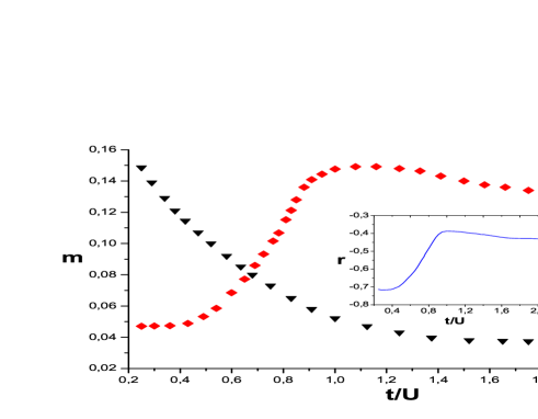
Figure 1: (Colour on-line) The effective spin of the itinerant electrons m as a function of the control parameter $t/U$-black triangles(left scale) The exchange constant $J/t$ as a function of $t/U$-red rhombuses(right scale). Inset: The effective anisotropy constant r as a function of $t/U$. The functions are calculated at density of itinerant electrons $n=0.4$, for anisotropy parameter $\kappa=-0.83$ and $J^{\prime}/t=10$.

For chosen parameters the exchange constant is positive $J>0$ and a ferromagnetic order along z axis, perpendicular to the anisotropy, is stable. To study this phase one introduces the Holstein-Primakoff representation of the spin vectors ${\bf M}_{j}(a^{+}_{j},\,a_{j})$

$$M_{j}^{+} = M_{j}^{x}+iM_{j}^{y}=\sqrt{2m-a_{j}^{+}a_{j}}\,a_{j}$$

$$M_{j}^{-} = M_{j}^{x}-iM_{j}^{y}=a_{j}^{+}\sqrt{2m-a_{j}^{+}a_{j}}$$

$$M_{j}^{3} = m-a_{j}^{+}a_{j},$$ (21)

where $a^{+}_{j},\,a_{j}$ are Bose fields and $m$ is the effective spin of itinerant electrons. In spin-wave approximation, in momentum space representation the effective Hamiltonian (Eq.20) adopts the form

$$h_{eff} = \sum\limits_{k}\left[\varepsilon_{k}a_{k}^{+}a_{k}\,-\,\gamma_{k}\left(a_{k}^{+}a_{-k}^{+}\,+\,a_{k}a_{-k}\right)\right]$$

$$\varepsilon_{k} = Jm\left[6-(1+r)\left(\cos k_{x}+\cos k_{y}+\cos k_{z}\right)\right]$$

$$\gamma_{k} = Jm\frac{(1-r)}{2}\left(\cos k_{x}+\cos k_{y}+\cos k_{z}\right).$$ (22)

To diagonalize the Hamiltonian one introduces new Bose field $\alpha_{k},\,\alpha_{k}^{+}$: $a_{k}\,=u_{k}\,\alpha_{k}\,+\,v_{k}\,\alpha^{+}_{-k}$, where the coefficients $u_{k}$ and $v_{k}$ are real functions of the wave vector. The transformed Hamiltonian adopts the form

$$h_{eff}=\sum\limits_{k}\left(E_{k}\,\alpha_{k}^{+}\alpha_{k}\,+\,E^{0}_{k}\right),$$ (23)

with dispersion

$$E_{k} = 2Jm\sqrt{\left(3-\delta_{k}\right)\left(3-r\delta_{k}\right)}$$

$$\delta_{k} = \cos k_{x}+\cos k_{y}+\cos k_{z}$$ (24)

and vacuum energy $E^{0}_{k}\,=\,\frac{1}{2}\,\left[E_{k}\,-\,\varepsilon_{k}\right]$.

The dispersion Eq.(Ferromagnetic Quantum critical behavior in three-dimensional Hubbard model with transverse anisotropy) shows that the ferromagnetism with magnetic order perpendicular to the anisotropy axis is stable if the effective anisotropy constant satisfies the condition $-1<r<1$. The inset in Fig.(1) shows that all calculated values of the effective anisotropy constant satisfy the above condition.

The dispersion is equal to zero at $\textbf{k}=(0,0,0)$. Therefor, $\alpha_{k}$-Boson describes long-range excitation (magnon) in the system. Near the zero vector the dispersion adopts the form $E_{k}\propto c_{s}|\textbf{k}|$ with spin-wave velocity

$$c_{s}=Jm\sqrt{6(1-r)}.$$ (25)

The unusual, for ferromagnetism, dispersion is in consequence of anisotropy. When the isotropy is restored ($r=1$) one obtains the well known ferromagnetic dispersion.

The magnetization is defined by the equation (Ferromagnetic Quantum critical behavior in three-dimensional Hubbard model with transverse anisotropy). At Curie temperature $T_{C}$, the magnetization is zero and one calculates the critical temperature solving the equation

$$2m+1=\frac{1}{N}\sum\limits_{k}\frac{\varepsilon_{k}}{E_{k}}\left[1+\frac{2}{e^{\frac{E_{k}}{T_{C}}}-1}\right].$$ (26)

When the parameter of anisotropy $r$ is fixed, the critical temperature decreases, decreasing the effective spin $m$. At quantum critical point ($T_{C}=0$) one obtains a dependence of the critical value of the effective spin $m_{cr}$ on the anisotropy parameter. The relation is given by the equation

$$2m_{cr}+1=\frac{1}{2N}\sum\limits_{k}\frac{6-(1+r)\delta_{k}}{\sqrt{(3-\delta_{k})(3-r\delta_{k})}}$$ (27)

with $\delta_{k}$ from Eq.(Ferromagnetic Quantum critical behavior in three-dimensional Hubbard model with transverse anisotropy), and is depicted in Fig(2).

Figure 2: (Colour on-line)  The effective spin $m_{cr}$, at quantum critical point, as a function of the effective parameter of anisotropy.

The figure (2) demonstrates very well the nature of the quantum criticality in itinerant ferromagnets with anisotropy. At quantum critical point the effective spin, which is the fermion contribution to the magnetization without accounting for the spin fluctuations, is nonzero. Magnon fluctuations suppress this magnetization to zero. Hence, the magnon (spin flip) fluctuations drive the system to quantum critical point. This is a second order quantum phase transition from ferromagnetic phase with long-range magnon fluctuations to paramagnetic phase with gapped magnons.

This is in contrast to quantum phase transition in isotropic itinerant ferromagnets ($r=1$). For this systems the quantum phase transition is from ferromagnetic phase with long-range magnon fluctuations to paramagnetic phase without spin-flip fluctuations ($m_{cr}=0$). This explains the non-second order nature of the transition.

Utilizing the dependence of the effective spin $m$ and the exchange constant $J/t$ on the control parameter $t/U$, see Fig. (1), one can obtain the dependence of the dimensionless temperature $T_{C}/t$ on the ration $t/U$. The phase diagram in the plane of temperature $T_{C}/t$ and control parameter $t/U$ is depicted in figure (3). At density of electrons $n=0.4$, anisotropy parameter $\kappa=-0.83$ and $J^{\prime}/t=10$ the quantum critical value of the ratio is $t/U=2$.

Figure 3: (Colour on-line)  The phase diagram in the plane of temperature $T_{C}/t$ and control parameter $t/U$. At density of electrons $n=0.4$, anisotropy parameter $\kappa=-0.83$ and $J^{\prime}/t=10$ the quantum critical value of the ratio is $t/U=2$.

In the present paper the Hubbard model of itinerant ferromagnetism with transverse anisotropy was studied. Increasing the ratio $t/U$ decreases the effective spin of itinerant electron which in turn decreases the Curie temperature. The equations (13) and (14) show that at fix density of electrons $n=0.4$ the decreasing of the effective spin increases the density of doubly occupied states. The result shows that the quantum critical ground state state is a state with high concentration of doubly occupied states.

This work was partly supported by a Grant-in-Aid DO02-264/18.12.08 from NSF-Bulgaria.

References

• (1) J. Hertz, Phys. Rev. B 14, 1165 (1976).
• (2) S. Sachdev, Quantum Phase Tramsition (Cambridge University Press,Cambridge 1999).
• (3) Matthias Vojta, Rep. Prog. Phys. 66 2069 (2003).
• (4) Hilbert v. LΓΆhneysen, Achim Rosch, Matthias Vojta, and Peter WΓΆlfle, Rev. Mod. Phys., 79, 1015 (2007).
• (5) Philipp Gegenwart, Qimiao Si, and Frank. Steglich, Nature Phys. 4 186 (2008).
• (6) A. J. Millis, Phys. Rev. B 48, 7183 (1993).
• (7) D. Bitko, T. F. Rosenbaum, and G. Aeppli, Phys. Rev. Lett. 77, 940 (1996).
• (8) S. SΓΌllow, M. C. Aronson, B. D. Rainford, and P. Haen, Phy. Rev. Lett. 82, 2963 (1999).
• (9) N. T. Huy, A. Gasparini, J. C. P. Klaasse, A. de Visser, S. Sakarya, and N. H. van Dijk, Phys.Rev. B 75, 212405 (2007).
• (10) E. C. Stoner, Proc.Roy.Soc.London A165, 372 (1938).
• (11) D. Belitz, T. R. Kirkpatrick, and T. Vojta, Phys. Rev. Lett. 82, 4707 (1999).
• (12) T. R. Kirkpatrick and D. Belitz, Phys. Rev. B 67, 024419 (2003).
• (13) Andrey V. Chubukov, Catherine PΓ©pin, and Jerome Rech, Phys. Rev. Lett. 92, 147003 (2004).
• (14) T. R. Kirkpatrick and D. Belitz, Phys. Rev. B 85, 134451 (2012).
• (15) D. Schmeltzer, Phys. Rev. B 43, 8650 (1991).