The flux calibration of Gaia

Abstract

The Gaia mission is described, along with its scientific potential and its updated science perfomancesAlthough it is often described as a self-calibrated mission, Gaia still needs to tie part of its measurements to external scales (or to convert them in physical units). A detailed decription of the Gaia spectro-photometric standard stars survey is provided, along with a short description of the Gaia calibration model. The model requires a grid of approximately 200 stars, calibrated to a few percent with respect to Vega, and covering different spectral types.

1 The Gaia mission

Gaia is a cornerstone mission of the ESA Space Program, presently scheduled for launch in 2013. The Gaia satellite will perform an all-sky survey to obtain parallaxes and proper motions to $\mu as$ precision for about 10⁹ point-like sources and astrophysical parameters ($T_{\mathrm{eff}}$, $\log g$, $E(B-V)$, metallicity etc.) for stars down to a limiting magnitude of $V\simeq 20$, plus 2-30 km/s accuracy (depending on spectral type), radial velocities for several millions of stars down to $V<17$.

Such an observational effort has been compared to the mapping of the human genome for the amount of collected data and for the impact that it will have on all branches of astronomy and astrophysics. The expected end-of-mission astrometric accuracies are almost 100 times better than the Hipparrcos dataset (see Perryman et al. 1997). This exquisite precision will allow a full and detailed reconstruction of the 3D spatial structure and 3D velocity field of the Milky Way galaxy within $\simeq 10$ kpc from the Sun. This will provide answers to long-standing questions about the origin and evolution of our Galaxy, from a quantitative census of its stellar populations, to a detailed characterization of its substructures (as, for instance, tidal streams in the Halo, see Ibata & Gibson 2007), to the distribution of dark matter.

The accurate 3D motion of more distant Galactic satellites (as globular clusters and the Magellanic Clouds) will be also obtained by averaging the proper motions of many thousands of member stars: this will provide an unprecedented leverage to constrain the mass distribution of the Galaxy and/or non-standard theories of gravitation. Gaia will determine direct geometric distances to essentially any kind of standard candle currently used for distance determination, setting the whole cosmological distance scale on extremely firm bases.

As challenging as it is, the processing and analysis of the huge data-flow incoming from Gaia is the subject of thorough study and preparatory work by the Data Processing and Analysis Consortium (DPAC), in charge of all aspects of the Gaia data reduction. The consortium comprises more than 400 scientists from 25 European institutes. Gaia is usually described as a self-calibrating mission, but it also needs external data to fix the zero-point of the magnitude system and radial velocities, and to calibrate the classification/parametrization algorithms. All these additional data are termed auxiliary data and have to be available, at least in part, three months before launch. While part of the auxiliary data already exist and must only be compiled from archives, this is not true for several components. To this aim a coordinated programme of ground-based observations is being organized by a dedicated inter-CU committee (GBOG), that promotes sinergies and avoids duplications of effort.

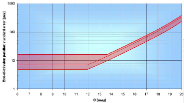
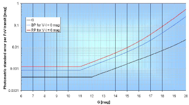
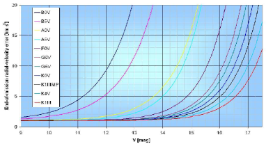
Figure 1.: The Gaia updated science performances. Top left panel: The end-of-mission uncertainty on astrometric measurements (in $\mu$as) as a function of the integrated G magnitude of a G2V star. Top right panel: End-of-mission uncertainties on the G, G_BP, G_RP magnitudes as a function of G, for a V–I=0 mag star. Bottom left panel: End-of-mission uncertainty on radial velocity (in km/s) as a function of G magnitude for different spectral types. Bottom right panel: Uncertainty on the metallicity ([M/H] in dex) derived from RVS spectra as a function of the S/N ratio for different Galactic populations. ©ESA

1.1 Science goals and capabilities

Gaia will measure the positions, distances, space motions, and many physical characteristics of some billion stars in our Galaxy and beyond. For many years, the state of the art in celestial cartography has been the Schmidt surveys of Palomar and ESO, and their digitized counterparts. The measurement precision, reaching a few millionths of a second of arc, will be unprecedented. The most updated science performances can be found on the Gaia ESA webpage, along with some formulaes to re-compute figures easily, and with all the references (see Fig. 1). Some millions of stars will be measured with a distance accuracy of better than 1 per cent; some 100 million or more to better than 10 per cent. Gaia’s resulting scientific harvest is of almost inconceivable extent and implication.

Gaia will provide detailed information on stellar evolution and star formation in our Galaxy. It will clarify the origin and formation history of our Galaxy. The results will precisely identify relics of tidally-disrupted accretion debris, probe the distribution of dark matter, establish the luminosity function for pre-main sequence stars, detect and categorize rapid evolutionary stellar phases, place unprecedented constraints on the age, internal structure and evolution of all stellar types, establish a rigorous distance scale framework throughout the Galaxy and beyond, and classify star formation and kinematical and dynamical behaviour within the Local Group of galaxies.

Gaia will pinpoint exotic objects in colossal and almost unimaginable numbers: many thousands of extra-solar planets will be discovered (from both their astrometric wobble and from photometric transits) and their detailed orbits and masses determined; tens of thousands of brown dwarfs and white dwarfs will be identified; tens of thousands of extragalactic supernovae will be discovered; Solar System studies will receive a massive impetus through the observation of hundreds of thousands of minor planets; near-Earth objects, inner Trojans and even new trans-Neptunian objects, including Plutinos, may be discovered.

Gaia will follow the bending of star light by the Sun and major planets over the entire celestial sphere, and therefore directly observe the structure of space-time – the accuracy of its measurement of General Relativistic light bending may reveal the long-sought scalar correction to its tensor form. The PPN parameters $\gamma$ and $\beta$, and the solar quadrupole moment J2, will be determined with unprecedented precision. All this, and more, through the accurate measurement of star positions.

For more information on the Gaia mission: http://www.rssd.esa.int/Gaia. More information for the public on Gaia and its science capabilities are contained in the Gaia information sheets. Excellent reviews of the science possibilities opened by Gaia can be found in Perryman et al. (1997) and Mignard (2005).

1.2 Launch, timeline and data releases

The first idea for Gaia began circulating in the early 1990, culminating in a proposal for a cornerstone mission within ESA’s science programme submitted in 1993, and a workshop in Cambridge in June 1995. By the time the final catalogue will be released approximately in 2020, almost two decades of work will have elapsed between the orginal concept and mission completion.

Gaia will be launched by a Soyuz carrier (rather than the initially foreseen Ariane 5) in 2013 from French Guyana and will start operating once it will reach its Lissajus orbit around L2 (the unstable Langrange point of the Sun and Eart-Moon system), in about one month. Two ground stations will receive the compressed Gaia data during the 5 years of operation: Cebreros (Spain) and Perth (Australia). The data will then be transmitted to the main data centers throughout Europe to allow for data processing. We are presently in technical development phase C/D, and the hardware is being built, tested and assembled. Software development started in 2006 and is presently producing and testing pipelines with the aim of delivering to the astrophysical community a full catalogue and dataset ready for scientific investigation.

Apart from the end-of-mission data release, foreseen around 2020, some intermediate data releases are foreseen. In particular, there should be one first intermediate release covering either the first 6 months or the first year of operation, followed by a second and possibly a third intermediate release, that are presently being discussed. The data analysis will proceed in parallel with observations, the major pipelines re-processing all the data every 6 months, with secondary cycle pipelines – dedicated to specific tasks – operating on different timescales. In particular, verified science alerts, based on unexpected variability in flux and/or radial velocity, are expected to be released within 24 hours from detection, after an initial period of testing and fine-tuning of the detection algorithms.

1.3 Mission concepts

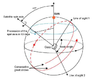
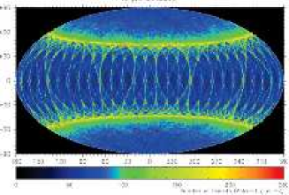
Figure 2.: Left: the scanning law of Gaia during main operations; Right: the average number of passages on the sky, in ecliptic coordinates. ©ESA

During its 5-year operational lifetime, the satellite will continuously spin around its axis, with a constant speed of 60 arcsec/sec. As a result, over a period of 6 hours, the two astrometric fields of view will scan across all objects located along the great circle perpendicular to the spin axis (Figure 2). As a result of the basic angle of 106.5^o separating the astrometric fields of view on the sky, objects transit the second field of view with a delay of 106.5 minutes compared to the first field. Gaia’s spin axis does not point to a fixed direction in space, but is carefully controlled so as to precess slowly on the sky. As a result, the great circle that is mapped by the two fields of view every 6 hours changes slowly with time, allowing reapeated full sky coverage over the mission lifetime. The best strategy, dictated by thermal stability and power requirements, is to let the spin axis precess (with a period of 63 days) around the solar direction with a fixed angle of 45^o. The above scanning strategy, referred to as “revolving scanning”, was successfully adopted during the Hipparcos mission.

Every sky region will be scanned on average 70-80 times, with regions lying at $\pm$45^o from the Ecliptic Poles being scanned on average more often than other locations. Each of the Gaia targets will be therefore scanned (within differently inclined great circles) from a minimum of approximately 10 times to a maximum of 250 times (Figure 2, right panel). Only point-like sources will be observed, and in some regions of the sky, like the Baade’s window, $\omega$ Centauri or other globular clusters, the star density of the two combined fields of view will be of the order of 750 000 or more per square degree, exceeding the storage capability of the onboard processors, so Gaia will not study in detail these dense areas.

1.4 Focal plane

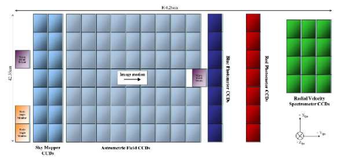
Figure 3.: The 105 on the Gaia focal plane. ©ESA

Figure 3 shows the focal plane of Gaia, with its 105 CCDs, which are read in TDI (Time Delay Integration) mode: objects enter the focal plane from the left and cross one CCD in 4 seconds. Apart from some technical CCDs that are of little interest in this context, the first two CCD columns, the Sky Mappers (SM), perform the on-board detection of point-like sources, each of the two columns being able to see only one of the two lines of sight. After the objects are identified and selected, small windows are assigned, which follow them in the astrometric field (AF) CCDs where white light (or G-band) images are obtained (Section 1.5). Immediately following the AF, two additional columns of CCDs gather light from two slitless prism spectrographs, the blue spectrophotometer (BP) and the red one (RP), which produce dispersed images (Section 1.6). Finally, objects transit on the Radial Velocity Spectrometer (RVS) CCDs to produce higher resolution spectra around the Calcium Triplet (CaT) region (Section 1.7).

1.5 Astrometry

The AF CCDs will provide G-band images, i.e., white light images where the passband is defined by the telescope optics transmission and the CCDs sensitivity, with a very broad combined passband ranging from 330 to 1050 nm and peaking around 500–600 nm (Figure 4). The objective of Gaia’s astrometric data reduction system is the construction of core mission products: the five standard astrometric parameters, position ($\alpha$, $\delta$), parallax ($\varpi$), and proper motion ($\mu_{\alpha}$, $\mu_{\delta}$) for all observed stellar objects. The expected end-of-mission precision is shown in Figure 1 and discussed in detail in the Gaia ESA webpages.

To reach these end-of-mission precisions, the average 70–80 observations per target gathered during the 5-year mission duration will have to be combined in a self-consistent manner. 40 Gb of telemetry data will first pass through the Initial Data Treatment (IDT) which determines the image parameters and centroids, and then performes an object cross-matching. The output forms the so-called One Day Astrometric Solution (ODAS), together with the satellite attitude and calibration, to the sub-milliarcsecond accuracy. The data are then written to the Main Database.

The next step is the Astrometric Global Iterative Solution (AGIS) processing. AGIS processes together the attitude and calibration parameters with the source parameters, refining them in an iterative procedure that stops when the adjustments become sufficiently small. As soon as new data come in, on the basis of 6 months cycles, all the data in hand are reprocessed toghether from scratch. This is the only scheme that allows for the quoted precisions, and it is also the philosophy that justifies Gaia as a self-calibrating mission. The primary AGIS cycle will treat only stars that are flagged as single and non-variable (expected to be around 500 millions), while other kinds of objects will be computed in secondary AGIS cycles that utilize the main AGIS solution. Dedicated pipelines for specific kinds of objects (asteroids, slightly extended objects, variable objects and so on) are being put in place to extract the best possible precision. Owing to the large data volume (100 Tb) that Gaia will produce, and to the iterative nature of the processing, the computing challenges are formidable: AGIS processing alone requires some 10²¹ FLOPs which translates to runtimes of months on the ESAC computers in Madrid.

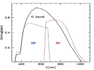
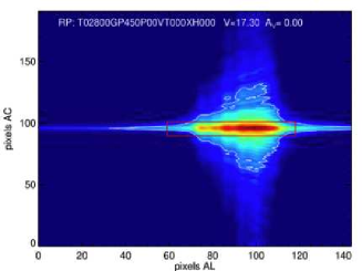
Figure 4.: Left: the passbands of the G-band, BP and RP; Right: a simulated RP dispersed image, with a red rectangle marking the window assigned for compression and ground telemetry. ©ESA

1.6 Spectrophotomety

The primary aim of the photometric instrument is mission critical in two respects: (i) to correct the measured centroids position in the AF for systematic chromatic effects, and (ii) to classify and determine astrophysical characteristics of all objects, such as temperature, gravity, mass, age and chemical composition (in the case of stars).

The BP and RP spectrophotometers are based on a dispersive-prism approach such that the incoming light is not focussed in a PSF-like spot, but dispersed along the scan direction in a low-resolution spectrum. The BP operates between 330–680 nm while the RP between 640-1000 nm (Figure 4). Both prisms have appropriate broad-band filters to block unwanted light. The two dedicated CCD stripes cover the full height of the AF and, therefore, all objects that are imaged in the AF are also imaged in the BP and RP.

The resolution is a function of wavelength, ranging from 4 to 32 nm/pix for BP and 7 to 15 nm/pix for RP. The spectral resolution, R=$\lambda/\delta\lambda$ ranges from 20 to 100 approximately. The dispersers have been designed in such a way that BP and RP spectra are of similar sizes (45 pixels). Window extensions meant to measure the sky background are implemented. To compress the amount of data transmitted to the ground, all the BP and RP spectra – except for the brightest stars – are binned on chip in the across-scan direction, and are transmitted to the ground as one-dimensional spectra. Figure 4 shows a simulated RP spectrum, unbinned, before windowing, compression, and telemetry.

The final data products will be the end-of-mission (or intermediate releases) of global, combined BP and RP spectra and integrated magnitudes G_BP and G_RP. Epoch spectra will be released only for specific classes of objects, such as variable stars and quasars, for example. The internal flux calibration of integrated magnitudes, including the G magnitudes as well, is expected at a precision of 0.003 mag for G=13 stars, and for G=20 stars goes down to 0.07 mag in G, 0.3 mag in G_BP and G_RP. The external calibration should be performed with a precision of the order of a few percent (with respect to Vega, see section 4).

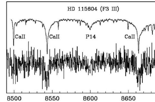
Figure 5.: Simulated RVS end-of-mission spectra for the extreme cases of 1 single transit (bottom spectrum) and of 350 transits (top spectrum). ©ESA

1.7 High-resolution spectroscopy

The primary objective of the RVS is the acquisition of radial velocities, which combined with positions, proper motions, and parallaxes will provide the means to decipher the kinematical state and dynamical history of our Galaxy.

The RVS will provide the radial velocities of about 100–150 million stars up to 17-th magnitude with the precisions illustrated in Figure 1 and in the Gaia ESA webpage. The spectral resolution, R=$\lambda$/$\delta\lambda$ will be 11 500. Radial velocities will be obtained by cross-correlating observed spectra with either a template or a mask. An initial estimate of the source atmospheric parameters will be used to select the most appropriate template or mask. On average, 40 transits will be collected for each object during the 5-year lifetime of Gaia, since the RVS does not cover the whole width of the Gaia AF (Figure 3). In total, we expect to obtain some 5 billion spectra (single transit) for the brightest stars. The analysis of this huge dataset will be complicated, not only because of the sheer data volume, but also because the spectroscopic data analysis relies on the multi-epoch astrometric and photometric data.

The covered wavelength range (847-874 nm, Figure 5) is a rich domain, centered on the infrared calcium triplet: it will not only provide radial velocities, but also many stellar and interstellar diagnostics. It has been selected to coincide with the energy distribution peaks of G anf K type stars, which are the most abundant targets. In early type stars, RVS spectra may contain also weak He lines and N, although they will be dominated by the Paschen lines. The RVS data will effectively complement the astrometric and photometric observations, improving object classification. For stellar objects, it will provide atmospheric parameters such as effective temperature, surface gravity, and individual abundances of key elements such as Fe, Ca, Mg, Si for millions of stars down to G$\simeq$12. Also, Diffuse Intertellar Bands (DIB) around 862 nm will enable the derivation of a 3D map of interstellar reddening.

2 Flux calibration model

Calibrating (spectro)photometry obtained from the usual type of ground based observations (broadband imaging, spectroscopy) is not a trivial task, but the procedures are well known (see, e.g., Bessell 1999) and many groups have developed sets of appropriate standard stars for the more than 200 photometric known systems, and for spectroscopic observations.

In the case of Gaia, several instrumental effects – much more complex than those usually encountered – redistribute light along the SED (Spectral Energy Distribution) of the observed objects. The most difficult Gaia data to calibrate are the BP and RP slitless spectra, requiring a new approach to the derivation of the calibration model and to the SPSS grid needed to perform the actual calibration. Some important complicating effects are:

• the large focal plane with its large number of CCDs makes it so that different observations of the same star will be generally on different CCDs, with different quantum efficiencies, optical distorsions, transmissivity and so on. Therefore, each wavelength and each position across the focal plane has its (sometimes very different) PSF (point spread function);

• TDI (Time Delayed Integration) continuous reading mode, combined with the need of compressing most of the data before on-ground transmission, make it necessary to translate the full PSF into a linear (compressed into 1D) LSF (Line Spread Function), which of course adds complication into the picture;

• in-flight instrument monitoring is foreseen, but never comparable to the full characterization that will be performed before launch, so the real instrument – at a certain observation time – will be slightly different from the theoretical one assumed initially, and this difference will change with time;

• finally, radiation damage (or CTI, Charge Transfer Inefficiencies) deserves special mention, for it is one of the most important factors in the time variation of the instrument model (Weiler et al. 2011; Prod’Homme 2011). It has particular impact onto the BP and RP dispersed images because the objects travel along the BP and RP CCD strips in a direction that is parallel to the spectral dispersion (wavelength coordinate) and therefore the net effect of radiation damage can be to alter the SED of some spectra. Several solutions are being tested to mitigate CTI effects, but the global instrument complexity calls for a new approach to spectra flux calibrations.

A flux calibration model is currently implemented in the photometric pipeline, which splits the calibration into an internal and an external part. The internal calibration model (Jordi 2011) uses a large number of well behaved stars (internal standards), observed by Gaia, to report all observations to a reference instrument, on the same instrumental relative flux and wavelength scales. Once each observation for each object is reported to the internal reference scales, the absolute or external calibration (Montegriffo & Bellazzini 2009; Ragaini et al. 2011) will use an appropriate SPSS set to report the relative flux scale to an absolute flux scale in physical units, tied to the calibration of Vega (see also Section 3). Alternative approaches, where the internal and external calibration steps are more inter-connected, are being tested to maximise the precision and the accuracy of the Gaia calibration (Brown et al. 2010). The Gaia calibration model was also described by Pancino (2010), Jordi (2011), and Cacciari (2011).

The final flux calibrated products will be: averaged (on all transits – or observations) white light magnitudes, G; integrated BP/RP magnitudes, G_BP and G_RP; flux calibrated BP/RP spectra; RVS spectra and integrated G_RVS magnitudes, possibly also flux calibrated. The G_BP–G_RP colour will be used to correct for chromaticity effects in the global astrometric solution. As said, only for specific classes of objects, epoch spectra and magnitudes will be released, with variable stars as an obvious example.

The external calibration model contains – as discussed – a large number of parameters, requiring a large number (about 200) of calibrators. With the standard calibration techniques (Bessell 1999), the best possible calibrators are hot, almost featureless stars such as WD or hot subdwarfs. Unfortunately, these stars are all similar to each other, forming an intrinsically degenerate set. The Gaia calibration model instead requires to differentiate as much as possible the calibrators, by including smooth spectra, but also spectra with absorption features, both narrow (atomic lines) or wide (molecular bands), appearing both on the blue and the red side of the spectrum. An experiment described by Pancino (2010) shows that the inclusion of just a few M stars with large molecular absorptions in the Gaia SPSS set can improve the calibration of similarly red stars by a factor of more than ten (from a formal error of 0.15 mag to an error smaller than 0.01 mag).

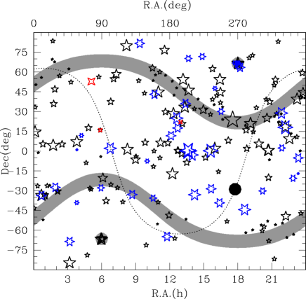
Figure 6.: Distribution of our SPSS candidates on the sky. The Galactic plane and center are marked with a dotted line and a large black circle, respectively. The Ecliptic poles are marked as two large grey circles, and two stripes at $\pm$45 deg from the Ecliptic poles (roughly where Gaia is observing more often) are shaded in grey. Our Pillars are shown as three four-pointed stars, the Primary SPSS candidates as six-pointed stars, and the Secondary SPSS candidates as five-pointed stars. The stars size is proportional to the SPSS brightness, ranging from V$\simeq$8 (largest symbols) to 15 mag (smallest symbols), approximately.

In conclusion, the complexity of the instrument reflects in a complex calibration model, that requires a large set of homogeneously calibrated SPSS, covering a range of spectral types. No such database exists in the literature, and new observations are necessary to build it.

3 The Gaia grid of spectrophotometric standard stars

From the above discussion, it is clear that the Gaia SPSS grid has to be chosen with great care. The Gaia SPSS, or better their reference flux tables should conform to the following general requirements (van Leeuven et al. 2010):

• Resolution R=$\lambda/\delta\lambda\simeq 1000$, i.e., they should oversample the Gaia BP/RP resolution by a factor of 4–5 at least;

• Wavelength coverage: 330–1050 nm;

• Typical uncertainty on the absolute flux scale, with respect to the assumed calibration of Vega, of a few percent, excluding small troubled areas in the spectral range (telluric bands residuals, extreme red and blue edges), where it can be somewhat worse.

The total number of SPSS in the Gaia grid should be of the order of 200–300 stars, including a variety of spectral types. Clearly, no such large and homogeneous dataset exists in the literature yet. It is therefore necessary to build the Gaia SPSS grid with new, dedicated observations. We describe the characteristics of the Gaia SPSS and of the dedicated observing campaigns in the following Sections.

3.1 SPSS Candidates

We have followed a two steps approach (Bellazzini et al. 2006) that firstly creates a set of Primary SPSS, i.e., well known SPSS that are calibrated on the three Pillars of the CALSPEC set, described in Bohlin et al. (1995) and Bohlin (2007), and tied to the Vega flux calibration by Bohlin & Gilliland (2004) and Bohlin (2007). The Primary SPSS (Altavilla et al. 2008) will constitute the ground-based calibrators of the actual Gaia grid, and need to be suitably bright for 2–4 m class telescopes in both hemispheres. The most important sources for Primary candidates are the CALSPEC grid, Oke (1990), Hamuy et al. (1992, 1994), Stritzinger et al. (2005) and others.

The Secondary SPSS (Altavilla et al. 2010) will form, together with the eligible primaries, the actual Gaia SPSS grid and will conform to the following requirements (van Leeuwen et al. 2011):

• Secondary SPSS have spectra as featureless as possible (but see below for exceptions);

• Secondary SPSS shall be validated against variability;

• The magnitude and sky location (i.e., number of useful, clean transits, see Carrasco et al. 2010, 2007) of Secondary SPSS grants a resulting S/N$\simeq$100 per sample over most of the wavelength range when observed by Gaia (end of mission);

• Secondary SPSS cover a range of spectral types and spectral shapes, as needed to ensure the best possible claibration of all kinds of objects observed by Gaia.

Additional, special members of the Secondary SPSS candidates are: (1) a few selected SPSS around the Ecliptic Poles, two regions of the sky that will be repeatedly observed by Gaia, in the first two weeks after reaching its orbit in L2, for calibration purposes; (2) a few M stars with deep absorption features in the red; (3) a few SDSS stars that have been observed in SEGUE sample (Yanny et al. 2009; Bellazzini et al. 2010); (4) a few well known SPSS that are among the targets of the ACCESS mission (Kaiser et al. 2010), dedicated to the absolute flux measurement of a few stars besides Vega.

4 The Gaia SPSS survey

Our survey is split into two campaigns, the main campaign dedicated to obtaining spectrophotometry of all our candidate SPSS, and the auxiliary campaign dedicated to monitoring the constancy of our SPSS on relevant timescales.

• Main campaign. Classical spectrophotometry (Bessell 1999) would clearly be the best approach to obtain absolutely calibrated flux spectra if we had a dedicated telescope. However tihs approach would require too much time, given that we need high S/N of 300 stars, in photometric sky conditions, which are rare. We thus decided for a combined approach, in which spectra are obtained even if the sky is non-photometric, providing the correct spectral shape of our SPSS. Then, imaging in photometric conditions and in three bands (generally B, V, and R, but sometimes also I and, more rarely, U) is obtained and calibrated magnitudes are used to scale the spectra to the correct zeropoint.

• Constancy monitoring. Even stars used for years as spectrophotometric standards were found to vary when dedicated studies have been performed (see e.g., G24-9, that was found to be an eclipsing binary by Landolt & Uomoto 2007); our own survey has already found a few variables, including one of the CALSPEC standards (Section 5.1). White dwarfs may show variability with (multi-)periods from about 1 to 20 min and amplitudes from about 1-2% up to 30%, i.e., ZZ Ceti type variability. We have tried to exclude stars within the instability strips for DAV (Castanheira et al. 2007), DBV, and DOV but in many cases the existing information was not sufficient (or sufficiently accurate) to firmly establish the constant nature of a given WD. Also redder stars are often found to be variable: for example K stars have shown variability of 5-10% with periods of the order 1–10 days (Eyer & Grenon 1997). In addition, eclipsing binaries are frequent and can be found at all spectral types. Their periods can range from a few hours to hundreds of days, most of them having $P\simeq$ 1-10 days, (Dvorak 2004).

Our chosen observing facilities are imagers and low-resolution spectrographs in both hemispheres: EFOSC2@NTT and ROSS@REM at the ESO La Silla Observatory, Chile; CAFOS@2.2m at the Calar Alto Observatory, Spain; DOLORES@TNG at the Roque de Los Muchachos in La Palma, Spain; LaRuca@1.5m at the San Pedro Mártir Observatory, Mexico; BFOSC@Cassini in Loiano, Italy. Observations are almost complete — at the time of writing — only the long-term (3 yr) monitoring will be ongoing after Summer 2012, and is expected to finish in 2013-2014.

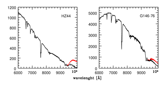
Figure 7.: Second-order contamination on DOLoRes@TNG spectra of a blue star (left panel) and a red star (right panel); the black lines are the corrected spectra, while the red lines above, starting at about 9500 Å, show the contaminated spectra.

5 Data treatment and data products

The required precision and accuracy of the SPSS calibration imposes the adoption of strict protocols of instrument characterization, data reduction, quality control, and data analysis. In particular, we carried out a detailed characterization of the intruments used:

• CCD familiarization plan, containing a study of the dark and bias frames stability; the shutter characterization (shutter times and delays); and the study of the linearity of all employed CCDs;

• Instrument familiarization plan studying the stability of imaging and spectroscopy flats, the study of fringing, and the lamp flexures of the employed spectrographs;

• Site familiarization plan, providing extinction curves, extinction coefficients, colour terms, and a study of the effect of “calima” on the spectral shape.

As a results of these studies, specific recommendations for observations and data treatment were defined. Data reductions are being performed mostly with IRAF and IRAF-based pipelines. We also use SExtractor (Bertin & Arnouts 1996) for aperture photometry, because it provides many useful parameters that we will use for a semi-automated quality control (QC) of each reduced frame.

To illustrate a detail of the reduction procedures, we show in Figure 7 our second-order contamination correction for a blue and a red star. The effect arises when light from blue wavelengths, from the second dispersed order of a particular grism or grating, falls on the red wavelengths of the first dispersed order. Such contamination usually happens when the instrument has no cross-disperser. Of the instruments we use, only EFOSC2@NTT and DOLoRes@TNG present significant contamination. To map the blue light falling onto our red spectra, we adapted a method proposed by Sánchez-Blázquez et al. (2006) and applied it to dedicated observations. Our wavelength maps generally allow to recover the correct spectral shape with residuals within $\pm$2%, as tested on a few CALSPEC standards observed with both TNG and NTT.

As an example of the final data quality, we show in Figure 8 a test performed to refine our reduction procedures, where a portion of the spectrum of HZ44 observed in a photometric night is compared with the CALSPEC flux table. We point out that this was just a preliminary reduction, where fringing and telluric absorption features were not properly removed yet. Even with these limitations, we were able to meet the requirements, because the residuals between our spectrum and the CALSPEC tabulated one were on average lower than 1%, with the exception of the low S/N red edge and of the telluric absorption bands. However, some unsatisfactory jumps appeared in the comparison, between 4000 and 6000 Å, where our spectra have the highest S/N. As shown in Figure 8 (top panel) and already noted by Bohlin et al. (2001), the jumps were due to a (minor) problem in the CALSPEC spectrum, probably where two pieces of the spectrum were joined.

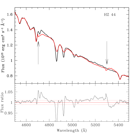
Figure 8.: Top panel: comparison of our preliminary spectrum of HZ 44 (thick black line) with the CALSPEC tabulated spectrum (thick red line) in a region where we found a discrepancy (marked by the two arrows), where small $\simeq$0.5–1.0% jumps in the CALSPEC spectrum are probably due to a mismatch of two different spectra. Bottom panel: ratio between our spectrum and the CALSPEC spectrum; perfect agreement (red line) and $\pm$1% agreement (dotted red lines, our requirement) are marked.

5.1 Preliminary results

During the years, we have cleaned our initial linelists (Altavilla et al. 2008, 2010) from unsuitable stars. On the one hand we kept our literature information updated, and to look for new about variability, activity, close companions and misidentification. On the other hand we used our own data to test the validity of each candidate.

Identification problems are common, especially when large databases are automatically matched (as done within SIMBAD, for example), and when stars have large proper motions. We found a few wrong identifications, the most notable case being that of LTT 377, which showed an F type spectrum rather than the expected K, and was in many databases confused with star CD -34 241, which corresponds to CD -34 239. A similar case was WD 0204-306 for which we obtained an unexpectedly red spectrum, corresponding to that of star LP 885-23, uncorrectly identified with WD 0204-306, while it is instead LP 885-22. A more critical example was WD 1148-230, having very different coordinates in the McCook & Sion (1999) catalogue (coming from Stys et al. 2000) and in SIMBAD. The SIMBAD coordinates were from the 2MASS catalogue (Cutri et al. 2003). Magnitudes were also significantly different, so we had to reject the candidate.

In a few cases candidates that appeared relatively isolated on the available finding charts turned out to be in a crowded area where no aperture photometry or reliable wide slit spectroscopy could be performed from the ground, or showed previously unseen companions. Generally, stars with high proper motion could appear isolated in some past finding chart, but later moved too close to another star to be safely observed from the ground. Examples of candidates showing the presence of previously unknown and relatively bright companions were WD 0406+592 and WD 2058+181. Both stars were rejected.

Figure 9.: Our best lightcurve for the CALSPEC standard 1740346 (obtained with BFOSC in Loiano on 1 September 2010), originally one of our Primary SPSS candidates. The average of all field-stars magnitude differences (i.e., zero) is marked with a solid line, while the $\pm$1, 2, and 3 $\sigma$ variations are marked with dotted lines.

Finally, star 1740346, one of the currently used CALSPEC standards and one of our Primary SPSS candidates, showed variability with an amplitude of 10 $\pm$ 0.8 mmag in B band when observed with BFOSC@Cassini in Loiano, on 1 September 2010; with DOLoRes@TNG, on 31 September 2009; and with BFOSC@Cassini, on 26 May 2009. The variability period is 50 min, approximately. A preliminary determination of 1740346 parameters can be found in Marinoni (2011), using literature data and stellar models, resulting in a mass of $\simeq$1.3 M_⊙, an effective temperature of $\simeq$8300 K, and a distance of $\simeq$750 pc. These parameters are also compatible with a $\delta$ Scuti type star. We are gathering detailed follow-up observations for a complete characterization of star 1740346. Our best differential lightcurve is presented in Figure 9.

6 Summary and conclusions

The Gaia mission and its data reduction is a challenging enterprise, carried on by ESA and the European scientific community. An even more challenging enterprise will be the scientific interpretation of such a large database, and the creation of tools which can efficiently explore it.

As an example of the DPAC (Data Processing and Analysis Consortium) tasks, I have briefly described the Gaia flux calibration model and the Gaia SPSS survey, which will build a large ($\simeq 200-300$) grid of SPSS with 1–3% flux calibration with respect to Vega. All data products will be eventually made public together with each Gaia data release, within the framework of the DPAC publication policies. At the moment the accumulated data and literature information are stored locally and can be accessed upon request.

References

- Altavilla et al. (2008) Altavilla, G., Bellazzini, M., Pancino, E., Bragaglia, A., Cacciari, C., Diolaiti, E., Federici, L., Montegriffo, P., & Rossetti, E. 2008, Primary standards for the establishment of the Gaia grid of SPSS. Selection criteria and list of candidates., Tech. Rep. GAIA-C5-TN-OABO-GA-001
- Altavilla et al. (2010) Altavilla, G., Bragaglia, A., Pancino, E., Bellazzini, M., Cacciari, C., Federici, L., & Ragaini, S. 2010, Secondary standards for the establishment of the Gaia grid of SPSS. Selection criteria and list of candidates., Tech. Rep. GAIA-C5-TN-OABO-GA-003
- Bellazzini et al. (2010) Bellazzini, M., Altavilla, G., & Cacciari, C. 2010, Notes on the possible use of SEGUE spectrophotometry for the absolute photometric calibration of Gaia., Tech. Rep. GAIA-C5-TN-OABO-MBZ-002
- Bellazzini et al. (2006) Bellazzini, M., Bragaglia, A., Federici, L., Diolaiti, E., Cacciari, C., & Pancino, E. 2006, Absolute calibration of Gaia photometric data. I. General considerations and requirements., Tech. Rep. GAIA-C5-TN-OABO-MBZ-001
- Bertin & Arnouts (1996) Bertin, E., & Arnouts, S. 1996, A&AS, 117, 393
- Bessell (1999) Bessell, M. S. 1999, PASP, 111, 1426
- Bohlin (2007) Bohlin, R. C. 2007, in The Future of Photometric, Spectrophotometric and Polarimetric Standardization, edited by C. Sterken, vol. 364 of Astronomical Society of the Pacific Conference Series, 315. arXiv:astro-ph/0608715
- Bohlin et al. (1995) Bohlin, R. C., Colina, L., & Finley, D. S. 1995, AJ, 110, 1316
- Bohlin et al. (2001) Bohlin, R. C., Dickinson, M. E., & Calzetti, D. 2001, AJ, 122, 2118
- Bohlin & Gilliland (2004) Bohlin, R. C., & Gilliland, R. L. 2004, AJ, 127, 3508
- Brown et al. (2010) Brown, A., Jordi, C., & Fabricius, C. 2010, Forward modeling of the BP/RP data processing: options and implications., Tech. Rep. GAIA-C5-TN-LEI-AB-020
- Cacciari (2011) Cacciari, C. 2011, in EAS Publications Series, vol. 45 of EAS Publications Series, 155
- Carrasco et al. (2010) Carrasco, J. M., Jordi, C., Figueras, A. G., F., & B., A. E. 2010, Towards the selection of standard stars for absolute flux calibration. Signal-to-noise ratios for BP/RP spectra and crowding due to FoV overlapping., Tech. Rep. GAIA-C5-TN-UB-JMC-001
- Carrasco et al. (2007) Carrasco, J. M., Jordi, C., Lopez-Marti, B., Figueras, F., & Anglada-Escude, G. 2007, Revolving phase effct to FoV overlapping and its application to primary SPSS., Tech. Rep. GAIA-C5-TN-UB-JMC-002
- Castanheira et al. (2007) Castanheira, B. G., Kepler, S. O., Costa, A. F. M., Giovannini, O., Robinson, E. L., Winget, D. E., Kleinman, S. J., Nitta, A., Eisenstein, D., Koester, D., & Santos, M. G. 2007, A&A, 462, 989. arXiv:astro-ph/0611332
- Cutri et al. (2003) Cutri, R. M., Skrutskie, M. F., van Dyk, S., Beichman, C. A., Carpenter, J. M., Chester, T., Cambresy, L., Evans, T., Fowler, J., Gizis, J., et al. 2003, VizieR Online Data Catalog, 2246, 0
- Dvorak (2004) Dvorak, S. W. 2004, Information Bulletin on Variable Stars, 5542, 1
- Eyer & Grenon (1997) Eyer, L., & Grenon, M. 1997, in Hipparcos - Venice ’97, edited by R. M. Bonnet, E. Høg, P. L. Bernacca, L. Emiliani, A. Blaauw, C. Turon, J. Kovalevsky, L. Lindegren, H. Hassan, M. Bouffard, B. Strim, D. Heger, M. A. C. Perryman, & L. Woltjer, vol. 402 of ESA Special Publication, 467
- Eyer & Mowlavi (2008) Eyer, L., & Mowlavi, N. 2008, Journal of Physics Conference Series, 118, 012010. 0712.3797
- Hamuy et al. (1994) Hamuy, M., Suntzeff, N. B., Heathcote, S. R., Walker, A. R., Gigoux, P., & Phillips, M. M. 1994, PASP, 106, 566
- Hamuy et al. (1992) Hamuy, M., Walker, A. R., Suntzeff, N. B., Gigoux, P., Heathcote, S. R., & Phillips, M. M. 1992, PASP, 104, 533
- Ibata & Gibson (2007) Ibata, R., & Gibson, B. 2007, Scientific American, 296, 040000
- Jordi (2011) Jordi, C. 2011, in EAS Publications Series, vol. 45 of EAS Publications Series, 149
- Kaiser et al. (2010) Kaiser, M. E., Kruk, J. W., McCandliss, S. R., Rauscher, B. J., Kimble, R. A., Pelton, R. S., Sahnow, D. J., Dixon, W. V., Feldman, P. D., Gaither, et al. 2010, in Society of Photo-Optical Instrumentation Engineers (SPIE) Conference Series, vol. 7731 of Society of Photo-Optical Instrumentation Engineers (SPIE) Conference Series
- Landolt & Uomoto (2007) Landolt, A. U., & Uomoto, A. K. 2007, AJ, 133, 768. 0704.3030
- Marinoni (2011) Marinoni, S. 2011, Ph.D. thesis, INAF - Osservatorio Astronomico di Roma + ASI Science Data Center ¡EMAIL¿silvia.marinoni@asdc.asi.it¡/EMAIL¿
- McCook & Sion (1999) McCook, G. P., & Sion, E. M. 1999, VizieR Online Data Catalog, 3210, 0
- Mignard (2005) Mignard, F. 2005, in Astrometry in the Age of the Next Generation of Large Telescopes, edited by P. K. Seidelmann, & A. K. B. Monet, vol. 338 of Astronomical Society of the Pacific Conference Series, 15
- Montegriffo & Bellazzini (2009) Montegriffo, P., & Bellazzini, M. 2009, A model for the absolute photometric calibration of Gaia BP and RP spectra. III. A full in-flight calibration of the model parameters., Tech. Rep. GAIA-C5-TN-OABO-PMN-003
- Oke (1990) Oke, J. B. 1990, AJ, 99, 1621
- Pakštiene & Solheim (2003) Pakštiene, E., & Solheim, J.-E. 2003, Baltic Astronomy, 12, 221
- Pancino (2010) Pancino, E. 2010, in Hubble after SM4. Preparing JWST. 1009.1748
- Perryman et al. (1997) Perryman, M. A. C., Lindegren, L., & Turon, C. 1997, in Hipparcos - Venice ’97, edited by R. M. Bonnet, E. Høg, P. L. Bernacca, L. Emiliani, A. Blaauw, C. Turon, J. Kovalevsky, L. Lindegren, H. Hassan, M. Bouffard, B. Strim, D. Heger, M. A. C. Perryman, & L. Woltjer, vol. 402 of ESA Special Publication, 743
- Prod’Homme (2011) Prod’Homme, T. 2011, in EAS Publications Series, vol. 45 of EAS Publications Series, 55
- Ragaini et al. (2011) Ragaini, S., Montegriffo, P., & Cacciari, C. 2011, A new model for the absolute photometric calibration of AF integrated photometry., Tech. Rep. GAIA-C5-TN-OABO-SR-003
- Sánchez-Blázquez et al. (2006) Sánchez-Blázquez, P., Peletier, R. F., Jiménez-Vicente, J., Cardiel, N., Cenarro, A. J., Falcón-Barroso, J., Gorgas, J., Selam, S., & Vazdekis, A. 2006, MNRAS, 371, 703. arXiv:astro-ph/0607009
- Stys et al. (2000) Stys, D., Slevinsky, R., Sion, E. M., Saffer, R., Holberg, J. B., O’Donoghue, D., Kilkenny, D., Stobie, R. S., & Koen, C. 2000, PASP, 112, 354
- van Leeuwen et al. (2011) van Leeuwen, F., Pancino, E., & Altavilla, G. 2011, GB_Obs software requirement specifications., Tech. Rep. GAIA-C5-SP-IOA-FVL-072
- Weiler et al. (2011) Weiler, M., Babusiaux, C., & Short, A. 2011, in EAS Publications Series, vol. 45 of EAS Publications Series, 67
- Yanny et al. (2009) Yanny, B., Rockosi, C., Newberg, H. J., Knapp, G. R., Adelman-McCarthy, J. K., Alcorn, B., Allam, S., Allende Prieto, C., An, D., Anderson, et al. 2009, AJ, 137, 4377. 0902.1781