Nonparametric estimation of a renewal reward process from discrete data

Abstract

We study the nonparametric estimation of the jump density of a renewal reward process from one discretely observed sample path over $[0,T]$. We consider the regime when the sampling rate $\Delta=\Delta_{T}\rightarrow 0$ as $T\rightarrow\infty$. The main difficulty is that a renewal reward process is not a Lévy process: the increments are non stationary and dependent. We propose an adaptive wavelet threshold density estimator and study its performance for the $L_{p}$ loss, $p\geq 1$, over Besov spaces. We achieve minimax rates of convergence for sampling rates $\Delta_{T}$ that vanish with $T$ at polynomial rate. In the same spirit as Buchmann and Grübel (2003) and Duval (2012), the estimation procedure is based on the inversion of the compounding operator. The inverse has no closed form expression and is approached with a fixed point technique.

AMS 2000 subject classifications: 62G99, 62M99, 60G50.
Keywords: Renewal reward process, Continuous time random walk, Compound Poisson process, Discretely observed random process, Wavelet density estimation.

1 Introduction

1.1 Motivation and statistical setting

Renewal reward processes are pure jump processes used in many application fields, for instance in seismology (see Alvarez [1] or Helmstetter et al. [15]), to model rainfall (see Rodriguez-Iturbe et al. [24]) or in mathematical insurance and finance (see for instance Scalas et al. [26, 27] or Masolivier et al. [20]). If many papers are devoted to the estimation of a discretely observed Lévy process (see for instance Bec and Lacour [2], Comte and Genon-Catalot [5, 7], Figueroa-López [13] and Duval [11] for the high frequency case and Neumann and Reiß[23] and Comte and Genon-Catalot [6] for the low frequency one), to the knowledge of the author, little exists on the estimation of a discretely observed renewal reward process. Vardi [29] estimates the density of a renewal process without rewards from the continuous observation of several independent trajectories. In this paper we estimate the compound law of a renewal reward process when one trajectory is observed at a sampling rate that goes to 0 arbitrarily slowly.

Let $J_{1},\dots,J_{i}$ be nonnegative independent random variables where $J_{2},\dots,J_{i}$ are identically distributed. Define $T_{i}$ the time of the $i$th jump as $T_{i}=J_{1}+...+J_{i},$ $i\geq 1.$ The associated counting process or renewal process $R$ is

$$R_{t}=\sum_{i=1}^{\infty}\mathds{1}_{T_{i}\leq t},\ \ \ t\geq 0.$$

The Poisson process is a particular case of a renewal process, corresponding to exponentially distributed interarrivals $\big{(}J_{i}\big{)}$. That latter case excepted, $R$ does not have independent increments and is usually not stationary i.e. for all positive $t,h$ the law of $R_{t+h}-R_{t}$ depends on $t$. Assume that the common distribution $\tau$ of the $\big{(}J_{i}\big{)}$ has finite expectation

$$\mu=\int_{0}^{\infty}t\tau(dt)<\infty,$$

define the distribution

$$\tau_{0}(x) =\frac{1-\int_{0}^{x}\tau(dt)}{\mu}.$$ (1)

The process $R$ is stationary if and only if $J_{1}$ has distribution $\tau_{0}$ (see Lindvall [19] p.70). Define the renewal reward process $X$ as

$$X_{t} =\sum_{i=1}^{R_{t}}\xi_{i},\ \ \ t\geq 0$$

where the $\big{(}\xi_{i}\big{)}$ are independent and identically distributed random variables, independent of the interarrivals $\big{(}J_{i}\big{)}$. Renewal reward processes also correspond to decoupled continuous time random walks.

Assume that we have discrete observations of the process $X$ over $[0,T]$ at times $i\Delta$ for some $\Delta>0$

$$\big{(}X_{\Delta},\ldots,X_{\lfloor T\Delta^{-1}\rfloor\Delta}\big{)}.$$ (2)

We focus on the microscopic regime namely

$$\Delta=\Delta_{T}\rightarrow 0\ \ \ \ \ \mbox{ as }\ T\rightarrow\infty,$$

and work under the following assumption.

Assumption 1.

The law of the $\xi_{i}$ has density $f$ which is absolutely continuous with respect to the Lebesgue measure.
The law of the $J_{i}$, $i\geq 2$ has density $\tau$ which is absolutely continuous with respect to the Lebesgue measure and $J_{1}$ has density $\tau_{0}$.

The necessity of the last part of Assumption 1 is discussed in Section 5.

We denote by $\mathcal{F}(\mathbb{R})$ the space of densities with respect to the Lebesgue measure supported by $\mathbb{R}$. We investigate the nonparametric estimation of the density $f$ on a compact interval $\mathcal{D}$ of $\mathbb{R}$ from the observations (2). To that end we use wavelet threshold density estimators and study their rate of convergence, uniformly over Besov balls, for the following loss function

$$\big{(}\mathbb{E}\big{[}\|\widehat{f}-f\|_{L_{p}(\mathcal{D})}^{p}\big{]}\big{)}^{1/p},$$ (3)

where $\widehat{f}$ is an estimator of $f$, $p\geq 1$ and $\|.\|_{L_{p}(\mathcal{D})}$ denotes $L_{p}$ loss over the compact set $\mathcal{D}$. We do not assume the interarrival distribution $\tau$ to be known: it is a nuisance parameter.

We estimate $f$ from the increments of $X$, which are dependent. By Assumption 1, on the event $\{X_{i\Delta}-X_{(i-1)\Delta}=0\}$ no jump occurred between $(i-1)\Delta$ and $i\Delta$ so that the increment $X_{i\Delta}-X_{(i-1)\Delta}$ gives no information on $f$. In the microscopic regime $\Delta=\Delta_{T}\rightarrow 0$ many increments are zero, therefore to estimate $f$ we focus on the nonzero increments. We denote by $N_{T}$ their number over $[0,T]$. In that statistical context different difficulties arise; the number of data $N_{T}$ used for the estimation is random, the increments are dependent, but more importantly on the event $\{X_{i\Delta}-X_{(i-1)\Delta}\neq 0\}$, the density of $X_{i\Delta}-X_{(i-1)\Delta}$ is not $f$. Indeed even if $\Delta$ is small there is always a positive probability that more than one jump occurred between $(i-1)\Delta$ and $i\Delta$. Conditional on $\{X_{i\Delta}-X_{(i-1)\Delta}\neq 0\}$, the law of $X_{i\Delta}-X_{(i-1)\Delta}$ has density given by (see Proposition 1 below)

$$\mathbf{P}_{\Delta}[f](x)=\sum_{m=1}^{\infty}\mathbb{P}\big{(}R_{\Delta}=m\big{|}R_{\Delta}\neq 0\big{)}f^{\star m}(x),\ \ \ \ \mbox{ for }x\in\mathbb{R},$$ (4)

where $\star$ is the convolution product and $f^{\star m}=f\star\ldots\star f$, $m$ times. Hereafter Lemma 1 gives for $\Delta$ small enough

$$1-2\tau(0)\Delta\leq\mathbb{P}\big{(}R_{\Delta}=m\big{|}R_{\Delta}\neq 0\big{)}\leq 1.$$ (5)

We deduce from (5) the decomposition

$$\mathbf{P}_{\Delta}[f]=f+r(\Delta),$$

where $r(\Delta)$ is a deterministic remainder of the order of $\Delta$. We will see in Theorem 1 that if $\Delta=\Delta_{T}$ goes to 0 fast enough, namely $T\Delta_{T}^{2}=O(1)$ (up to logarithmic factor in $T$) $r(\Delta)$ is negligible and it is possible to estimate $f$ with optimal rates by ignoring the remainder $r(\Delta)$. Otherwise, when there exists $0<\delta<1$ such that $T\Delta_{T}^{2}=O(T^{\delta})$ (up to logarithmic factors in $T$) the remainder $r(\Delta)$ is no longer negligible. The condition $\delta<1$ ensures that $\Delta_{T}$ goes to 0 as $T$ tends to infinity. In the sequel we distinguish two different regimes that will be treated separately.

• Fast microscopic rates when –up to logarithmic factors in $T$–

  $$T\Delta_{T}^{2}=O(1).$$

• Slow microscopic rates when there exists $0<\delta<1$ such that –up to logarithmic factors in $T$–

  $$T\Delta_{T}^{2}=O(T^{\delta}).$$

Since all the results of the paper are given up to logarithmic factors in $T$, fast and slow microscopic rates cover all vanishing behaviours for $\Delta=\Delta_{T}$. We try to answer the following question: Is it possible to construct an adaptive wavelet estimator of $f$ in fast and slow microscopic regimes which is optimal? Papers which estimate nonparametrically the Lévy measure from a discretely observed Lévy process attain optimal rate estimators only for fast microscopic rates (see for instance Bec and Lacour [2], Comte and Genon-Catalot [5, 6, 7] and Figueroa-López [13]).

1.2 Our Results

In Section 2 we estimate $f$ in the fast microscopic regime, the estimation procedure is based on the approximation

$$f\approx\mathbf{P}_{\Delta}[f].$$

We construct an adaptive wavelet threshold density estimator from the observations (2). It achieves the minimax rate of convergence which is $T^{-\alpha(s,p,\pi)}$ if $f$ is of regularity $s$ measured with the $L_{\pi}$ norm, $\pi>0$, and where $\alpha(s,\pi,p)\leq 1/2$ (see (16) hereafter). That procedure does not depend on the interarrival density $\tau$ apart from Assumption 1. Moreover the estimator does not explicitly depend on the random quantity $N_{T}$, the number of nonzero increment.

In Section 3 we estimate $f$ in the slow microscopic regime, the estimation procedure is the analogue of the one used in Duval [11]. The starting point is that

$$f=\mathbf{P}_{\Delta}^{-1}\big{[}\mathbf{P}_{\Delta}[f]\big{]},$$

and we proceed in two steps to estimate $f$. The first step is the computation of the inverse of the operator $\mathbf{P}_{\Delta}$ defined in (4). That step can be referred as decoumpounding as introduced in Buchmann and Grübel [3] or van Es et al. [28]. That inverse cannot be explicitly calculated, contrary to [11], but can be approached using a fixed point method. Indeed $f$ is a fixed point of the operator

$$\mathbf{H}_{\Delta,f}:h\rightarrow\mathbf{P}_{\Delta}[f]+h-\mathbf{P}_{\Delta}[h]$$

which is a contraction if $h$ and $f$ verifies suitable smoothness properties (see Proposition 2 below). The Banach fixed point theorem guarantees that for $K$ in $\mathbb{N}$ and $p\geq 1$,

$$\big{\|}\mathbf{H}_{\Delta,f}^{\circ K}\big{[}\mathbf{P}_{\Delta}[f]\big{]}-f\big{\|}$$

is small in a sense that we precise later. Next we observe that the Taylor expansion of order $K$ in $\Delta$ of $\mathbf{H}_{\Delta,f}^{\circ K}\big{[}\mathbf{P}_{\Delta}[f]\big{]}$ takes the form

$$\sum_{m=1}^{K+1}l_{m}(\Delta)\mathbf{P}_{\Delta}[f]^{\star m},$$ (6)

where the $\big{(}l_{m}(\Delta)\big{)}$ depend on the unknown interarrival density $\tau$ (see Proposition 1 below). If $\tau$ is described by an unknown parameter $\vartheta\in\mathbb{R}$ then $l_{m}(\Delta)=l_{m}(\Delta,\vartheta)$ is estimated by plugging an estimator of $\vartheta$.

The second step consists in estimating the densities $\mathbf{P}_{\Delta}[f]^{\star m}$, for $m=1,\ldots,K+1$. For that we focus on the $N_{T}$ nonzero increments which have density $\mathbf{P}_{\Delta}[f]$. The difficulty here is that we have $N_{T}$ dependent observations where $N_{T}$ is a random sum of dependent variables. The dependency of the increments is treated using that at each renewal times the renewal process forgets its past. To cope with the randomness of $N_{T}$, we prove that $N_{T}/T$ concentrates for $T$ large enough around a deterministic limit using Bernstein type inequalities for dependent data (see Lemma 5 in Section 6 and Dedecker et. al. [9]). In Theorem 2 we show that wavelet threshold estimators of $\mathbf{P}_{\Delta}[f]^{\star m}$ attain a rate of convergence –up to logarithmic factors– in $T^{-\alpha(s,\pi,p)}$. We inject those estimators into (6) and obtain an estimator of $f$ that we call estimator corrected at order $K$.

The study of the rate of convergence of the estimator corrected at order $K$ requires to control two distinct error terms. A deterministic one due the first step which is the error made when approximating $f$ by (6). And a statistical one due to the replacement of the ${\mathbf{P}_{\Delta}}[f]^{\star m}$ by estimators in the second step. The deterministic error decreases when $K$ increases. We choose $K$ sufficiently large for the deterministic error term to be negligible in front of the statistical one. We give in Theorem 2 an upper bound for the rate of convergence of the estimator corrected at order $K$ which is in –up to logarithmic factors–

$$\max\{T^{-\alpha(s,\pi,p)},\Delta_{T}^{K+1}\}.$$

Since $\alpha(s,\pi,p)\leq 1/2$ if there exists $K_{0}$ such that

$$T\Delta_{T}^{2K_{0}+2}\leq 1,$$

the estimator corrected at order $K_{0}$ attains the optimal rate.

Remark 1.

There is a slight difference of methodology between fast and slow microscopic rates to estimate $f$; for fast rates we estimate $f$ using all the increments but in slow rates we focus on nonzero ones. In that latter case, building an estimator using all the increments, even zero ones, achieving the rates of Theorem 2 is possible but numerically unstable. And a technical constraint in the proof of the concentration of $N_{T}/T$ prevented us from having a unified procedure for fast and slow microscopic rates.

The paper is organised as follows. In Section 2 we give an adaptive minimax estimator of $f$ in the fast microscopic regime. In that Section we also define wavelet functions and Besov spaces that are used for the estimation and describe the law of the increments. Those results are also used in Section 3 where we give an adaptive minimax estimator of $f$ in the slow microscopic regime. In both Sections 2 and 3 we give upper bounds for the rate of convergence of the estimator of $f$ for the $L_{p}$ loss defined in (3), $p\geq 1$, uniformly over Besov balls. In Section 4, a numerical example illustrates the behavior of the estimators of $f$ introduced in Sections 2 and 3. Finally Section 6 is dedicated to the proofs.

2 Estimation of $f$ in the fast microscopic regime

2.1 Preliminary on Besov spaces and wavelet thresholding

For the estimation, we use wavelet threshold density estimators and study their performance uniformly over Besov balls. In this paragraph we reproduce some classical results on Besov spaces, wavelet bases and wavelet threshold estimators (see Cohen [4], Donoho et al. [10] or Kerkyacharian and Picard [17]) that we use in the next sections.

Wavelets and Besov spaces

We describe the smoothness of a function with Besov spaces on $\mathcal{D}$. We recall here some well documented results on Besov spaces and their connection to wavelet bases (see Cohen [4], Donoho et al. [10] or Kerkyacharian and Picard [17]). Let $\big{(}\psi_{\lambda}\big{)}_{\lambda}$ be a regular wavelet basis adapted to the domain $\mathcal{D}$. The multi-index $\lambda$ concatenates the spatial index and the resolution level $j=|\lambda|$. Set $\Lambda_{j}:=\{\lambda,|\lambda|=j\}$ and $\Lambda=\cup_{j\geq-1}\Lambda_{j}$, for $f$ in $L_{p}(\mathbb{R})$ we have

$$f =\sum_{j\geq-1}\sum_{\lambda\in\Lambda_{j}}\langle f,\psi_{\lambda}\rangle\psi_{\lambda},$$ (7)

where $j=-1$ incorporates the low frequency part of the decomposition and $\langle.,\rangle$ denotes the usual $L_{2}$ inner product. For $s>0$ and $\pi\in(0,\infty]$ a function $f$ belongs to the Besov space $\mathcal{B}^{s}_{{\pi}\infty}(\mathcal{D})$ if the norm

$$\|f\|_{\mathcal{B}^{s}_{{\pi}\infty}(\mathcal{D})}:=\|f\|_{L_{\pi}(\mathcal{D})}+\|f^{(n)}\|_{L_{\pi}(\mathcal{D})}+\Big{\|}\frac{w_{\pi}^{2}(f^{(n)},t)}{t^{a}}\Big{\|}_{L_{\infty}(\mathcal{D})}$$ (8)

is finite, where $s=n+a$, $n\in\mathbb{N}$ and $a\in(0,1]$, $w$ is the modulus of continuity defined by

$$w_{\pi}^{2}(f,t)=\underset{|f|\leq t}{\sup}\big{\|}\mathbf{D}^{h}\mathbf{D}^{h}[f]\big{\|}_{L_{\pi}(\mathcal{D})}$$

and $\mathbf{D}^{h}[f](x)=f(x-h)-f(x)$. Equivalently we can define Besov space in term of wavelet coefficients (see Härdle et. al. [14] p. 123), $f$ belongs to the Besov space $\mathcal{B}^{s}_{{\pi}\infty}(\mathcal{D})$ if the quantity

$$\underset{j\geq-1}{\sup}2^{j(s+1/2-1/\pi)}\Big{(}\sum_{\lambda\in\Lambda_{j}}|\langle f,\psi_{\lambda}\rangle|^{\pi}\Big{)}^{1/\pi}$$

is finite, with usual modifications if $\pi=\infty$.

We need additional properties on the wavelet basis $\big{(}\psi_{\lambda}\big{)}_{\lambda}$, which are listed in the following assumption.

Assumption 2.

For $p\geq 1$,

• We have for some $\mathfrak{C}\geq 1$

  $$\mathfrak{C}^{-1}2^{|\lambda|(p/2-1)}\leq\|\psi_{\lambda}\|_{L_{p}(\mathcal{D})}^{p}\leq\mathfrak{C}2^{|\lambda|(p/2-1)}.$$

• For some $\mathfrak{C}>0$, $\sigma>0$ and for all $s\leq\sigma$, $J\geq 0$, we have

  $$\big{\|}f-\sum_{j\leq J}\sum_{\lambda\in\Lambda_{j}}\langle f,\psi_{\lambda}\rangle\psi_{\lambda}\big{\|}_{L_{p}(\mathcal{D})}\leq\mathfrak{C}2^{-Js}\|f\|_{\mathcal{B}^{s}_{{\pi}\infty}(\mathcal{D})}.$$ (9)

• If $p\geq 1$, for some $\mathfrak{C}\geq 1$ and for any sequence of coefficients $\big{(}u_{\lambda}\big{)}_{\lambda\in\Lambda}$,

  $$\mathfrak{C}^{-1}\Big{\|}\sum_{\lambda\in\Lambda}u_{\lambda}\psi_{\lambda}\Big{\|}_{L_{p}(\mathcal{D})}\leq\Big{\|}\Big{(}\sum_{\lambda\in\Lambda}|u_{\lambda}\psi_{\lambda}|^{2}\Big{)}^{1/2}\Big{\|}_{L_{p}(\mathcal{D})}\leq\mathfrak{C}\Big{\|}\sum_{\lambda\in\Lambda}u_{\lambda}\psi_{\lambda}\Big{\|}_{L_{p}(\mathcal{D})}.$$ (10)

• For any subset $\Lambda_{0}\subset\Lambda$ and for some $\mathfrak{C}\geq 1$

  $$\mathfrak{C}^{-1}\sum_{\lambda\in\Lambda_{0}}\|\psi_{\lambda}\|_{L_{p}(\mathcal{D})}^{p}\leq\int_{\mathcal{D}}\Big{(}\sum_{\lambda\in\Lambda_{0}}|\psi_{\lambda}(x)|^{2}\Big{)}^{p/2}\leq\mathfrak{C}\sum_{\lambda\in\Lambda_{0}}\|\psi_{\lambda}\|_{L_{p}(\mathcal{D})}^{p}.$$ (11)

Property (9) ensures that definition (8) of Besov spaces matches the definition in terms of linear approximation. Property (10) ensures that $\big{(}\psi_{\lambda}\big{)}_{\lambda}$ is an unconditional basis of $L_{p}$ and (11) is a super-concentration inequality (see Kerkyacharian and Picard [17] p. 304 and p. 306).

Wavelet threshold estimator

Let $(\phi,\psi)$ be a pair of scaling function and mother wavelet that generate a basis $\big{(}\psi_{\lambda}\big{)}_{\lambda}$ satisfying Assumption 2 for some $\sigma>0$. We rewrite (7)

$$f =\sum_{k\in\Lambda_{0}}\alpha_{0k}\phi_{0k}+\sum_{j\geq 1}\sum_{k\in\Lambda_{j}}\beta_{jk}\psi_{jk},$$

where $\phi_{0k}(\bullet)=\phi(\bullet-k)$ and $\psi_{jk}(\bullet)=2^{j/2}\psi(2^{j}\bullet-k)$ and

$$\alpha_{0k} =\int\phi_{0k}(x)f(x)dx$$

$$\beta_{jk} =\int\psi_{jk}(x)f(x)dx.$$

For every $j\geq 0$, the set $\Lambda_{j}$ has cardinality $2^{j}$ and incorporates boundary terms that we choose not to distinguish in the notation for simplicity. An estimator of a function $f$ is obtained when replacing the $(\alpha_{0k})$ and $(\beta_{jk})$ by estimated values. In the sequel we uses $(\gamma_{jk})$ to design either $(\alpha_{0k})$ or $(\beta_{jk})$ and $(g_{jk})$ for the wavelet functions $(\phi_{0k})$ or $(\psi_{jk})$.

We consider classical hard threshold estimators of the form

$$\widehat{f}(\bullet) =\sum_{k\in\Lambda_{0}}\widehat{\alpha_{0k}}\phi_{0k}(\bullet)+\sum_{j=1}^{J}\sum_{k\in\Lambda_{j}}\widehat{\beta_{jk}}\mathds{1}_{\big{\{}|\widehat{\beta_{jk}}|\geq\eta\big{\}}}\psi_{jk}(\bullet),$$

where $\widehat{\alpha_{0k}}$ and $\widehat{\beta_{jk}}$ are estimators of $\alpha_{0k}$ and $\beta_{jk}$, $J$ and $\eta$ are respectively the resolution level and the threshold, possibly depending on the data. Thus to construct $\widehat{f}$ we have to specify estimators $(\widehat{\gamma_{jk}})$ of the $(\gamma_{jk})$ and the coefficients $J$ and $\eta$.

2.2 Construction of the estimator

Assume that we have $\lfloor T\Delta^{-1}\rfloor$ discrete data at times $i\Delta$ for some $\Delta>0$ of the process $X$

$$\big{(}X_{\Delta},\ldots,X_{\lfloor T\Delta^{-1}\rfloor\Delta}\big{)}.$$

Introduce the increments

$$\mathbf{D}^{\Delta}X_{i}=X_{i\Delta}-X_{(i-1)\Delta},\ \ \ \mbox{ for }i=1,\dots,\lfloor T\Delta^{-1}\rfloor,$$

where $X_{0}=0$. By Assumption 1, they are identically distributed but not independent.

Proposition 1.

The distribution of the increment $\mathbf{D}^{\Delta}X_{1}$ is

$$\big{(}1-p(\Delta)\big{)}\delta_{0}+p(\Delta)\mathbf{P}_{\Delta}[f]$$

where $\delta_{0}$ is the dirac delta function, $p(\Delta)=\mathbb{P}(R_{\Delta}\neq 0)$ and

$$\mathbf{P}_{\Delta}[f] =\sum_{m=1}^{\infty}p_{m}(\Delta)f^{\star m},$$ (12)

where $\star$ is the convolution product, $f^{\star m}$ is $f$ convoluted $m$ times and

$$p_{m}(\Delta)=\mathbb{P}\big{(}R_{\Delta}=m|R_{\Delta}\neq 0\big{)}.$$

It is straightforward to verify that the operator $\mathbf{P}_{\Delta}$ is a mapping from $\mathcal{F}(\mathbb{R})$ to itself. The following Lemma gives a polynomial control of the coefficients $\big{(}p_{m}(\Delta)\big{)}$. It is widely used in Sections 2 and 3 and does not depend on the rate at which $\Delta_{T}$ decays to 0.

Lemma 1.

Assume $\tau(0)>0$ and let $\Delta_{0}$ be such that

$$\int_{0}^{\Delta_{0}}\tau(t)dt\leq\frac{1}{2}\ \ \ \mbox{ and }\ \ \ \underset{t\in[0,\Delta_{0}]}{\sup}\tau(t)\leq 2\tau(0).$$

For all $\Delta\leq\Delta_{0}$ we have

$$1-2\tau(0)\Delta\leq p_{1}(\Delta)\leq 1,$$

and for $m\geq 2$

$$0\leq p_{m}(\Delta)\leq 2\frac{\big{(}2\tau(0)\big{)}^{m-1}}{m!}\Delta^{m-1},$$

where the $\big{(}p_{m}(\Delta))$ are defined in Proposition 1.

Remark 2.

The assumption $\tau(0)>0$ in Lemma 1 ensures that the given inequalities are sharp. In the Poisson case it is always true since $\tau(0)$ is the positive intensity. In the renewal case we may have $\tau(0)=0$, if so two cases must be distinguished. The first one is when $\tau$ as infinitely many derivatives null at 0; it is the case if $\tau$ is bounded away from 0. Then straightforward computations give for any $K$ in $\mathbb{N}$: $p_{1}(\Delta)=1+O\big{(}\Delta^{K}\big{)},$ thus the procedure of Section 2 enables to achieve optimal rates even in slow microscopic regimes. It is not the purpose of this paper. The second case is $\tau(0)=0$ but there exists $l_{0}$ in $\mathbb{N}$ such that $\tau^{(l_{0})}(0)>0$, then Lemma 1 can be adapted replacing $\tau(0)$ by $\tau^{(l_{0})}(0)$ and $\Delta$ by $\Delta^{l_{0}}$. In the sequel we assume that $\tau(0)>0$ and leave to the reader the changes to be made when $\tau(0)=0$.

In this Section we consider the regimes for which $\Delta=\Delta_{T}$ is such that $T\Delta_{T}^{2}=O(1),$ up to logarithmic factors in $T$. To estimate $f$, we use the approximation $\mathbf{P}_{\Delta_{T}}[f]\approx f.$ It is equivalent to consider that nonzero increments are realisations of $f$. We construct wavelet threshold density estimators of ${\mathbf{P}_{\Delta}}[f]$ from the observations

$$\big{(}\mathbf{D}^{\Delta}X_{i},i=1,\ldots,\lfloor T\Delta^{-1}\rfloor\big{)}.$$

Define the wavelet coefficients

$$\widehat{\gamma}_{jk} =\frac{1}{\big{(}1-p(\Delta)\big{)}\lfloor T\Delta^{-1}\rfloor}\sum_{i=1}^{\lfloor T\Delta^{-1}\rfloor}g_{jk}\Big{(}\mathbf{D}^{\Delta}X_{i}\Big{)}\mathds{1}_{\big{\{}\mathbf{D}^{\Delta}X_{i}\neq 0\big{\}}},$$ (13)

where $p(\Delta)$ is defined in Proposition 1. Let $\eta>0$ and $J\in\mathbb{N}\setminus\{0\}$, the estimator $\widehat{P_{\Delta}}$ of $\mathbf{P}_{\Delta}[f]$ is for $x$ in $\mathcal{D}$

$$\widehat{P_{\Delta}}(x) =\sum_{k}\widehat{\alpha}_{0k}\phi_{0k}(x)+\sum_{j=0}^{J}\sum_{k}\widehat{\beta}_{jk}\mathds{1}_{\big{\{}|\widehat{\beta}_{jk}|\geq\eta\big{\}}}\psi_{jk}(x).$$ (14)

Definition 1.

We define $\widehat{f}_{T,\Delta}$ an estimator of $f$ for $x$ in $\mathcal{D}$ as

$$\widehat{f}_{T,\Delta}(x) =\widehat{P_{\Delta}}(x).$$ (15)

2.3 Convergence rates

We estimate densities $f$ which verify a smoothness property in term of Besov balls

$$\mathcal{F}(s,{\pi},\mathfrak{M})=\big{\{}f\in\mathcal{F}(\mathbb{R}),\|f\|_{\mathcal{B}^{s}_{{\pi}\infty}(\mathcal{D})}\leq\mathfrak{M}\big{\}},$$

where $\mathfrak{M}$ is a positive constant. We are interested in estimating $f$ on the compact interval $\mathcal{D}$, that is why we only impose that its restriction to $\mathcal{D}$ belongs to a Besov ball.

Theorem 1.

We work under Assumptions 1 and 2, let $\Delta_{T}$ be such that $T\Delta_{T}^{2}=O(1)$ up to logarithmic factors in $T$. Let $\pi>0$, $\sigma>s>1/\pi$, $p\geq 1\wedge\pi$ and $\widehat{P_{\Delta_{T}}}$ be the wavelet threshold estimator of $\mathbf{P}_{\Delta_{T}}[f]$ on $\mathcal{D}$ constructed from $(\phi,\psi)$ and defined in (14). Take $J$ such that

$$2^{J}T^{-1}\log\big{(}T^{1/2}\big{)}\leq 1,$$

and

$$\eta=\kappa T^{-1/2}\sqrt{\log\big{(}T^{1/2}\big{)}},$$

for some $\kappa>0$. Let

$$\alpha(s,p,\pi)=\min\Big{\{}\frac{s}{2s+1},\frac{s+1/p-1/{\pi}}{2\big{(}s+1/2-1/{\pi}\big{)}}\Big{\}}.$$ (16)

1) The estimator $\widehat{P_{\Delta_{T}}}$ verifies for large enough $T$ and sufficiently large $\kappa>0$

$$\underset{\mathbf{P}_{\Delta_{T}}[f]\in\mathcal{F}(s,{\pi},\mathfrak{M})}{\sup}\big{(}\mathbb{E}\big{[}\big{\|}\widehat{P_{\Delta_{T}}}-\mathbf{P}_{\Delta_{T}}[f]\big{\|}_{L_{p}(\mathcal{D})}^{p}\big{]}\big{)}^{1/p} \leq\mathfrak{C}T^{-\alpha(s,p,\pi)},$$

up to logarithmic factors in $T$ and where $\mathfrak{C}$ depends on $s,\pi,p,\mathfrak{M},\phi,\psi,\mu$.
2)The estimator $\widehat{f}_{T,\Delta_{T}}$ defined in (15) verifies for $T$ large enough, sufficiently large $\kappa>0$ and any positive constants $\underline{\mathfrak{a}}<\overline{\mathfrak{a}}$

$$\underset{(\mu,\tau(0))\in[\underline{\mathfrak{a}},\overline{\mathfrak{a}}]^{2}}{\sup}\ \ \underset{f\in\mathcal{F}(s,{\pi},\mathfrak{M})}{\sup}\big{(}\mathbb{E}\big{[}\|\widehat{f}_{T,\Delta_{T}}-f\|_{L_{p}(\mathcal{D})}^{p}\big{]}\big{)}^{1/p} \leq\mathfrak{C}T^{-\alpha(s,p,\pi)},$$

up to logarithmic factors in $T$, where $\mu=\int t\tau(t)dt$ and where $\mathfrak{C}$ depends on $s,\pi,p,\mathfrak{M},\phi,\psi,\underline{\mathfrak{a}}$ and $\overline{\mathfrak{a}}$.

The proof of Theorem 1 is postponed to Section 6.1. Theorem 1 guarantees that when $\Delta=\Delta_{T}$ tends rapidly to 0, namely $T\Delta_{T}^{2}=O(1)$, the approximation $f\approx\mathbf{P}_{\Delta_{T}}[f]$ enables to achieve minimax rates of convergence (see Section 5). The estimator does not depend on $\tau$.

3 Estimation of $f$ in the slow microscopic regime

In this Section we consider the regimes for which there exists $0<\delta<1$ with $T\Delta_{T}^{2}=O(T^{\delta}),$ up to logarithmic factors in $T$.

3.1 Construction of the estimator

We construct the estimator corrected at order $K$, following the estimation procedure described in Section 1.2.

Construction of the inverse

Define the space

$$\mathcal{H}(s,{\pi},\mathfrak{O},\mathfrak{N})=\Big{\{}h,\|h\|_{L_{1}(\mathcal{D})}\leq\mathfrak{O},\|h\|_{\mathcal{B}^{s}_{{\pi}\infty}(\mathcal{D})}\leq\mathfrak{N}\Big{\}},$$

where $\mathfrak{O}$ is any constant strictly greater than 1 and $\mathfrak{N}$ is a positive constant strictly greater than $\mathfrak{M}$. The space $\mathcal{H}(s,{\pi},\mathfrak{O},\mathfrak{N})$ is a subset of $\mathcal{B}^{s}_{{\pi}\infty}(\mathcal{D})$ which is a Banach space if equipped with the Besov norm (8).

First we approach the inverse of $\mathbf{P}_{\Delta}$ with a fixed point method. Consider the mapping $\mathbf{H}_{\Delta,f}$ defined for $h$ in $\mathcal{H}(s,{\pi},\mathfrak{O},\mathfrak{N})$ by

$$\mathbf{H}_{\Delta,f}[h]:=\mathbf{P}_{\Delta}[f]+h-\mathbf{P}_{\Delta}[h].$$ (17)

We immediately verify that $f$ is a fixed point: $\mathbf{H}_{\Delta,f}[f]=f$. The constraints $1<\mathfrak{O}$ and $\mathfrak{M}<\mathfrak{N}$ ensure that if $f$ is in $\mathcal{F}(s,{\pi},\mathfrak{M})$, then $\mathbf{H}_{\Delta,f}[h]$ sends elements of $\mathcal{H}(s,{\pi},\mathfrak{O},\mathfrak{N})$ into itself (see Proposition 2). The following Proposition guarantee that the definition of the operator (17) matches the assumptions of the Banach fixed point theorem.

Proposition 2.

The following properties hold.
1) Let $\pi\geq 1$, the space $\big{(}\mathcal{H}(s,{\pi},\mathfrak{O},\mathfrak{N}),\|.\|_{\mathcal{B}^{s}_{{\pi}\infty}(\mathcal{D})}\big{)}$ is a closed set of a Banach space and is then complete.
2) The mapping $\mathbf{H}_{\Delta,f}$ sends elements of $\mathcal{H}(s,{\pi},\mathfrak{O},\mathfrak{N})$ into itself and is a contraction. For all $h_{1},h_{2}\in\mathcal{H}(s,{\pi},\mathfrak{O})$ we have that

$$\big{\|}\mathbf{H}_{\Delta,f}[h_{1}]-\mathbf{H}_{\Delta,f}[h_{2}]\big{\|}_{\mathcal{B}^{s}_{{\pi}\infty}(\mathcal{D})} \leq\mathfrak{K}(\Delta)\|h_{1}-h_{2}\|_{\mathcal{B}^{s}_{{\pi}\infty}(\mathcal{D})},$$

where

$$\mathfrak{K}(\Delta)=2\mathfrak{O}(e^{2\tau(0)\Delta}-1)+2\tau(0)\Delta.$$ (18)

Moreover since $\Delta_{T}\rightarrow 0$ we have

$$\mathfrak{K}(\Delta_{T})\leq\mathfrak{C}\Delta_{T}<1$$ (19)

for some positive constant $\mathfrak{C}$ depending on $\tau(0)$ and $\mathfrak{O}$.

Proposition 2 enables to apply the Banach fixed point theorem; we derive that $f$ is the unique fixed point of $\mathbf{H}_{\Delta,f}$ and from any initial point $h_{0}$ in $\mathcal{H}(s,{\pi},\mathfrak{O},\mathfrak{N})$ we have

$$\big{\|}f-\mathbf{H}_{\Delta,f}^{\circ K}[h_{0}]\big{\|}_{\mathcal{B}^{s}_{{\pi}\infty}(\mathcal{D})}\rightarrow 0\ \ \ \mbox{ as }\ K\rightarrow\infty,$$

where $\circ$ stands for the composition product and $\mathbf{H}_{\Delta,f}^{\circ K}$ is $\mathbf{H}_{\Delta,f}\circ\ldots\circ\mathbf{H}_{\Delta,f}$, $K$ times. We choose $h_{0}=\mathbf{P}_{\Delta}[f]$ as a starting point (Lemma 2 in Section 6 ensures that $\mathbf{P}_{\Delta}[f]$ belongs to $\mathcal{H}(s,{\pi},\mathfrak{O},\mathfrak{N})$).

Proposition 3.

Let $\pi\geq 1$ and define the operator $\mathbf{L}_{\Delta,K}$ as the $K$th degree Taylor polynomial of $\mathbf{H}_{\Delta,f}^{\circ K}\big{[}\mathbf{P}_{\Delta}[f]\big{]}$ in $\Delta$. It verifies for $p\geq 1$

$$\Big{\|}\mathbf{H}_{\Delta,f}^{\circ K}\big{[}\mathbf{P}_{\Delta}[f]\big{]}-\mathbf{L}_{\Delta,K}\Big{\|}_{L_{p}(\mathcal{D})}\leq\mathfrak{C}\Delta^{K+1}$$ (20)

where $\mathfrak{C}$ is a positive constant depending on $\tau(0)$, $\mathfrak{M}$ and $\mathfrak{O}$. Moreover we have

$$\mathbf{L}_{\Delta,K}=\sum_{m=1}^{K+1}l_{m}(\Delta){\mathbf{P}_{\Delta}[f]}^{\star m},$$ (21)

where for $m=1,\ldots,K+1$ we have $|l_{m}(\Delta)|\leq\mathfrak{C}\Delta^{m-1}$ where $\mathfrak{C}$ is a positive constant that depends on $\tau(0)$ and $K$.

Construction of estimators of the $\mathbf{P}_{\Delta}[f]^{\star m}$

Consider the increments $\big{(}\mathbf{D}^{\Delta}X_{i}=X_{i\Delta}-X_{(i-1)\Delta},i=1,\dots,\lfloor T\Delta^{-1}\rfloor\big{)}$ introduced earlier and define the nonzero ones using

$$S_{1} =\inf\big{\{}j,\mathbf{D}^{\Delta}X_{j}\neq 0\big{\}}\wedge\lfloor T\Delta^{-1}\rfloor$$

$$S_{i} =\inf\big{\{}j>S_{i-1},\mathbf{D}^{\Delta}X_{j}\neq 0\big{\}}\wedge\lfloor T\Delta^{-1}\rfloor\ \ \ \mbox{for }i\geq 1,$$

where $S_{i}$ is the random index of the $i$th jump. Let

$$N_{T}=\sum_{i=1}^{\lfloor T\Delta^{-1}\rfloor}\mathds{1}_{\{\mathbf{D}^{\Delta}X_{i}\neq 0\}}$$

the random number of nonzero increments observed over $[0,T]$. By Assumption 1, on the event $\{\mathbf{D}^{\Delta}X_{i}=0\},$ no jump occurred between $(i-1)\Delta$ and $i\Delta$. In the microscopic regime when $\Delta=\Delta_{T}\rightarrow 0$ as $T$ goes to infinity many increments are null and convey no information about $f$, hence for the estimation of $f$ we focus on the nonzero ones

$$\big{(}\mathbf{D}^{\Delta}X_{S_{1}},\ldots,\mathbf{D}^{\Delta}X_{S_{N_{T}}}\big{)}.$$

They are identically distributed of density given by (12); Lemma 1 still applies.

We construct wavelet threshold density estimators of the $K+1$ first convolution powers of $\mathbf{P}_{\Delta}[f]$; define the wavelet coefficients for $m\geq 1$

$$\widehat{\gamma}^{(m)}_{jk} =\frac{1}{N_{T,m}}\sum_{i=1}^{N_{T,m}}g_{jk}\Big{(}\mathbf{D}^{\Delta}_{m}X_{S_{i}}\Big{)},$$ (22)

where $N_{T,m}=\big{\lfloor}N_{T}/m\big{\rfloor}\geq 1$ for large enough $T$ and

$$\mathbf{D}^{\Delta}_{m}X_{S_{i}}=\mathbf{D}^{\Delta}X_{S_{i}}+\mathbf{D}^{\Delta}X_{S_{N_{T,m}+i}}+\dots+\mathbf{D}^{\Delta}X_{S_{(m-1)N_{T,m}+i}}.$$

Let $\eta>0$ and $J\in\mathbb{N}\setminus\{0\},$ define $\widehat{P_{\Delta,m}}$ the estimator of $\mathbf{P}_{\Delta}[f]^{\star m}$ over $\mathcal{D}$ for $m\geq 1$

$$\widehat{P_{\Delta,m}}(x) =\sum_{k}\widehat{\alpha}_{0k}^{(m)}\phi_{0k}(x)+\sum_{j=0}^{J}\sum_{k}\widehat{\beta}_{jk}^{(m)}\mathds{1}_{\big{\{}|\widehat{\beta}_{jk}^{(m)}|\geq\eta\big{\}}}\psi_{jk}(x),\ \ \ x\in\mathcal{D}.$$ (23)

As mentioned earlier $\tau$ is a nuisance that needs to be estimated. To simplify the problem, we make the following parametric assumption on $\tau$.

Assumption 3.

Assume there exists $\vartheta$ in $\Theta$ a compact subset of $\mathbb{R}$ such that

$$\tau(x) =\tau_{1}(x,\vartheta),\ \ \ \ \forall x\in[0,\infty),$$

where $\tau_{1}$ is known, $\tau_{1}(0,\vartheta)>0$ and $\vartheta\rightarrow\tau_{1}(.,\vartheta)$ is $C^{1}$ . Assume there exists $q$ from $\Theta$ to $[0,1]$, invertible, such that $q(\vartheta)=\mathbb{P}(R_{\Delta}\neq 0)$ and whose inverse $q^{-1}$ is bounded.

Assumption 3 enables to estimate the unknown coefficients $\big{(}p_{m}(\Delta)\big{)}$ and $\big{(}l_{m}(\Delta)\big{)}$, and to compute the estimator of $f$ defined hereafter.

Definition 2.

Let $\widehat{f}^{K}_{T,\Delta}$ be the estimator corrected at order $K$ defined for $K$ in $\mathbb{N}$ and $x$ in $\mathcal{D}$ as

$$\widehat{f}^{K}_{T,\Delta}(x) =\sum_{m=1}^{K+1}l_{m}(\Delta,\widehat{\vartheta_{T}})\widehat{P_{\Delta,m}}(x),$$ (24)

where

$$\widehat{\vartheta_{T}}=q^{-1}\Big{(}\frac{1}{\lfloor T\Delta^{-1}\rfloor}\sum_{i=1}^{\lfloor T\Delta^{-1}\rfloor}\mathds{1}_{\mathbf{D}^{\Delta}X_{i}\neq 0}\Big{)}$$

and the $l_{m}(\Delta,\vartheta)$ are defined in Proposition 3.

When $\Delta_{T}$ satisfies $T\Delta_{T}^{2}=O(1)$, $\widehat{f}^{0}_{T,\Delta}$ defined in (24) with $K=0$ and $\widehat{f}_{T,\Delta}$ defined in (15) coincides.

3.2 Convergence rates

Assumption 4.

Assume that there exist $(\mathfrak{A},\mathfrak{a},\mathfrak{g})$ positive constants such that

$$\tau(x)\leq\mathfrak{A}\exp\big{(}-\mathfrak{a}x^{\mathfrak{g}}),\ \ \ \ \forall x\in[0,\infty).$$

Assumption 4 is a technical condition which ensures that $\tau$ has moments of all order. It is used in the proofs to replace $N_{T}/T$ by its asymptotic deterministic limit. Compactly supported densities and densities with subexponential queues satisfies Assumption 4.

Theorem 2.

We work under Assumptions 1, 2, 3 and 4 and assume that there exists $0<\delta<1$ such that

$$T\Delta_{T}^{2}=O(T^{\delta}),$$

up to logarithmic factors in $T$. Let $\pi\geq 1$, $\sigma>s>1/\pi$, $p\geq 1$ and $\widehat{P_{\Delta_{T},m}}$ be the threshold wavelet estimator of $\mathbf{P}_{\Delta_{T}}[f]^{\star m}$ on $\mathcal{D}$ constructed from $(\phi,\psi)$ and defined in (23). Take $J$ such that

$$2^{J}T^{-1}\log\big{(}T^{1/2}\big{)}\leq 1,$$

and

$$\eta=\kappa T^{-1/2}\sqrt{\log\big{(}T^{1/2}\big{)}},$$

for some $\kappa>0$.
1) For $m\geq 1$ the estimator $\widehat{P_{\Delta_{T},m}}$ of $\mathbf{P}_{\Delta_{T}}[f]^{\star m}$ verifies for sufficiently large $\kappa>0$

$$\underset{\mathbf{P}_{\Delta_{T}}[f]^{\star m}\in\mathcal{F}(s,{\pi},\mathfrak{M})}{\sup}\big{(}\mathbb{E}\big{[}\big{\|}\widehat{P_{\Delta_{T},m}}-\mathbf{P}_{\Delta_{T}}[f]^{\star m}\big{\|}_{L_{p}(\mathcal{D})}^{p}\big{]}\big{)}^{1/p} \leq\mathfrak{C}T^{-\alpha(s,p,\pi)},$$

up to logarithmic factors in $T$, where $\alpha(s,p,\pi)$ is defined in (16) and where $\mathfrak{C}$ depends on $s,\pi,p,\mathfrak{M},\phi,\psi$ and $\vartheta$.
2) The estimator corrected at order $K$ $\widehat{f}^{K}_{T,\Delta}$ for $K\in\mathbb{N}$ defined in (24) verifies for $T$ large enough, sufficiently large $\kappa>0$ and any compact set $\Theta\subset\mathbb{R}$

$$\underset{\vartheta\in\Theta}{\sup}\underset{f\in\mathcal{F}(s,{\pi},\mathfrak{M})}{\sup}\big{(}\mathbb{E}\big{[}\|\widehat{f}^{K}_{T,\Delta}-f\|_{L_{p}(\mathcal{D})}^{p}\big{]}\big{)}^{1/p} \leq\mathfrak{C}\max\big{(}T^{-\alpha(s,p,\pi)},\Delta_{T}^{K+1}\big{)},$$

up to logarithmic factors in $T$ and where $\mathfrak{C}$ depends on $s,\pi,p,\mathfrak{M},\phi,\psi$ and $K$.

The proof of Theorem 2 is postponed to Section 6.3. Since $\alpha(s,p,\pi)\leq 1/2$, Theorem 2 ensures that whenever $\Delta_{T}$ and $T$ are polynomially related it is always possible to find $K_{0}$ such that the estimator corrected at order $K_{0}$ achieves the minimax rate of convergence (see Section 5). If $\Delta_{T}$ decays slower than any power of $1/T$, for instance if it decreases logarithmically with $T$, the estimator corrected at order $K$ still provide a consistent estimator of $f$.

4 A numerical example

In this Section we illustrate the results of Theorems 1 and 2. In both cases we compare the performances of our estimator with an oracle: the wavelet estimator we would compute in the idealised framework where all the jumps are observed

$$\widehat{f}^{Oracle}(x)=\sum_{k}\widehat{\alpha}_{0k}^{Oracle}\phi_{0k}(x)+\sum_{j=0}^{J}\sum_{k}\widehat{\beta}_{jk}^{Oracle}\mathds{1}_{\big{\{}|\widehat{\beta}_{jk}^{Oracle}|\geq\eta\big{\}}}\psi_{jk}(x),$$

where

$$\widehat{\alpha}_{0k}^{Oracle}=\frac{1}{R_{T}}\sum_{i=1}^{R_{T}}\phi_{0k}(\xi_{i})\ \ \ \mbox{and}\ \ \ \widehat{\beta}_{jk}^{Oracle}=\frac{1}{R_{T}}\sum_{i=1}^{R_{T}}\phi_{0k}(\xi_{i}),$$

$R_{T}$ being the value of the renewal process $R$ at time $T$ and $(\xi_{i})$ the jumps. The parameters $J$ and $\eta$ as well as the wavelet bases $(\phi,\psi)$ are the same for all the estimators.

We consider a renewal process with a $Beta(1,\vartheta)$ interarrival density $\tau$. We have $\vartheta=3$, the first shape parameter is set to 1 to ensure the condition $0<\tau_{1}(0,\vartheta)<\infty$. We estimate the compound law given by

$$f(x)=(1-a)f_{1}(x)+af_{2}(x),$$

where $f_{1}$ is the uniform distribution over $[-2,2]$ and $f_{2}$ is a Laplace with location parameter 1 and scale parameter 0.5, we take $a=0.5$. We estimate the mixture $f$ on $\mathcal{D}=[-10,10]$ with the estimator corrected at order $K$ for different values of $K$ and study the results with the $L_{2}$ error. We also compare them with the oracle $\widehat{f}^{Oracle}$. Wavelet estimators are based on the evaluation of the first wavelet coefficients, to perform those we use Symlets 4 wavelet functions and a resolution level $J=10$. Moreover we transform the data in an equispaced signal on a grid of length $2^{L}$ with $L=8$, it is the binning procedure (see Härdle et al. [14] Chap. 12). The threshold is chosen as in Theorems 1 and 2. The estimators we obtain take the form of a vector giving the estimated values of the density $f$ on the uniform grid $[-10,10]$ with mesh $0.01$. We use the wavelet toolbox of Matlab.

4.1 Illustration in the fast microscopic case

In this case we choose $\Delta=T^{-1/2}$. Figure 1 represents the estimator $\widehat{f}_{T,\Delta}$ of Definition 1 and the oracle. The estimators are evaluated on the same trajectory. They are quite hard to distinguish, what is confirmed by the comparison of their $L_{2}$ losses.

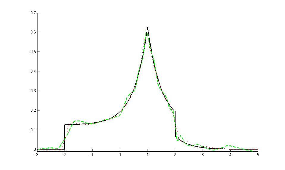
Figure 1: Estimators of the density $f$ (plain dark) for $T=10000$ and $\Delta=0.01$: the oracle (dotted red) and the estimator $\widehat{f}_{T,\Delta}$ (dashed green).

We approximate the $L_{2}$ errors by Monte Carlo. For that we compute $M=1000$ times each estimator (for $T=10000$ and $\Delta=0.01$) and approximate the $L_{2}$ loss by

$$\frac{1}{M}\sum_{i=1}^{M}\Big{(}\sum_{p=0}^{2000}\big{(}\widehat{f}(-10+0.01p)-f(-10+0.01p)\big{)}^{2}\times 0.01\Big{)}.$$

For each Monte Carlo iteration the estimators are evaluated on the same trajectory. The results are reproduced in the following table.

Estimator	Oracle	$\widehat{f}_{T,\Delta}$
$L_{2}$ error ($\times 10^{-4}$)	0.1916	0.2040
Standard deviation ($\times 10^{-5}$)	0.4519	0.4605

4.2 Illustration in the slow microscopic case

We now study the behaviour of the estimator corrected at order $K$ for different values of $K$. We choose $T=10000$ and $\Delta=0.1$. In that case $T\Delta^{2}$ is large but $T\Delta^{4}$ is 1. According to Theorem 2 we should observe that the estimator corrected at order 2, behaves as the oracle. Figure 2 represents the estimators $\widehat{f}^{K}_{T,\Delta}$ defined in Definition 2 for $K\in\{0,1,2,3\}$ and the oracle. The estimators are evaluated on the same trajectory. They all manage to reproduce the shape of the density $f$, and graphically apart from the estimator corrected at order 0 they are difficult to distinguish.

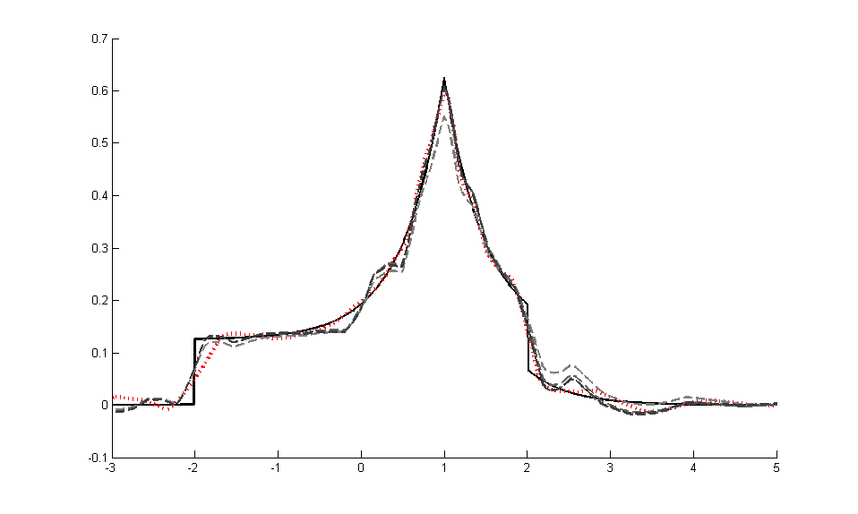
Figure 2: Estimators of the density $f$ (plain dark) for $T=10000$ and $\Delta=0.1$: the oracle (dotted red) and the estimator $\widehat{f}^{K}_{T,\Delta}$ for $K=0,1,2,3$ (dashed light to dark grey).

We compare their $L_{2}$ losses in the following tabular.

Estimator	Oracle	$K=0$	$K=1$	$K=2$	$K=3$
$L_{2}$ error ($\times 10^{-4}$)	0.1896	0.5176	0.3037	0.2959	0.2946
Standard deviation ($\times 10^{-5}$)	0.4348	0.7800	0.7533	0.7462	0.7466

This confirms that there is an actual gain in considering the estimator corrected at order 1 instead of the uncorrected one. In the following table we estimate the $\big{(}p_{m}(\Delta)\big{)}$ defined in Proposition 1.

Estimated quantity	$\widehat{p_{1}}$	$\widehat{p_{2}}$	$\widehat{p_{3}}$
Estimation	0.8527	0.1327	0.0135
Standard deviation ($\times 10^{-3}$)	0.9185	0.7388	0.1597

It turns out that making no correction is equivalent to estimate a density on a data set where $15\%$ of the observations are realisations of a law which is not target. This explains why it is relevant to take them into account when estimating $f$. Considering more than 1 or 2 corrections is unnecessary as the $L_{2}$ losses get stable afterwards. The $L_{2}$ loss of the oracle is strictly lower than the loss of the estimator corrected at order $K$, even for large $K$. That difference is explained by the fact that to estimate the $m$th convolution power we do not use $N_{T}$ data points but $N_{T,m}=\lfloor N_{T}/m\rfloor$. Therefore we do not loose in terms of rate of convergence, but we surely deteriorate the constants in comparison with the oracle.

5 Discussion and Conclusion

Attainable rates.

Without loss of generality, assuming $T$ is an integer if we observe $T$ independent realisations of the density $f$, it is possible to achieve the minimax rates of convergence $T^{-\alpha(s,\pi,p)}$ (see for instance Donoho et al. [10]). When the process $X$ is continuously observed over $[0,T]$, we have $R_{T}$ independent and identically distributed realisations of $f$. Moreover for $T$ large enough, the elementary renewal theorem guarantees that $R_{T}$ is of the order of $T$ (see for instance Lindvall [19]). It follows that the estimators of $f$ given in Sections 2 and 3 enables to attain the minimax rates of convergence of an experiment where $X$ is continuously observed.

Comparison with a previous work.

The results of this paper are the generalisation to the renewal reward case of Duval [11]; a compound Poisson process is a particular renewal reward process and Theorems 1 and 2 enable to recover the results of [11]. However in this paper we do not have an explicit formula for the estimator corrected at order $K$ but only a construction method. In the Poisson case it is much more simpler to apply the results of [11].

Extension to the case where $\Delta$ is fixed.

We established Theorem 2 for $\Delta_{T}$ vanishing to 0. Since the approximation of the inverse depends only the fact that $\mathbf{H}_{\Delta,f}$ is a contraction, the method remains valid for $\Delta$’s such that $\mathfrak{K}(\Delta)$ defined in (18) is strictly lower than 1. Which means that we can expand the results to cases where $\Delta$ does not go to 0 but satisfies $\mathfrak{K}(\Delta)<1.$ The value of the maximum value $\Delta_{1}$ satisfying the former inequality depends on $\tau(0)$ and $\mathfrak{O}$ but is not only determined by (18). Another hidden condition on $\Delta$ have to be satisfied for $\mathbf{H}_{\Delta,f}$ to send elements of $\mathcal{H}(s,{\pi},\mathfrak{O},\mathfrak{N})$ into itself. Then to find $\Delta_{1}$ one has to solve an optimisation program with constraints to find $\Delta_{1}$ and $\mathfrak{O}$ giving the maximum coverage for $\Delta$. To get an idea of the value of $\Delta_{1}$ we use the function NMaximize of Mathematica and find that one should take $\mathfrak{O}=1.645$ and $\Delta_{1}=0.071/\tau(0)>0,$ which is positive. The results of Theorem 2 should generalise in for all $\Delta_{T}\rightarrow\Delta_{\infty}$ such that $\Delta_{\infty}<\Delta_{1}$ and for $K\in\mathbb{N}$ the rate of convergence for the estimator corrected at order $K$ is bounded by

$$\max\big{\{}T^{-\alpha(s,p,\pi)},\Delta^{K+1}_{\infty}\big{\}}.$$

However to achieve suitable rates theoretically one should consider larger $K$, therefore the dependency in $K$ in the constants need to be handled carefully. In practice for $T=10000$ and $\Delta=0.1$ considering $K=2$ appears sufficient to have $T^{-\alpha(s,p,\pi)}$ predominant in front of $\Delta^{K+1}$.

Discussion on Assumptions 1 and 3.

In the present paper we made two simplifying assumptions on the interarrival density $\tau$. First we assume that $J_{1}$ was distributed according to $\tau_{0}$ to work with a process with stationary increments. In fact if $\tau$ has finite expectation this assumption is not necessary since asymptotically the process has stationary increments (see Lindvall [19]). The second assumption is that $\tau$ is described by a 1-dimensional parameter $\vartheta$. Generalising the result to a $d$-dimensional parameter should be possible at small cost, but removing all parametric assumption on $\tau$ would demand to solve a nonstandard nonparametric program for $\tau$ from the observations (2): observations (2) only give access to truncated values of realisations of $\tau$ spaced of more than $\Delta$. Then the problem of estimating $\tau$ from (2) should be considered separately.

Other generalisations.

We constructed in the microscopic regime an adaptive minimax estimator of the jump density of a renewal reward process. The methodology presented here should adapt to any process defined similarly to $X$ but whose counting process has stationary increments and manageable dependencies. We consider in the present paper a renewal counting measure since we are interested in expanding the methodology to other regimes of $\Delta$, namely when $\Delta=\Delta_{T}$ tends to a constant (intermediate regime) or to infinity (macroscopic regime). The macroscopic regime is of special interest since the observed process presents diffusive or anomalous asymptotic behaviour determined by the laws $f$ and $\tau$ (see for instance Meerschaert and Scheffler [21, 22] or Kotulski [18]) and many applications have a model based on a macroscopically observed renewal reward processes. For instance in physics where they are used to model particle motion (see Watkins and Credgington [30] or Cuppen et al. [8]), in biology to model the proliferation of tumor cells (see Fedotov and Iomin [12]) or lipid granule motion (see Jeon et al. [16]), they are also used to model records (see Sabhapandit [25]).

6 Proofs

In the sequel $\mathfrak{C}$ denotes a constant which may vary from line to line.

6.1 Proof of Theorem 1

Proof of part 1) of Theorem 1

To prove part 1) of Theorem 1 we apply the general results of Kerkyacharian and Picard [17]. For that we establish some technical lemmas.

Lemma 2.

If $f$ belongs to $\mathcal{F}(s,{\pi},\mathfrak{M})$ then for $m\geq 1$, $\mathbf{P}_{\Delta}[f]^{\star m}$ also belongs to $\mathcal{F}(s,{\pi},\mathfrak{M})$.

To prove Theorem 1, we use Lemma 2 for $m=1$ only, but we take some advance on the proof of Theorem 2.

Proof of Lemma 2.

It is straightforward to derive $\big{\|}\mathbf{P}_{\Delta}[f]^{\star m}\big{\|}_{L_{1}(\mathbb{R})}=1$. The remainder of the proof is a consequence of the following result: Let $f\in{\mathcal{B}^{s}_{{\pi}\infty}(\mathcal{D})}$ and $g\in L_{1}$ we have

$$\|f\star g\|_{{\mathcal{B}^{s}_{{\pi}\infty}(\mathcal{D})}}\leq\|f\|_{{\mathcal{B}^{s}_{{\pi}\infty}(\mathcal{D})}}\|g\|_{L_{1}(\mathbb{R})}.$$ (25)

To prove (25) we use the definition of the Besov norm (8); the result is a consequence of Young’s inequality and elementary properties of the convolution product. First Young’s inequality gives

$$\|f_{1}\star f_{2}\|_{L_{\pi}(\mathbb{R})}\leq\|f_{1}\|_{L_{\pi}(\mathbb{R})}\|f_{2}\|_{L_{1}(\mathbb{R})}.$$ (26)

Then the differentiation property of the convolution product leads for $n\geq 1$ to

$$\Big{\|}\frac{d^{n}}{dx^{n}}(f_{1}\star f_{2})\Big{\|}_{L_{\pi}(\mathcal{D})}=\Big{\|}\Big{(}\frac{d^{n}}{dx^{n}}f_{1}\Big{)}\star f_{2}\Big{\|}_{L_{\pi}(\mathbb{R})}\leq\Big{\|}\frac{d^{n}}{dx^{n}}f_{1}\Big{\|}_{L_{\pi}(\mathcal{D})}\|f_{2}\|_{L_{1}(\mathbb{R})}.$$ (27)

Finally translation invariance of the convolution product enables to get

$$\big{\|}\mathbf{D}^{h}\mathbf{D}^{h}[(f_{1}\star f_{2})^{(n)}]\big{\|}_{L_{\pi}(\mathcal{D})} =\big{\|}(\mathbf{D}^{h}\mathbf{D}^{h}[f_{1}^{(n)}])\star f_{2}\big{\|}_{L_{\pi}(\mathcal{D})}$$

$$\leq\big{\|}\mathbf{D}^{h}\mathbf{D}^{h}[f_{1}^{(n)}]\big{\|}_{L_{\pi}(\mathcal{D})}\|f_{2}\|_{L_{1}(\mathbb{R})}.$$ (28)

Inequality (25) is then obtained by bounding $\|f\star g\|_{{\mathcal{B}^{s}_{{\pi}\infty}(\mathcal{D})}}$ using (26), (27) and (28). To complete the proof of Lemma 2, we apply $m-1$ times (25) which leads to

$$\forall m\in\mathbb{N}\setminus\{0\},\ \ \ \ \ \big{\|}\mathbf{P}_{\Delta}[f]^{\star m}\big{\|}_{{\mathcal{B}^{s}_{{\pi}\infty}(\mathcal{D})}}\leq\big{\|}\mathbf{P}_{\Delta}[f]\big{\|}_{{\mathcal{B}^{s}_{{\pi}\infty}(\mathcal{D})}}.$$

The triangle inequality gives $\|\mathbf{P}_{\Delta}[f]^{\star m}\|_{{\mathcal{B}^{s}_{{\pi}\infty}(\mathcal{D})}}\leq\|f\|_{{\mathcal{B}^{s}_{{\pi}\infty}(\mathcal{D})}}\leq\mathfrak{M}$ which concludes the proof. ∎

Lemma 3.

Let $2^{j}\leq T$, then for $p\geq 1$ we have

$$\mathbb{E}\big{[}\big{|}\widehat{\gamma}_{jk}-\gamma_{jk}\big{|}^{p}\big{]}\leq\mathfrak{C}_{p,\|g\|_{L_{p}(\mathbb{R})},\mathfrak{M}}T^{-p/2},$$

where $\widehat{\gamma}_{jk}$ is defined in (13) and

$$\gamma_{jk}=\int g_{jk}(y)\mathbf{P}_{\Delta}[f](y)dy.$$ (29)

Proof of Lemma 3.

The proof is obtained with Rosenthal’s inequality: let $p\geq 1$ and let $(Y_{1},\ldots,Y_{n})$ be independent random variables such that $\mathbb{E}[Y_{i}]=0$ and $\mathbb{E}\big{[}|Y_{i}|^{p}\big{]}<\infty$. Then there exists $\mathfrak{C}_{p}$ such that

$$\mathbb{E}\bigg{[}\Big{|}\sum_{i=1}^{n}Y_{i}\Big{|}^{p}\bigg{]}\leq\mathfrak{C}_{p}\bigg{\{}\sum_{i=1}^{n}\mathbb{E}\big{[}|Y_{i}|^{p}\big{]}+\Big{(}\sum_{i=1}^{n}\mathbb{E}\big{[}|Y_{i}|^{2}\big{]}\Big{)}^{p/2}\bigg{\}}.$$ (30)

According to Proposition 1 the $\big{(}\mathbf{D}^{\Delta_{T}}X_{i}\big{)}$ have distribution

$$f_{\mathbf{D}^{\Delta_{T}}(x)X_{1}}=p(\Delta_{T})\delta_{0}(x)+\big{(}1-p(\Delta_{T})\big{)}\mathbf{P}_{\Delta_{T}}[f](x),\ \ \ \ x\in\mathcal{D}$$

where $\delta_{0}$ is the Dirac delta function and $p(\Delta_{T})=\mathbb{P}(R_{\Delta_{T}}=0)$. We derive

$$\mathbb{E}\big{[}\widehat{\gamma}_{jk}\big{]} =\int g_{jk}(z)\mathds{1}_{\{z\neq 0\}}\frac{f_{\mathbf{D}^{\Delta_{T}}X_{1}}(z)}{1-p(\Delta_{T})}dz=\int g_{jk}(z)\mathbf{P}_{\Delta_{T}}[f](z)dz=\gamma_{jk}.$$

Then $\widehat{\gamma}_{jk}-\gamma_{jk}$ is a sum of centered and identically distributed random variables, define

$$Z_{i}=\frac{1}{1-p(\Delta_{T})}g_{jk}\big{(}\mathbf{D}^{\Delta_{T}}X_{i}\big{)}\mathds{1}_{\{\mathbf{D}^{\Delta_{T}}X_{i}\neq 0\}}.$$

Since $x$ is a renewal reward process, nonzero and nonconsecutive $Z_{i}$ are independent, then if we separate the sum in two sums of nonzero and nonconsecutive indices we can apply Rosenthal’s inequality for independent variables to each sum, it wont affect the rates but the constant will modified. For $p\geq 1$ we have by convex inequality

$$\mathbb{E}\big{[}\big{|}Z_{i}-\mathbb{E}[Z_{i}]\big{|}^{p}\big{]} \leq 2^{p}\mathbb{E}\big{[}\big{|}Z_{i}\big{|}^{p}\big{]}$$

$$\leq\frac{2^{p}2^{jp/2}}{\big{(}1-p(\Delta_{T})\big{)}^{p}}\int|g(2^{j}y-k)|^{p}\mathds{1}_{\{y\neq 0\}}f_{\mathbf{D}^{\Delta_{T}}}(y)dy$$

$$=\frac{2^{p}2^{j(p/2-1)}}{\big{(}1-p(\Delta_{T})\big{)}^{p-1}}\int|g(z)|^{p}\mathbf{P}_{\Delta_{T}}[f]\Big{(}\frac{z+k}{2^{j}}\Big{)}dz,$$

where we made the substitution $z=2^{j}y-k$. Lemma 2 and Sobolev embeddings (see [4, 10, 14])

$$\mathcal{B}^{s}_{{\pi}\infty}\hookrightarrow\mathcal{B}^{s^{\prime}}_{p\infty}\ \ \ \mbox{ and }\ \ \ \mathcal{B}^{s^{\prime}}_{{\pi}\infty}\hookrightarrow\mathcal{B}^{s}_{{\infty}\infty},$$ (31)

where $p>\pi$, $s\pi>1$ and $s^{\prime}=s-1/\pi+1/p$, give $\big{\|}\mathbf{P}_{\Delta_{T}}[f]\big{\|}_{\infty}\leq\mathfrak{M}$. It follows that

$$\mathbb{E}\big{[}\big{|}Z_{i}-\mathbb{E}[Z_{i}]\big{|}^{p}\big{]}\leq 2^{p}2^{j(p/2-1)}\|g\|_{L_{p}(\mathbb{R})}^{p}\mathfrak{M}/(1-p(\Delta_{T}))^{p-1}$$

and

$$\mathbb{E}\big{[}\big{|}Z_{i}-\mathbb{E}[Z_{i}]\big{|}^{2}\big{]}\leq\mathfrak{M}/(1-p(\Delta_{T}))$$

since $\|g\|_{L_{2}(\mathbb{R})}=1$. Rosenthal’s inequality (30) gives for $p\geq 1$

$$\mathbb{E}\big{[}\big{|}\widehat{\gamma}_{jk}-\gamma_{jk}\big{|}^{p}\big{]} \leq\mathfrak{C}_{p}\Big{\{}2^{p}\Big{(}\frac{2^{j}}{A_{T}}\Big{)}^{\frac{p}{2}-1}\|g\|_{L_{p}(\mathbb{R})}^{p}\mathfrak{M}+\mathfrak{M}^{p/2}\Big{\}}A_{T}^{-\frac{p}{2}},$$

where $A_{T}=\lfloor T\Delta_{T}^{-1}\rfloor(1-p(\Delta_{T}))$. To conclude we use that

$$1-p(\Delta_{T})=\mathbb{P}(J_{1}\geq\Delta_{T})=\frac{1}{\mu}\int_{0}^{\Delta_{T}}\big{(}1-F(u)\big{)}du,$$

since $J_{1}$ has distribution (1), and derive that there exists $\Delta_{1}>0$ such that $F(\Delta_{1})\leq\frac{1}{2}$ and for all $\Delta_{T}\leq\Delta_{1}$ we have

$$\frac{\Delta_{T}}{2\mu}\leq 1-p(\Delta_{T})\leq\frac{\Delta_{T}}{\mu}.$$ (32)

It follows that

$$\frac{T}{2\mu}\leq A_{T}\leq\frac{T}{\mu}$$

and then using $2^{j}\leq T$

$$\mathbb{E}\big{[}\big{|}\widehat{\gamma}_{jk}-\gamma_{jk}\big{|}^{p}\big{]} \leq\mathfrak{C}_{p,\|g\|_{L_{p}(\mathbb{R})},\mathfrak{M},\mu}T^{-p/2}.$$

The proof the complete.∎

Lemma 4.

Choose $j$ and $c$ such that

$$2^{j}T^{-1}\log(T^{1/2})\leq 1\mbox{ and }c^{2}\geq 32\mu\Big{(}\mathfrak{M}+\frac{c\|g\|_{\infty}}{6}\Big{)}.$$

For all $r\geq 1$, let $\kappa_{r}=cr$. We have

$$\mathbb{P}\Big{(}\big{|}\widehat{\gamma}_{jk}-\gamma_{jk}\big{|}\geq\frac{\kappa_{r}}{2}T^{-1/2}\sqrt{\log(T^{1/2})}\Big{)}\leq T^{-r/2},$$

where $\widehat{\gamma}_{jk}$ is defined in (13) and $\gamma_{jk}$ in (29).

Proof of Lemma 4.

The proof is obtained with Bernstein’s inequality. Consider $Y_{1},\ldots,Y_{n}$ independent random variables such that $|Y_{i}|\leq\mathfrak{A}$, $\mathbb{E}[Y_{i}]=0$ and $b_{n}^{2}=\sum_{i=1}^{n}\mathbb{E}[Y_{i}^{2}]$. Then for any $\lambda>0$,

$$\mathbb{P}\Big{(}\Big{|}\sum_{i=1}^{n}Y_{i}\Big{|}>\lambda\Big{)}\leq 2\exp\Big{(}-\frac{\lambda^{2}}{2(b_{n}^{2}+\frac{\lambda\mathfrak{A}}{3})}\Big{)}.$$ (33)

We keep notation $Z_{i}$ introduced in the proof of Lemma 3, $\widehat{\gamma}_{jk}-\gamma_{jk}$ is a sum of centered and identically distributed random variables bounded by $2^{j/2}\|g\|_{\infty}/(1-p(\Delta_{T}))$ which verify

$$\mathbb{E}\big{[}\big{|}Z_{i}-\mathbb{E}[Z_{i}]\big{|}^{2}\big{]}\leq\mathfrak{M}/(1-p(\Delta_{T})).$$

After separating the sum to get two sums of nonzero and nonconsecutive indices we apply Bernstein’s inequality (33) for independent variables to each sum, which modify the constants. It follows that

$$\mathbb{P}\Big{(}|\widehat{\gamma}_{jk}-\gamma_{jk}| \geq\frac{\kappa_{r}}{2}T^{-1/2}\sqrt{\log(T^{1/2})}\Big{)}$$

$$\leq 2\exp\Bigg{(}-\frac{\kappa_{r}^{2}T^{-1}\log(T^{1/2})\lfloor T\Delta_{T}^{-1}\rfloor\big{(}1-p(\Delta_{T})\big{)}}{16\Big{(}\mathfrak{M}+\frac{\kappa_{r}T^{-1/2}\sqrt{\log(T^{1/2})}2^{j/2}\|g\|_{\infty}}{6}\Big{)}}\Bigg{)}.$$

Using that $2^{j}T^{-1}\log(T^{1/2})\leq 1$ and (32) which gives

$$T^{-1}\lfloor T\Delta_{T}^{-1}\rfloor(1-p(\Delta_{T}))\geq\frac{1}{2\mu},$$

we have

$$\mathbb{P}\Big{(}|\widehat{\gamma}_{jk}-\gamma_{jk}| \geq\frac{\kappa_{r}}{2}T^{-1/2}\sqrt{\log(T^{1/2})}\Big{)}$$

$$\leq 2\exp\bigg{(}-\frac{c^{2}r}{32\mu\big{(}\mathfrak{M}+\frac{\kappa_{r}\|g\|_{\infty}}{6}\big{)}}r\log(T^{1/2})\bigg{)}\leq T^{-r/2},$$

since $c^{2}\geq 32\mu\big{(}\mathfrak{M}+\frac{c\left\|g\right\|_{\infty}}{6}\big{)}.$ The proof is complete.∎

Proof of of part 1) of Theorem 1.

It is a consequence of Lemma 2, 3, 4 and of the general theory of wavelet threshold estimators of Kerkyacharian and Picard [17]. It suffices to have conditions (5.1) and (5.2) of Theorem 5.1 of [17], which are satisfied –Lemma 3 and 4– with $c(T)=T^{-1/2}$ and $\Lambda_{n}=c(T)^{-1}$ (with the notation of [17]). We can now apply Theorem 5.1, its Corollary 5.1 and Theorem 6.1 of [17] to obtain the result. ∎

Completion of the proof of Theorem 1

To prove part 2) of Theorem 1 we decompose the $L_{p}$ loss as follows

$$\big{(}\mathbb{E}\big{[}\|\widehat{f}_{T,\Delta_{T}}- f\|_{L_{p}(\mathcal{D})}^{p}\big{]}\big{)}^{1/p}$$

$$\leq\big{(}\mathbb{E}\big{[}\big{\|}\widehat{f}_{T,\Delta_{T}}-\mathbf{P}_{\Delta_{T}}[f]\|_{L_{p}(\mathcal{D})}^{p}\big{]}\big{)}^{1/p}+\big{\|}\mathbf{P}_{\Delta_{T}}[f]-f\big{\|}_{L_{p}(\mathcal{D})}.$$

An upper bound for the first term is given by part 1) of Theorem 1

$$\big{(}\mathbb{E}\big{[}\big{\|}\widehat{f}_{T,\Delta_{T}}-\mathbf{P}_{\Delta_{T}}[f]\|_{L_{p}(\mathcal{D})}^{p}\big{]}\big{)}^{1/p} \leq\mathfrak{C}T^{-\alpha(s,p,\pi)},$$ (34)

where $\mathfrak{C}$ continuously depends on $\mu$, and on $s,\pi,p,\mathfrak{M},\phi,\psi$ and $\mu$. Since

$$\mathbf{P}_{\Delta_{T}}[f]-f=-(1-p_{1}(\Delta_{T}))f+\sum_{m=2}^{\infty}p_{m}(\Delta_{T})\mathbf{P}_{\Delta_{T}}[f]^{\star m}$$

Lemma 1, Young’s inequality, which gives $\|\mathbf{P}_{\Delta_{T}}[f]^{\star m}\|_{L_{p}(\mathcal{D})}\leq\|f\|_{L_{p}(\mathcal{D})}$ and Sobolev embeddings (31), which give $\|f\|_{L_{p}(\mathcal{D})}\leq\mathfrak{M}$, enable to get the bound

$$\big{\|}\mathbf{P}_{\Delta_{T}}[f]-f\big{\|}_{L_{p}(\mathcal{D})} \leq 2\tau(0)\Delta_{T}+2\mathfrak{M}\sum_{m=2}^{\infty}\frac{\big{(}2\tau(0)\Delta_{T}\big{)}^{m-1}}{m!}\leq\mathfrak{C}\Delta_{T},$$ (35)

where $\mathfrak{C}$ continuously depends on $\tau(0)$ and $\mathfrak{M}$. We finish the proof noticing that (34) is predominant in front of (35) since $\alpha(s,p,\pi)\leq 1/2$ and $T\Delta_{T}^{2}=O(1)$. Finally we take the supremum in $\mu$ and $\tau(0)$ over any compact of $(0,\infty)$ to render the constant independent of the unknown interarrival law $\tau$. The proof is now complete.

6.2 Proof of Proposition 2

First we prove part 1) of Proposition 2. The set $\mathcal{H}(s,{\pi},\mathfrak{O},\mathfrak{N})$ is a subset of

$$\big{(}\mathcal{B}^{s}_{{\pi}\infty}(\mathcal{D}),\|.\|_{\mathcal{B}^{s}_{{\pi}\infty}(\mathcal{D})}\big{)}$$

which is a Banach space. We show that $\mathcal{H}(s,{\pi},\mathfrak{O},\mathfrak{N})$ is complete since it is a closed subset of a Banach space. For that we establish the following assertions; for all sequence $h_{n}\in\mathcal{H}(s,{\pi},\mathfrak{O},\mathfrak{N})$ such that there exists $h$ with

$$\|h_{n}-h\|_{\mathcal{B}^{s}_{{\pi}\infty}(\mathcal{D})}\rightarrow 0,\ \ \ \mbox{ as }n\rightarrow\infty,$$

we have $h\in\mathcal{H}(s,{\pi},\mathfrak{O},\mathfrak{N})$ i.e. $\|h\|_{\mathcal{B}^{s}_{{\pi}\infty}(\mathcal{D})}\leq\mathfrak{N}$ and $\|h\|_{L_{1}(\mathcal{D})}\leq\mathfrak{O}$. The first inequality is immediate. The second one is a consequence of the compactness of $\mathcal{D}$. Indeed

$$\|h_{n}-h\|_{\mathcal{B}^{s}_{{\pi}\infty}(\mathcal{D})}\rightarrow 0,\ \ \ \mbox{ as }n\rightarrow\infty,$$

we have by definition of the Besov norm (8) that

$$\|h_{n}-h\|_{L_{\pi}(\mathcal{D})}\rightarrow 0,\ \ \ \mbox{ as }n\rightarrow\infty.$$

Since $\mathcal{D}$ is compact and $\pi\geq 1$ we derive from Hölder’s inequality that

$$\|h_{n}-h\|_{L_{1}(\mathcal{D})}\rightarrow 0,\ \ \ \mbox{ as }n\rightarrow\infty$$

and then $\|h\|_{L_{1}(\mathcal{D})}\leq\mathfrak{O}$ follows. The proof of part 1) of Proposition 2 is now complete.

To prove part 2) of Proposition 2 we show that $\mathbf{H}_{\Delta,f}$ sends elements of $\mathcal{H}(s,{\pi},\mathfrak{O},\mathfrak{N})$ into $\mathcal{H}(s,{\pi},\mathfrak{O},\mathfrak{N})$ and that it is a contraction. We start with the first assertion, the triangular inequality gives for $h\in\mathcal{H}(s,{\pi},\mathfrak{O},\mathfrak{N})$

$$\big{\|}\mathbf{H}_{\Delta,f}[h]\big{\|}_{L_{1}(\mathcal{D})} \leq\big{\|}\mathbf{P}_{\Delta}[f]\big{\|}_{L_{1}(\mathcal{D})}+\big{(}1-p_{1}(\Delta)\big{)}\|h\|_{1}+\sum_{m=2}^{\infty}p_{m}(\Delta)\|h^{\star m}\|_{L_{1}(\mathcal{D})},$$

where $\big{\|}\mathbf{P}_{\Delta}[f]\big{\|}_{L_{1}(\mathcal{D})}\leq\big{\|}\mathbf{P}_{\Delta}[f]\big{\|}_{L_{1}(\mathbb{R})}=1$. Immediate induction on Young’s inequality leads to

$$\|h^{\star m}\|_{L_{1}(\mathcal{D})}\leq\|h\|_{L_{1}(\mathcal{D})}^{m}\leq\mathfrak{O}^{m}$$

since $h\in\mathcal{H}(s,{\pi},\mathfrak{O},\mathfrak{N})$ and with Lemma 1 we get

$$\big{\|}\mathbf{H}_{\Delta,f}[h]\big{\|}_{1} \leq 1+2\mathfrak{O}\tau(0)\Delta+\frac{1}{\tau(0)\Delta}(e^{2\mathfrak{O}\tau(0)\Delta}-1-2\mathfrak{O}\tau(0)\Delta)\leq\mathfrak{O}$$

for $\Delta$ small enough since $\mathfrak{O}>1$. Similar computations and (25) give

$$\big{\|}\mathbf{H}_{\Delta,f}[h]\big{\|}_{\mathcal{B}^{s}_{{\pi}\infty}(\mathcal{D})}\leq \big{\|}\mathbf{P}_{\Delta}[f]\big{\|}_{\mathcal{B}^{s}_{{\pi}\infty}(\mathcal{D})}+\big{(}1-p_{1}(\Delta)\big{)}\|h\|_{\mathcal{B}^{s}_{{\pi}\infty}(\mathcal{D})}$$

$$+\sum_{m=2}^{\infty}p_{m}(\Delta)\|h^{\star m}\|_{\mathcal{B}^{s}_{{\pi}\infty}(\mathcal{D})}$$

$$\leq \mathfrak{M}+2\tau(0)\Delta\mathfrak{N}+\frac{\mathfrak{N}}{\tau(0)\Delta\mathfrak{O}}(e^{2\mathfrak{O}\tau(0)\Delta}-1-2\mathfrak{O}\tau(0)\Delta)\leq\mathfrak{N},$$

for $\Delta$ small enough since $\mathfrak{M}<\mathfrak{N}$. Then if $h$ is in $\mathcal{H}(s,{\pi},\mathfrak{O},\mathfrak{N})$, $\mathbf{H}_{\Delta,f}$ belongs to $\mathcal{H}(s,{\pi},\mathfrak{O},\mathfrak{N})$.

For the contraction property, we have for all $h_{1},h_{2}\in\mathcal{H}(s,{\pi},\mathfrak{O},\mathfrak{N})$

$$\mathbf{H}_{\Delta,f}[h_{1}]-\mathbf{H}_{\Delta,f}[h_{2}]= (1-p_{1}(\Delta))(h_{1}-h_{2})$$

$$-(h_{1}-h_{2})\star\sum_{m=2}^{\infty}p_{m}(\Delta)\sum_{q=0}^{m-1}h_{1}^{\star q}\star h_{2}^{\star m-1-q}$$ (36)

Lemma 1 gives

$$0\leq 1-p_{1}(\Delta)\leq 2\tau(0)\Delta,$$ (37)

and with Young’s inequality and since $h_{1}$ and $h_{2}$ belong to $\mathcal{H}(s,{\pi},\mathfrak{O},\mathfrak{N})$ we get

$$\Big{\|}\sum_{m=2}^{\infty}p_{m}(\Delta)\sum_{q=0}^{m-1}h_{1}^{\star q}\star h_{2}^{\star m-1-q}\Big{\|}_{L_{1}(\mathcal{D})} \leq 2\mathfrak{O}\big{(}e^{2\tau(0)\mathfrak{O}\Delta}-1\big{)}$$ (38)

for $\Delta$ small enough. Finally injecting (37) and (38) into (36) leads to the contraction property for all $h_{1},h_{2}\in\mathcal{H}(s,{\pi},\mathfrak{O},\mathfrak{N})$

$$\big{\|}\mathbf{H}_{\Delta,f}[h_{1}]-\mathbf{H}_{\Delta,f}[h_{2}]\big{\|}_{\mathcal{B}^{s}_{{\pi}\infty}(\mathcal{D})}\leq\big{(}2\tau(0)\Delta+2\mathfrak{O}\big{(}e^{2\tau(0)\mathfrak{O}\Delta}-1\big{)}\big{)}\|h_{1}-h_{2}\|_{\mathcal{B}^{s}_{{\pi}\infty}(\mathcal{D})},$$

which concludes the proof.

6.3 Proof of Theorem 2

Preliminary

The estimators of the convolution powers of $\mathbf{P}_{\Delta}[f]$ depend on $N_{T}$ which is random and depends on the $\mathbf{D}^{\Delta}_{m}X_{i}$.

Lemma 5.

Work under Assumption 4 and let $p(\Delta)=\mathbb{P}(R_{\Delta}\neq 0)$ and $\Delta_{1}$ be such that $\int_{0}^{\Delta_{1}}\tau(x)dx\leq\frac{1}{2}.$ Then for all $\lambda>0$ and $\Delta\leq\Delta_{1}$ we have

$$\mathbb{P}\Big{(}\Big{|}\frac{N_{T}}{\lfloor T\Delta^{-1}\rfloor}-p(\Delta)\Big{|}>\lambda\Delta\Big{)}\leq\exp\Big{(}-\mathfrak{C}\sqrt{T}\Delta\Big{)},$$

where $\mathfrak{C}$ depends on $\mathfrak{A},\mathfrak{a},\mathfrak{g},\mu,\lambda$.

Proof of Lemma 5.

We have

$$\frac{N_{T}}{\lfloor T\Delta^{-1}\rfloor}-p(\Delta)=\frac{1}{\lfloor T\Delta^{-1}\rfloor}\sum_{i=1}^{\lfloor T\Delta^{-1}\rfloor}Y_{i},$$

where

$$Y_{i}=\mathds{1}_{\{\mathbf{D}^{\Delta}X_{i}\neq 0\}}-p(\Delta),\ \ \ \ i=1,\ldots,\lfloor T\Delta^{-1}\rfloor$$

are centered random variables, bounded by $M=1-p(\Delta)$ and such that

$$\mathbb{E}[Y_{i}^{2}]\leq p(\Delta).$$

To show the result, we apply Theorem 4.5 of Dedecker et. al. [9] which is a Bernstein-type inequality for dependent data. We have to verify conditions (4.4.16) and (4.4.17) of Theorem 4.5 of [9]. With their notation, condition (4.4.16) ensures that for all $u$-tuples $(s_{1},\ldots,s_{u})$ and all $v$-tuples $(t_{1},\ldots,t_{v})$ such that

$$1\leq s_{1}\leq\ldots\leq s_{u}\leq t_{1}\leq\ldots\leq t_{v}\leq\lfloor T\Delta^{-1}\rfloor$$

we have

$$\big{|}Cov(Y_{s_{1}}\ldots Y_{s_{u}},Y_{t_{1}}\ldots Y_{t_{v}})\big{|}\leq K^{2}M^{u+v-2}uv\rho(t_{1}-s_{u}),$$

for some positive constant $K$ and a nonincreasing function $\rho$ satisfying (4.4.17) namely

$$\sum_{s=0}^{\infty}(s+1)^{k}\rho(s)\leq L_{1}L_{2}^{k}(k!)^{\nu},\ \ \ \forall k\geq 0,$$

where $L_{1}$, $L_{2}$ and $\nu$ are positive constants.

Since $X$ is a renewal process, $Y_{s_{1}}\ldots Y_{s_{u}}$ and $Y_{t_{1}}\ldots Y_{t_{v}}$ are independent if there exists $r$ such that $s_{u}<r<t_{1}$ and $Y_{r}=1-p(\Delta)$ i.e there is a jump between $Y_{s_{u}}$ and $Y_{t_{1}}$. For the covariance to be nonzero it is necessary that no jump occurred between $s_{u}\Delta$ and $(t_{1}-1)\Delta$. Let $s=t_{1}-s_{u}-1$ using that $R$ is stationary we get an upper bound for $\rho$

$$\rho(t_{1}-s_{u})\leq\mathbb{P}\big{(}R_{(t_{1}-1)\Delta}-R_{s_{u}\Delta}=0\big{)}=\mathbb{P}\big{(}R_{s\Delta}=0\big{)}=\int_{s\Delta}^{\infty}\tau_{0}(x)dx$$ (39)

which decreases with $s$. Moreover since the $Y_{i}$ are centered and bounded by $M\leq 1$ we have by Cauchy-Schwarz and $\mathbb{E}[Y_{i}^{2}]\leq p(\Delta)$

$$\big{|}Cov(Y_{s_{1}}\ldots Y_{s_{u}},Y_{t_{1}}\ldots Y_{t_{v}})\big{|} \leq\big{|}Cov(Y_{s_{1}},Y_{t_{v}})\big{|}\leq\sqrt{\mathbb{E}\big{[}Y_{s_{1}}^{2}\big{]}\mathbb{E}\big{[}Y_{t_{v}}^{2}\big{]}}\leq p(\Delta).$$

We deduce that condition (4.4.16) is fulfilled with $K=p(\Delta)^{1/2}$ and the nonincreasing sequence $\rho$.

Next we show that $\rho$ satisfies (4.4.17), using Assumption 4 and (39) we get for $s\geq 1$

$$\rho(s) \leq\frac{1}{\mu}\int_{s\Delta_{T}}^{\infty}\big{(}1-\int_{0}^{x}\tau(t)dt\big{)}dx\leq\mathfrak{C}\exp\big{(}-\mathfrak{a}(s\Delta)^{\mathfrak{g^{\prime}}}\big{)},$$

where $\mathfrak{g}<\mathfrak{g^{\prime}}$ and $\mathfrak{C}$ depends on $\mathfrak{A},\mathfrak{a},\mu,\mathfrak{g}$. Which leads to for $k\geq 0$

$$\sum_{s=1}^{\infty}s^{k}\rho(s) \leq\sum_{s=1}^{1/\Delta}s^{k}+\mathfrak{C}\sum_{s=1/\Delta}^{\infty}s^{k}\exp\big{(}-\mathfrak{a}(s\Delta)^{\mathfrak{g^{\prime}}}\big{)}$$

$$\leq\Delta^{-(k+1)}+\mathfrak{C}\Delta^{-k}\sum_{s^{\prime}=1}^{\infty}s^{\prime k}\exp\big{(}-\mathfrak{a}(s^{\prime})^{\mathfrak{g^{\prime}}}\big{)}$$

$$\leq\mathfrak{C}\Delta^{-(k+1)}$$ (40)

where $\mathfrak{C}$ depends on $\mathfrak{A},\mathfrak{a},\mathfrak{g},\mu$, condition (4.4.17) follows with $L_{1}=\mathfrak{C}\Delta^{-1}$, $L_{2}=\Delta^{-1}$ and $\nu=0$.

We can now apply Theorem 4.5 which gives for all $\lambda>0$

$$\mathbb{P}\Big{(}\Big{|} \frac{N_{T}}{\lfloor T\Delta^{-1}\rfloor}-p(\Delta)\Big{|}>\lambda\Delta\Big{)}$$

$$\leq 2\exp\bigg{(}-\frac{\lfloor T\Delta^{-1}\rfloor^{2}\Delta^{2}\lambda^{2}}{2\big{(}\lfloor T\Delta^{-1}\rfloor p(\Delta)+(\lfloor T\Delta^{-1}\rfloor\Delta\lambda)^{3/2}\sqrt{2^{5}\Delta^{-2}}\big{)}}\bigg{)}.$$

Using (32) we derive for $\Delta\leq\Delta_{1}$

$$\mathbb{P}\Big{(}\Big{|}\frac{N_{T}}{\lfloor T\Delta^{-1}\rfloor}-p(\Delta)\Big{|}>\lambda\Delta\Big{)} \leq\exp\Big{(}-\mathfrak{C}\sqrt{T}\Delta\Big{)},$$

where $\mathfrak{C}$ depends on $\lambda,\mathfrak{A},\mathfrak{a},\mathfrak{g},\mu$. The proof is now complete. ∎

Proof of part 1) of Theorem 2

As for the proof of part 1) of Theorem 1 we apply the general results of Kerkyacharian and Picard [17] and first establish some technical lemmas.

Lemma 6.

Let $2^{j}\leq T$, then for $p\geq 1$ we have for all $m\geq 1$

$$\mathbb{E}\big{[}\big{|}\widehat{\gamma}_{jk}^{(m)}-\gamma_{jk}^{(m)}\big{|}^{p}\big{]}\leq\mathfrak{C}_{p,m,\|g\|_{L_{p}(\mathbb{R})},\mathfrak{M},\mu,\tau}T^{-p/2},$$

where $\widehat{\gamma}_{jk}^{(m)}$ is defined in (22) and

$$\gamma_{jk}^{(m)}=\int g_{jk}(y)\mathbf{P}_{\Delta}[f]^{\star m}(y)dy.$$ (41)

Proof of Lemma 6.

For $m\geq 1$, $\widehat{\gamma}_{jk}^{(m)}-\gamma_{jk}^{(m)}$ is the sum of $\lfloor N_{T}/m\rfloor$ identically distributed random variables, where $N_{T}$ is random. First we replace $N_{T}$ by its deterministic asymptotic limit using the following decomposition

$$\mathbb{E}\big{[}\big{|}\widehat{\gamma}_{jk}^{(m)}-\gamma_{jk}^{(m)}\big{|}^{p}\big{]}= \mathbb{E}\big{[}\big{|}\widehat{\gamma}_{jk}^{(m)}-\gamma_{jk}^{(m)}\big{|}^{p}\mathds{1}_{\big{\{}\big{|}\frac{N_{T}}{\lfloor T\Delta_{T}^{-1}\rfloor}-p(\Delta_{T})\big{|}\geq\lambda\big{\}}}\big{]}$$

$$+\mathbb{E}\big{[}\big{|}\widehat{\gamma}_{jk}^{(m)}-\gamma_{jk}^{(m)}\big{|}^{p}\mathds{1}_{\big{\{}|\frac{N_{T}}{\lfloor T\Delta_{T}^{-1}\rfloor}-p(\Delta_{T})\big{|}<\lambda\big{\}}}\big{]}.$$

Take $\lambda=1/4\mu$ and denote $n_{m}=\big{\lfloor}T/m\mu\big{\rfloor}$ and $n^{\prime}_{m}=\big{\lfloor}T/(4m\mu)\big{\rfloor}$, we have with that (32) that

$$\mathbb{E}\big{[}\big{|}\widehat{\gamma}_{jk}^{(m)}-\gamma_{jk}^{(m)}\big{|}^{p}\big{]}\leq 2^{jp/2}\|g\|_{\infty}\mathbb{P}\Big{(}\Big{|}\frac{N_{T}}{\lfloor T\Delta_{T}^{-1}\rfloor}-p(\Delta_{T})\Big{|}\geq\frac{\Delta_{T}}{4\mu}\Big{)}$$

$$+\mathbb{E}\Big{[}\Big{|}\frac{1}{n^{\prime}_{m}}\sum_{i=1}^{n_{m}}\big{(}\mathbf{D}^{\Delta}_{m}X_{S_{i}}-\mathbb{E}\big{[}\mathbf{D}^{\Delta}_{m}X_{S_{i}}\big{]}\big{)}\Big{|}^{p}\Big{]}.$$

For the first term of the right hand part, $T\Delta_{T}=O(T^{\delta})$, Lemma 5 and $2^{j}\leq T$ leads to

$$\mathbb{P}\Big{(}\big{|}\frac{N_{T}}{\lfloor T\Delta_{T}^{-1}\rfloor}-p(\Delta_{T})\big{|}\geq\frac{\Delta_{T}}{4\mu}\Big{)} \leq\mathfrak{C}T^{p/2}\exp\Big{(}-\mathfrak{C}T^{\delta}\Big{)}\leq\mathfrak{C}\exp(-T^{\delta^{\prime}_{p}}),$$ (42)

for some $\delta^{\prime}_{p}<\delta$ and where $\mathfrak{C}$ depends on $p,\|g\|_{\infty},\mathfrak{A},\mathfrak{a},\mu$. For the second term we apply Rosenthal’s inequality (30). Since $X$ is a renewal process the variables $\big{(}\mathbf{D}^{\Delta}_{m}X_{S_{2i}}\big{)}_{i}$ are independent but dependent of the variables $\big{(}\mathbf{D}^{\Delta}_{m}X_{S_{2i+1}}\big{)}_{i}$ which are independent. It ensures that the variables $\big{(}\mathbf{D}^{\Delta}_{m}X_{S_{i}}\big{)}$ are distributed according to $\mathbf{P}_{\Delta_{T}}[f]^{\star m}$. Moreover if we separate the sum $\widehat{\gamma}_{jk}^{(m)}-\gamma_{jk}^{(m)}$ between odd and even indices we can apply Rosenthal’s inequality for independent variables to each sum. For $p\geq 1$ we have by convex inequality

$$\mathbb{E}\big{[}\big{|}g_{jk}(\mathbf{D}^{\Delta}_{m}X_{S_{i}})-\gamma_{jk}\big{|}^{p}\big{]} \leq 2^{p}\mathbb{E}\big{[}\big{|}g_{jk}(\mathbf{D}^{\Delta}_{m}X_{S_{i}})\big{|}^{p}\big{]}$$

$$\leq 2^{p}2^{jp/2}\int|g(2^{j}y-k)|^{p}\mathbf{P}_{\Delta_{T}}[f]^{\star m}(y)dy$$

$$\leq 2^{p}2^{j(p/2-1)}\int|g(z)|^{p}\mathbf{P}_{\Delta_{T}}[f]^{\star m}\Big{(}\frac{z+k}{2^{j}}\Big{)}dz,$$

where we made the substitution $z=2^{j}y-k$. Lemma 2 and Sobolev embeddings (31) give $\big{\|}\mathbf{P}_{\Delta_{T}}[f]^{\star m}\big{\|}_{\infty}\leq\mathfrak{M}$. It follows that

$$\mathbb{E}\big{[}\big{|}g_{jk}(\mathbf{D}^{\Delta}_{m}X_{S_{i}})-\gamma_{jk}\big{|}^{p}\big{]}\leq 2^{p}2^{j(p/2-1)}\|g\|_{L_{p}(\mathbb{R})}^{p}\mathfrak{M}$$

and

$$\mathbb{E}\big{[}\big{|}g_{jk}(\mathbf{D}^{\Delta}_{m}X_{S_{i}})-\gamma_{jk}\big{|}^{2}\big{]}\leq\mathfrak{M}$$

since $\|g\|_{L_{2}(\mathbb{R})}=1$. We derive for $p\geq 1$

$$\mathbb{E}\Big{[}\Big{|}\frac{1}{n^{\prime}_{m}}\sum_{i=1}^{n_{m}} \big{(}\mathbf{D}^{\Delta}_{m}X_{S_{i}}-\mathbb{E}\big{[}\mathbf{D}^{\Delta}_{m}X_{S_{i}}\big{]}\big{)}\Big{|}^{p}\Big{]}$$

$$\leq\mathfrak{C}_{p}\Big{\{}2^{p}\Big{(}\frac{2^{j}}{n_{m}}\Big{)}^{\frac{p}{2}-1}\|g\|_{L_{p}(\mathbb{R})}^{p}\mathfrak{M}+\mathfrak{M}^{p/2}\Big{\}}{n_{m}^{\prime}}^{-p/2}$$

$$\leq\mathfrak{C}_{p,m,\|g\|_{L_{p}(\mathbb{R})},\mathfrak{M},\mu}T^{-p/2}.$$ (43)

It follows from (42) and (43) that

$$\mathbb{E}\big{[}\big{|}\widehat{\gamma}_{jk}^{(m)}-\gamma_{jk}^{(m)}\big{|}^{p}\big{]}\leq \mathfrak{C}\exp(-T^{\delta^{\prime}_{p}})+\mathfrak{C}T^{-\frac{p}{2}}\leq\mathfrak{C}T^{-\frac{p}{2}},$$

since the first term is negligible in front of the second as $\delta^{\prime}>0$ where $\mathfrak{C}$ depends on $p,m,\|g\|_{L_{p}(\mathbb{R})},\|g\|_{\infty},\mathfrak{A},\mathfrak{a},\mathfrak{M},\mu$. It concludes the proof. ∎

Lemma 7.

Choose $j$ and $c$ such that

$$2^{j}T^{-1}\log(T^{1/2})\leq 1\mbox{ and }c^{2}\geq 256m\mu\Big{(}\mathfrak{M}+\frac{c\|g\|_{\infty}}{24}\Big{)}.$$

For all $r\geq 1$ let $\kappa_{r}=cr$. We have for all $m\geq 1$

$$\mathbb{P}\Big{(}|\widehat{\gamma}_{jk}^{(m)}-\gamma_{jk}^{(m)}|\geq\frac{\kappa_{r}}{2}T^{-1/2}\sqrt{\log(T^{1/2})}\Big{)}\leq T^{-r/2},$$

where $\widehat{\gamma}_{jk}^{(m)}$ is defined in (22) and $\gamma_{jk}^{(m)}$ in (41).

Proof of Lemma 7.

As for the proof of Lemma 6 we decompose as follow for $m\geq 1$

$$\mathbb{P}\Big{(}|\widehat{\gamma}_{jk}^{(m)} -\gamma_{jk}^{(m)}|\geq\frac{\kappa_{r}}{2}T^{-1/2}\sqrt{\log(T^{1/2})}\Big{)}$$

$$\leq\mathbb{P}\Big{(}\Big{|}\frac{N_{T}}{\lfloor T\Delta_{T}^{-1}\rfloor}-p(\Delta_{T})\Big{|}\geq\frac{\Delta_{T}}{4\mu}\Big{)}$$

$$+\mathbb{P}\Big{(}\big{|}\frac{1}{n^{\prime}_{m}}\sum_{i=1}^{n_{m}}\big{(}\mathbf{D}^{\Delta}_{m}X_{S_{i}}-\mathbb{E}\big{[}\mathbf{D}^{\Delta}_{m}X_{S_{i}}\big{]}\big{)}\big{|}\geq\frac{\kappa_{r}}{2}T^{-1/2}\sqrt{\log(T^{1/2})}\Big{)},$$

where $n_{m}=\big{\lfloor}T/m\mu\big{\rfloor}$ and $n^{\prime}_{m}=\big{\lfloor}T/(4m\mu)\big{\rfloor}$. From $T\Delta_{T}^{2}=O(T^{\delta})$ and Lemma 5 we derive

$$\mathbb{P}\Big{(}\Big{|}\frac{N_{T}}{\lfloor T\Delta_{T}^{-1}\rfloor}-p(\Delta_{T})\Big{|}\geq\frac{\Delta_{T}}{4\mu}\Big{)} \leq\exp\Big{(}-\mathfrak{C}T^{\delta}\Big{)},$$ (44)

where $\mathfrak{C}$ depends on $\mathfrak{A},\mathfrak{a},\mu$. For the second term we apply Bernstein’s inequality (33) and as in the proof of Lemma 6 we separate the sum between odd and even indices to work with independent variables. We get

$$\mathbb{P}\Big{(}\Big{|}\frac{1}{n^{\prime}_{m}}\sum_{i=1}^{n_{m}} \big{(}\mathbf{D}^{\Delta}_{m}X_{S_{i}}-\mathbb{E}\big{[}\mathbf{D}^{\Delta}_{m}X_{S_{i}}\big{]}\big{)}\Big{|}\geq\frac{\kappa_{r}}{2}T^{-1/2}\sqrt{\log(T^{1/2})}\Big{)}$$

$$\leq 2\exp\Bigg{(}-\frac{\kappa_{r}^{2}{n^{\prime}_{m}}^{2}T^{-1}\log(T^{1/2})}{16\Big{(}n_{m}\mathfrak{M}+\frac{\kappa_{r}n^{\prime}_{m}T^{-1/2}\sqrt{\log(T^{1/2})}2^{j/2}\|g\|_{\infty}}{6}\Big{)}}\Bigg{)}$$

$$\leq 2\exp\Bigg{(}-\frac{c^{2}r}{128m\mu\Big{(}\mathfrak{M}+\frac{\kappa_{r}T^{-1/2}\sqrt{\log(T^{1/2})}2^{j/2}\|g\|_{\infty}}{24}\Big{)}}r\log(T^{1/2})\Bigg{)}.$$

With $2^{j}T^{-1}\log(T^{1/2})\leq 1$ and $c^{2}\geq 256m\mu\big{(}\mathfrak{M}+\frac{c\|g\|_{\infty}}{24}\big{)}$ we have for $r\geq 1$

$$\mathbb{P}\Big{(}\Big{|}\frac{1}{n^{\prime}_{m}}\sum_{i=1}^{n_{m}} \big{(}\mathbf{D}^{\Delta}_{m}X_{S_{i}}-\mathbb{E}\big{[}\mathbf{D}^{\Delta}_{m}X_{S_{i}}\big{]}\big{)}\Big{|}\geq\frac{\kappa_{r}}{2}T^{-1/2}\sqrt{\log(T^{1/2})}\Big{)}\leq v(T)^{r}.$$ (45)

It follows from (44) and (45) that

$$\mathbb{P}\Big{(}|\widehat{\gamma}_{jk}^{(m)} -\gamma_{jk}^{(m)}|\geq\frac{\kappa_{r}}{2}T^{-1/2}\sqrt{\log(T^{1/2})}\Big{)} \leq\exp\Big{(}-\mathfrak{C}T^{\delta}\Big{)}+T^{-r/2}\leq T^{-r/2}$$

since the first term is negligible in front of the second since $\delta>0$. It concludes the proof. ∎

Completion of the proof of part 1) of Theorem 2.

It is a consequence of Lemma 2, 6, 7 and of the general theory of wavelet threshold estimators of Kerkyacharian and Picard [17]. It suffices to have conditions (5.1) and (5.2) of Theorem 5.1 of [17], which are satisfied –Lemma 6 and 7– with $c(T)=T^{-1/2}$ and $\Lambda_{n}=c(T)^{-1}$ (with the notation of [17]). We can now apply Theorem 5.1, its Corollary 5.1 and Theorem 6.1 of [17] to obtain the result. ∎

Completion of the proof of Theorem 2

To prove Theorem 2 we define for $K$ in $\mathbb{N}$ and $x$ in $\mathcal{D}$ the quantity

$$\widetilde{f}^{K}_{T,\Delta}(x) =\sum_{m=1}^{K+1}l_{m}(\Delta,\vartheta)\widehat{P_{\Delta,m}}(x).$$

It is the estimator of $f$ one would compute if $\tau$ were known. We decompose the $L_{p}$ error as follows

$$\big{(}\mathbb{E}\big{[}\|\widehat{f}^{K}_{T,\Delta_{T}}-f\|_{L_{p}(\mathcal{D})}^{p}\big{]}\big{)}^{1/p}\leq \big{(}\mathbb{E}\big{[}\|\widehat{f}^{K}_{T,\Delta_{T}}-\widetilde{f}^{K}_{T,\Delta_{T}}\|_{L_{p}(\mathcal{D})}^{p}\big{]}\big{)}^{1/p}$$

$$+\big{(}\mathbb{E}\big{[}\|\widetilde{f}^{K}_{T,\Delta_{T}}-f\|_{L_{p}(\mathcal{D})}^{p}\big{]}\big{)}^{1/p},$$

and control each term separately.

First we look at the second term

$$\big{(}\mathbb{E}\big{[}\|\widetilde{f}^{K}_{T,\Delta_{T}}-f\|_{L_{p}(\mathcal{D})}^{p}\big{]}\big{)}^{1/p}\leq \big{(}\mathbb{E}\big{[}\big{\|}\widetilde{f}^{K}_{T,\Delta_{T}}-\mathbf{L}_{\Delta_{T},K}\|_{L_{p}(\mathcal{D})}^{p}\big{]}\big{)}^{1/p}$$

$$+\big{\|}\mathbf{L}_{\Delta_{T},K}-\mathbf{H}_{\Delta,f}^{\circ K}\big{[}\mathbf{P}_{\Delta_{T}}[f]\big{\|}_{L_{p}(\mathcal{D})}$$

$$+\big{\|}\mathbf{H}_{\Delta,f}^{\circ K}\big{[}\mathbf{P}_{\Delta_{T}}[f]\big{]}-f\big{\|}_{L_{p}(\mathcal{D})}.$$ (46)

An upper bound for the first term is given by part 1) of Theorem 2, given the definition (21) of $\mathbf{L}_{\Delta_{T},K}$ and Triangular’s inequality we derive

$$\big{(}\mathbb{E}\big{[}\big{\|}\widetilde{f}^{K}_{T,\Delta_{T}}-\mathbf{L}_{\Delta_{T},K}\|_{L_{p}(\mathcal{D})}^{p}\big{]}\big{)}^{1/p}\leq\mathfrak{C}T^{-\alpha(s,p,\pi)},$$ (47)

where $\mathfrak{C}$ depends on $\vartheta,s,\pi,p,\mathfrak{M},\phi,\psi,$ and $K$. By (20), we have

$$\big{\|}\mathbf{L}_{\Delta_{T},K}-\mathbf{H}_{\Delta,f}^{\circ K}\big{[}\mathbf{P}_{\Delta_{T}}[f]\big{\|}_{L_{p}(\mathcal{D})}\leq\mathfrak{C}\Delta_{T}^{K+1},$$ (48)

where $\mathfrak{C}$ depends on $\vartheta$, $\mathfrak{O}$ and $\mathfrak{M}$. For the last term we use the fixed point theorem’s approximation, first we have to relate the $L_{p}$ norm with the Sobolev one. Triangular’s inequality ensures that if $f$ is in $\mathcal{B}^{s}_{{\pi}\infty}(\mathcal{D})$ then $\mathbf{H}_{\Delta,f}^{\circ K}\big{[}\mathbf{P}_{\Delta_{T}}[f]\big{]}-f$ is in $\mathcal{B}^{s}_{{\pi}\infty}(\mathcal{D})$. It follows using Sobolev embeddings (31) that

$$\big{\|}\mathbf{H}_{\Delta,f}^{\circ K}\big{[}\mathbf{P}_{\Delta_{T}}[f]\big{]}-f\big{\|}_{L_{p}(\mathcal{D})} \leq\big{\|}\mathbf{H}_{\Delta,f}^{\circ K}\big{[}\mathbf{P}_{\Delta_{T}}[f]\big{]}-f\big{\|}_{\mathcal{B}^{s}_{{\pi}\infty}(\mathcal{D})}.$$

We now use the approximation given by the Banach fixed point theorem

$$\big{\|}\mathbf{H}_{\Delta,f}^{\circ K}\big{[}\mathbf{P}_{\Delta_{T}}[f]\big{]} -f\big{\|}_{\mathcal{B}^{s}_{{\pi}\infty}(\mathcal{D})}\leq\mathfrak{K}(\Delta_{T})^{K}\big{\|}\mathbf{H}_{\Delta,f}\big{[}\mathbf{P}_{\Delta_{T}}[f]\big{]}-\mathbf{P}_{\Delta_{T}}[f]\big{\|}_{\mathcal{B}^{s}_{{\pi}\infty}(\mathcal{D})}.$$

After replacing $\mathbf{H}_{\Delta,f}\big{[}\mathbf{P}_{\Delta_{T}}[f]\big{]}$ by its expression and using triangular’s inequality we have

$$\big{\|}\mathbf{H}_{\Delta,f}\big{[}\mathbf{P}_{\Delta_{T}}[f]\big{]}-\mathbf{P}_{\Delta_{T}}[f]\big{\|}_{\mathcal{B}^{s}_{{\pi}\infty}(\mathcal{D})}\leq\mathfrak{C}\Delta_{T},$$

which leads to

$$\big{\|}\mathbf{H}_{\Delta,f}^{\circ K}\big{[}\mathbf{P}_{\Delta_{T}}[f]\big{]}-f\big{\|}_{L_{p}(\mathcal{D})}\leq\mathfrak{C}\Delta_{T}\mathfrak{K}(\Delta_{T})^{K},$$ (49)

$\mathfrak{C}$ depends on $\vartheta,\mathfrak{M},\mathfrak{O},K$. We conclude by injecting (19), (47), (48) and (49) in (46) and taking the supremum in $\vartheta$ over the compact set $\Theta$.

We now control $\mathbb{E}\big{[}\|\widehat{f}^{K}_{T,\Delta_{T}}-\widetilde{f}^{K}_{T,\Delta_{T}}\|_{L_{p}(\mathcal{D})}^{p}\big{]}$, the triangle inequality leads to

$$\big{(}\mathbb{E}\big{[}\|\widehat{f}^{K}_{T,\Delta_{T}}- \widetilde{f}^{K}_{T,\Delta_{T}}\|_{L_{p}(\mathcal{D})}^{p}\big{]}\big{)}^{1/p}$$

$$\leq\sum_{m=1}^{K+1}\big{(}\mathbb{E}\big{[}\|\big{(}l_{m}(\Delta_{T},\widehat{\vartheta_{T}})-l_{m}(\Delta_{T},\vartheta)\big{)}\widehat{P_{\Delta_{T},m}}\|_{L_{p}(\mathcal{D})}^{p}\big{]}\big{)}^{1/p},$$

where $\widehat{P_{\Delta_{T},m}}$ does not depend on $\vartheta$ (see (22)). Cauchy-Schwarz inequality leads to

$$\mathbb{E}\big{[}\|\big{(}l_{m}(\Delta_{T},\widehat{\vartheta_{T}})- l_{m}(\Delta_{T},\vartheta)\big{)}\widehat{P_{\Delta_{T},m}}\|_{L_{p}(\mathcal{D})}^{p}\big{]}^{2}$$

$$\leq\mathbb{E}\Big{[}\big{|}l_{m}(\Delta_{T},\widehat{\vartheta_{T}})-l_{m}(\Delta_{T},\vartheta)\big{|}^{2p}\Big{]}\mathbb{E}\Big{[}\big{\|}\widehat{P_{\Delta_{T},m}}\big{\|}_{L_{p}(\mathcal{D})}^{2p}\Big{]},$$

where using part 1) of Theorem 2, the triangle inequality and that $T\geq 1$ we have

$$\mathbb{E}\Big{[}\big{\|}\widehat{P_{\Delta_{T},m}}\big{\|}_{L_{p}(\mathcal{D})}^{2p}\Big{]} \leq\mathbb{E}\Big{[}\|\widehat{P_{\Delta_{T},m}}-\mathbf{P}_{\Delta_{T}}[f]^{\star m}\|_{L_{p}(\mathcal{D})}^{2p}\Big{]}+\|\mathbf{P}_{\Delta_{T}}[f]^{\star m}\|_{L_{p}(\mathcal{D})}^{2p}$$

$$\leq\mathfrak{C}T^{-2{\alpha(s,p,\pi)}p}+\mathfrak{M}^{2p}\leq\mathfrak{C}$$ (50)

where $\mathfrak{C}$ depends on $s,\pi,p,\mathfrak{M},\phi,\psi,\vartheta$. We conclude the proof with the following Lemma, proof of which is given in the Appendix.

Lemma 8.

Work under Assumptions 3 and 4. We have for all $r\geq 2$

$$\mathbb{E}\big{[}|l_{m}(\Delta_{T},\widehat{\vartheta_{T}})-l_{m}(\Delta_{T},\vartheta) |^{r}\big{]}\leq\mathfrak{C}\big{(}T^{1-r}+T^{-r/2}\big{)}$$

where $\mathfrak{C}$ depends on $r,\mathfrak{A},\mathfrak{a},\vartheta.$

It follows from (50) and Lemma 8 applied with $r=2p$ that

$$\mathbb{E}\big{[}\|\widehat{f}^{K}_{T,\Delta_{T}}-\widetilde{f}^{K}_{T,\Delta_{T}} \|_{L_{p}(\mathcal{D})}\big{]}^{1/p}\leq\mathfrak{C}\big{(}T^{1-1/(2p)}+T^{-1/2}\big{)},$$

where $\mathfrak{C}$ depends on $s,\pi,p,\mathfrak{M},\phi,\psi,\mathfrak{A},\mathfrak{a},\vartheta.$ We deduce for $p\geq 1$

$$\underset{\vartheta\in\Theta}{\sup}\underset{f\in\mathcal{F}(s,{\pi},\mathfrak{M})}{\sup}\big{(}\mathbb{E}\big{[}\|\widehat{f}^{K}_{T,\Delta_{T}}\big{(}\widehat{\vartheta}\big{)}-\widehat{f}^{K}_{T,\Delta_{T}} \|_{L_{p}(\mathcal{D})}^{p}\big{]}\big{)}^{1/p}$$

$$\leq\mathfrak{C}\big{(}T^{-(1-1/(2p))}+T^{-1/2}\big{)}$$

where $\mathfrak{C}$ depends on $s,\pi,p,\mathfrak{M},\phi,\psi,\mathfrak{A},\mathfrak{a},K$. It is negligible compared to $T^{-{\alpha(s,p,\pi)}}$ since ${\alpha(s,p,\pi)}\leq 1/2$. The proof of Theorem 2 is now complete.

Appendix

Proof of Proposition 1

Let $x\in\mathbb{R}$, we have by stationarity

$$\mathbb{P}(\mathbf{D}^{\Delta}X_{S_{1}}\leq x) =\mathbb{P}(X_{\Delta}\leq x|X_{\Delta}\neq 0)$$

$$=\sum_{m=0}^{\infty}\mathbb{P}(X_{\Delta}\leq x|R_{\Delta}=m,R_{\Delta}\neq 0)\mathbb{P}(R_{\Delta}=m)$$

$$=\sum_{m=1}^{\infty}p_{m}(\Delta)\mathbb{P}(X_{\Delta}\leq x|R_{\Delta}=m)$$

where $\mathbb{P}(X_{\Delta}\leq x|R_{\Delta}=m)=\int_{-\infty}^{x}f^{\star m}(y)dy$ for $m\geq 1$. It follows

$$\mathbb{P}(\mathbf{D}^{\Delta}X_{S_{1}}\leq x) =\int_{-\infty}^{x}\mathbf{P}_{\Delta}[f](y)dy.$$

Proof of Lemma 1

We start with the second assertion. For $m\geq 1$ we have

$$p_{m}(\Delta)=\frac{\mathbb{P}(R_{\Delta}=m)}{1-\mathbb{P}(R_{\Delta}=0)}.$$

First we derive the lower bound

$$1-\mathbb{P}(R_{\Delta}=0) =1-\mathbb{P}(J_{1}\geq\Delta)\geq\frac{1}{\mu}\int_{0}^{\Delta}1-F(\Delta)dx\geq\frac{\Delta}{2\mu}$$ (51)

since $F$ is a cumulative distribution function; it is positive, increasing and continuous with $F(0)=0$. Then there exists $\Delta_{1}$ such that for all $\Delta\leq\Delta_{1}$ we have $F(\Delta)\leq\frac{1}{2}$. Second we have for all $m\geq 1$

$$\mathbb{P}(R_{\Delta}=m) \leq\mathbb{P}(J_{1}+\ldots+J_{m}\leq\Delta)=\int_{0}^{\Delta}\tau_{0}\star\tau^{\star m-1}(x)dx,$$

where for all $x\in[0,\Delta]$

$$\tau_{0} \star\tau^{\star m-1}(x)=x^{m-1}\int_{0}^{1}\tau_{0}(xt_{1})\int_{0}^{1-t_{1}}\tau(xt_{2})\ldots$$

$$\int_{0}^{1-t_{1}-\ldots-t_{m-2}}\tau(xt_{m-1})\tau(x(1-t_{1}-\ldots-t_{m-2}-t_{m-1}))dt_{1}\ldots dt_{m-1}.$$

We derive

$$\tau_{0} \star\tau^{\star m-1}(x)$$

$$\leq x^{m-1}\underset{t\in[0,x]}{\sup}\tau_{0}(t)\big{(}\underset{t\in[0,x]}{\sup}\tau(t)\big{)}^{m-1}\int_{0}^{1}\int_{0}^{1-t_{1}}\ldots\int_{0}^{1-t_{1}-\ldots-t_{m-2}}dt_{1}\ldots dt_{m-1}$$

$$\leq\frac{1}{\mu}\big{(}\underset{t\in[0,\Delta]}{\sup}\tau(t)\big{)}^{m-1}\frac{x^{m-1}}{(m-1)!},$$

since

$$\int_{0}^{1}\int_{0}^{1-t_{1}}\ldots\int_{0}^{1-t_{1}-\ldots-t_{m-2}}dt_{1}\ldots dt_{m-1}=\frac{1}{(m-1)!}.$$

It follows that

$$\mathbb{P}(R_{\Delta}=m) \leq\frac{1}{\mu}\big{(}\underset{t\in[0,\Delta]}{\sup}\tau(t)\big{)}^{m-1}\frac{\Delta^{m}}{m!}.$$ (52)

Since $\tau$ is continuous, there exists $\Delta_{2}$ such that

$$\underset{t\in[0,\Delta_{2}]}{\sup}\tau(t)\leq 2\tau(0).$$

Taking $\Delta_{0}=\Delta_{1}\wedge\Delta_{2}$, (51) and (52) lead to the second assertion. The first one is straightforward from the previous computations.

Proof of Proposition 3

According to the definition of $\mathbf{L}_{\Delta,K}$ inequality (20) is immediate. The dependency in $\tau(0)$ and $\mathfrak{M}$ of the constant is a consequence of Lemma 1, part 2) of Proposition 2 and Lemma 2. A rearrangement of the terms enables to write $\mathbf{L}_{\Delta,K}$ as a sum of increasing powers of ${\mathbf{P}_{\Delta}[f]}^{\star m}$. Thus we have to prove that only the $K+1$ first convolution powers of ${\mathbf{P}_{\Delta}[f]}$ intervene and that the coefficient $l_{m}(\Delta)$ in front of ${\mathbf{P}_{\Delta}[f]}^{\star m}$ in the rearrangement satisfies

$$\big{|}l_{m}(\Delta)\big{|}\leq\mathfrak{C}_{\tau(0)}\Delta^{m-1}.$$

For that we show that for all $L\geq 1$ the Taylor expansion of order $L$ in $\Delta$ of $\mathbf{H}_{\Delta,f}^{\circ K}\big{[}\mathbf{P}_{\Delta}[f]\big{]}$, that we denote $\widetilde{\mathbf{L}}_{\Delta,K,L}$, only depends on ${\mathbf{P}_{\Delta}[f]}^{\star m}$, $m=1,\ldots,L+1$ with coefficients such that $\widetilde{l}_{m,K}(\Delta)\leq\mathfrak{C}_{\tau(0)}\Delta^{m-1}.$ We prove the result by induction on $K$. For $K=1$ we immediately have the result by Lemma 1 since

$$\mathbf{H}_{\Delta,f}\big{[}\mathbf{P}_{\Delta}[f]\big{]} =2\mathbf{P}_{\Delta}[f]-\sum_{m=1}^{\infty}p_{m}(\Delta)\mathbf{P}_{\Delta}[f]^{\star m},$$

it follows that

$$\widetilde{\mathbf{L}}_{\Delta,L,1}=(2-p_{1}(\Delta)\mathbf{P}_{\Delta}[f]-\sum_{m=2}^{L+1}p_{m}(\Delta)\mathbf{P}_{\Delta}[f]^{\star m}$$

with $\widetilde{l}_{1,1}(\Delta)=(2-p_{1}(\Delta))\leq 2$ and $\widetilde{l}_{m,1}(\Delta)=p_{m}(\Delta)\leq\mathfrak{C}_{\tau(0)}\Delta^{m-1}$. Then using the definition of $\mathbf{H}_{\Delta,f}$ we have

$$\mathbf{H}_{\Delta,f}^{\circ(K+1)}\big{[}\mathbf{P}_{\Delta}[f]\big{]}=\mathbf{P}_{\Delta}[f]+\mathbf{H}_{\Delta,f}^{\circ K}\big{[}\mathbf{P}_{\Delta}[f]\big{]}-\sum_{m=1}^{\infty}p_{m}(\Delta)\Big{(}\mathbf{H}_{\Delta,f}^{\circ K}\big{[}\mathbf{P}_{\Delta}[f]\big{]}\Big{)}^{\star m}.$$

The induction hypothesis and Lemma 1, with part 2) of Proposition 2 which ensures that $\mathbf{H}_{\Delta,f}^{\circ K}\big{[}\mathbf{P}_{\Delta}[f]\big{]}\in\mathcal{H}(s,\pi,\mathfrak{O},\mathfrak{N})$, lead to

$$\widetilde{\mathbf{L}}_{\Delta,L,K+1} =\mathbf{P}_{\Delta}[f]+\widetilde{\mathbf{L}}_{\Delta,L,K}-\sum_{m=1}^{L+1}p_{m}(\Delta)\Big{(}\widetilde{\mathbf{L}}_{\Delta,L,K}\Big{)}^{\star m}$$

$$=\mathbf{P}_{\Delta}[f]+\sum_{m=1}^{L+1}\widetilde{l}_{m,L}(\Delta)\mathbf{P}_{\Delta}[f]^{\star m}-\sum_{m=1}^{L+1}p_{m}(\Delta)\Big{(}\sum_{m^{\prime}=1}^{L+1}\widetilde{l}_{m^{\prime},L}(\Delta)\mathbf{P}_{\Delta}[f]^{\star m^{\prime}}\Big{)}^{\star m}$$

$$=\sum_{m=1}^{L+1}\widetilde{l}_{m,L+1}(\Delta)\mathbf{P}_{\Delta}[f]^{\star m},$$

where $\widetilde{l}_{1,L+1}(\Delta)=1$ and

$$\widetilde{l}_{m,L+1}(\Delta) =\widetilde{l}_{m,L}(\Delta)-\sum_{k=1}^{m}p_{k}(\Delta)\sum_{n_{1}+\ldots+n_{k}=m}\widetilde{l}_{n_{1},L}(\Delta)\ldots\widetilde{l}_{n_{k},L}(\Delta)$$

which we bound with Lemma 1 and the induction hypothesis by

$$\big{|}\widetilde{l}_{m,L+1}(\Delta)\big{|} \leq\mathfrak{C}\Big{(}\Delta^{m-1}+\sum_{k=1}^{m}\Delta^{k-1}\sum_{n_{1}+\ldots+n_{k}=m}\widetilde{\Delta}^{n_{1}-1}\ldots\Delta^{n_{k}-1}\Big{)}$$

$$=\mathfrak{C}\Big{(}\Delta^{m-1}+m\Delta^{m-1}\Big{)}\leq\mathfrak{C}\Delta^{m-1},$$

where $\mathfrak{C}$ is a positive constant depending on $\tau(0)$ and $K$. We conclude the proof having $L=K$ and $l_{m}(\Delta)=\widetilde{l}_{m,K}$ for $m=1,\ldots,K+1$.

Proof of Lemma 8

Preliminary

Lemma 9.

Work under assumptions 4 and 3, for all $r\geq 2$

$$\mathbb{E}\big{[}|\widehat{\vartheta_{T}}-\vartheta|^{r}\big{]} \leq\mathfrak{C}\big{(}T^{1-r}+T^{-r/2}\big{)},$$

where $\mathfrak{C}$ depends on $r,\mathfrak{A},\mathfrak{a},\vartheta$ and $\widehat{\vartheta_{T}}$ is defined in Definition 2.

Proof.

Let $r>2$, the proof is a consequence of Proposition 5.5 of Dedecker et al. [9] which is a Rosenthal type inequality for dependent data. Define

$$S_{T}=\sum_{i=1}^{\lfloor T\Delta^{-1}\rfloor}Y_{1}$$

where $S_{0}=X_{0}=0$ and the $Y_{i}=\mathds{1}_{\mathbf{D}^{\Delta}X_{i}\neq 0}-q(\vartheta)$ are centered identically distributed random variables bounded by 1. To apply Proposition 5.5 of [9] we have to verify that $(Y_{i})$ is a sequence of $\theta_{1,\infty}-$dependent random variables. For that Proposition 2.3 of [9] ensures that it is sufficient to have a $\theta-$dependent sequence which is defined as follows with notation of [9]; Let $\Gamma(u,v,k)$ be the set of $(i,j)$ in $\mathbb{Z}^{u}\times\mathbb{Z}^{v}$ such that

$$i_{1}<\ldots<i_{u}\leq i_{u}+k<j_{1}<\ldots<j_{v},$$

we have to show that for all $f\in\mathcal{F}_{u}$ the set of bounded function from $\mathbb{R}^{u}$ to $\mathbb{R}$ and for all $g\in\mathcal{G}_{v}$ the set of Lipschitz function from $\mathbb{R}^{v}$ to $\mathbb{R}$ with Lipschitz coefficient denoted $\mbox{Lip}g$ the sequence $\theta(k)$ defined as

$$\theta(k)=\underset{u,v}{\sup}\underset{(i,j)\in\Gamma(u,v,k)}{\sup}\underset{f\in\mathcal{F}_{u},g\in\mathcal{G}_{v}}{\sup}\frac{\big{|}Cov\big{(}f(Y_{i_{1}},\ldots,Y_{i_{u}}),g(Y_{j_{1}},\ldots,Y_{j_{v}})\big{)}\big{|}}{v\|f\|_{\infty}\mbox{Lip}g}$$

tends to 0. We denote as $Y_{i}$ and $Y_{j}$ respectively $(Y_{i_{1}},\ldots,Y_{i_{u}})$ and $(Y_{j_{1}},\ldots,Y_{j_{v}})$, and due to the fact that $X$ is a renewal process $Y_{i}$ and $Y_{j}$ are independent if there exists $r$ such that $i_{u}<r<j_{1}$ and $Y_{r}=1-p(\Delta)$ i.e there is a jump between $Y_{i_{u}}$ and $Y_{j_{1}}$. We denote by $A$ the event ”there exists $r$ such that $i_{u}<r<j_{1}$ and $Y_{r}=1-p(\Delta)$.̈ It follows that

$$\big{|}Cov\big{(}f(X_{i}),g(X_{j})\big{)}\big{|} =\big{|}\mathbb{E}\big{[}\big{(}f(X_{i})-\mathbb{E}[f(X_{i})]\big{)}\big{(}g(X_{j})-g(0_{j})\big{)}\mathds{1}_{\{A\}}\big{]}\big{|}$$

$$\leq 2\|f\|_{\infty}\mbox{Lip}g\mathbb{E}\big{[}\|X_{j}\|\mathds{1}_{\{A\}}\big{]}$$

$$\leq 2v\|f\|_{\infty}\mbox{Lip}g\mathbb{P}(R_{k\Delta}\neq 0),$$

since $\|X_{j}\|\leq v$ as the $Y_{i}$ are bounded by 1, for every $L_{p}$ norm $p\geq 0$, and $\mathbb{E}[\mathds{1}_{\{A\}}]$ is bounded by $\mathbb{P}(R_{k\mathfrak{T}}\neq 0)$. We immediately derive that $\theta(k)\leq 2\mathbb{P}(R_{k\Delta}\neq 0)$ and by Assumption 4 we derive

$$\theta(k)\leq\mathfrak{C}\exp(-\mathfrak{a}(k\Delta)^{\mathfrak{g^{\prime}}}),$$ (53)

where $\mathfrak{g}<\mathfrak{g^{\prime}}$, it tends to 0. We verify the hypothesis of Proposition 5.5 of [9] and get for all $r>2$

$$\mathbb{E}\big{[}|S_{T}|^{r}\big{]} \leq\mathfrak{C}\Big{(}\lfloor T\Delta^{-1}\rfloor\sum_{i=1}^{\lfloor T\Delta^{-1}\rfloor}i^{r-2}\theta(i)+\big{(}\lfloor T\Delta^{-1}\rfloor\sum_{i=1}^{\lfloor T\Delta^{-1}\rfloor}\theta(i)\big{)}^{r/2}\Big{)}$$

where $\mathfrak{C}$ depends on $r$. Since we have the upper bound (53), we derive applying (40) with $k=0$ and $k=r-2$

$$\sum_{i=1}^{\lfloor T\Delta^{-1}\rfloor}\theta(i)\leq\mathfrak{C}\Delta\ \ \ \mbox{ and }\ \ \ \sum_{i=1}^{\lfloor T\Delta^{-1}\rfloor}i^{r-2}\theta(i)\theta(i)\leq\mathfrak{C}\Delta^{r-1}$$

where $\mathfrak{C}$ depends on $\mathfrak{A},\mathfrak{a},\vartheta.$ It follows

$$\frac{1}{\lfloor T\Delta^{-1}\rfloor^{r}}\mathbb{E}\big{[}|S_{T}|^{r}\big{]}\leq\mathfrak{C}\big{(}T^{1-r}+T^{-r/2}\big{)},$$

where $\mathfrak{C}$ depends on $r,\mathfrak{A},\mathfrak{a},\vartheta.$ The case $r=2$ is a consequence of

$$\mathbb{E}\big{[}|S_{T}|^{2}\big{]}=\frac{1}{\lfloor T\Delta^{-1}\rfloor}\mathbb{V}(Y_{1})+\frac{2}{\lfloor T\Delta^{-1}\rfloor^{2}}\sum_{1\leq i<j\leq T}Cov(Y_{i},Y_{j})$$

and the upper bounds $\mathbb{V}(Y_{1})\leq\mathfrak{C}\Delta$ where $\mathfrak{C}$ depends on $\vartheta$ and

$$|Cov(Y_{i},Y_{i+k})|\leq\mathfrak{C}\exp(-\mathfrak{a}k\Delta).$$

We derive

$$\frac{1}{\lfloor T\Delta^{-1}\rfloor^{2}}\mathbb{E}\big{[}|S_{T}|^{2}\big{]}=\mathfrak{C}T^{-1}$$

where $\mathfrak{C}$ depends on $\mathfrak{A},\mathfrak{a},\vartheta.$ We conclude the proof using Assumption 3, for all $r\geq 2$

$$\mathbb{E}\big{[}|\widehat{\vartheta_{T}}-\vartheta|^{r}\big{]} =\mathbb{E}\big{[}|q^{-1}(q(\widehat{\vartheta_{T}}))-q^{-1}(q(\vartheta))|^{r}\big{]}$$

$$\leq\|q^{-1}\|_{\infty}\ \mathbb{E}\big{[}|q(\widehat{\vartheta_{T}})-q(\vartheta)|^{r}\big{]}\leq\mathfrak{C}\big{(}T^{1-r}+T^{-r/2}\big{)},$$

where $\mathfrak{C}$ depends on $r,\mathfrak{A},\mathfrak{a},\vartheta.$ ∎

Completion of the proof of Lemma 8

The remaining of the proof is now based on the fact that under Assumption 3 the functions $\vartheta\rightarrow p_{m}(.,\vartheta)$ are Lipschitz continuous. We show that their derivative with respect to $\vartheta$ is bounded, we have for $m\geq 1$ that

$$\partial_{\vartheta}[p_{m}(\Delta,\vartheta)]= \frac{1}{\int_{0}^{\Delta}\tau_{2}(z,\vartheta)dz}\Big{(}\int_{0}^{\Delta}\partial_{\vartheta}[\tau_{2}(.,\vartheta)\star\tau_{1}^{\star m-1}(.,\vartheta)](z)dz$$

$$-\int_{0}^{\Delta}\partial_{\vartheta}[\tau_{2}(.,\vartheta)\star\tau_{1}^{\star m}(.,\vartheta)](z)dz\Big{)}$$

$$-\frac{\int_{0}^{\Delta}\partial_{\vartheta}[\tau_{2}(z,\vartheta)]dz}{\Big{(}\int_{0}^{\Delta}\tau_{2}(z,\vartheta)dz\Big{)}^{2}}\Big{(}\int_{0}^{\Delta}\tau_{2}(x,\vartheta)\star\tau_{1}^{\star m-1}(.,\vartheta)(z)dz$$

$$-\int_{0}^{\Delta}\tau_{2}(x,\vartheta)\star\tau_{1}^{\star m}(.,\vartheta)(z)dz\Big{)}$$ (54)

where $\tau_{2}(.,\vartheta)/\mu$ is the density of $J_{1}$. Immediate induction gives for $m\geq 1$

$$\partial_{\vartheta}[\tau_{2}(.,\vartheta)\star\tau_{1}^{\star m}(.,\vartheta)](z)= \partial_{\vartheta}[\tau_{2}(.,\vartheta)]\star\tau_{1}^{\star m}(.,\vartheta)(z)$$

$$+m\tau_{2}(.,\vartheta)\star\partial_{\vartheta}[\tau_{1}(.,\vartheta)]\star\tau_{1}^{\star m-1}(.,\vartheta)(z)$$ (55)

and

$$\int_{0}^{\Delta}g^{\star m}(x)dx\leq\mathfrak{C}\Delta^{m-1}$$ (56)

for some constant $\mathfrak{C}$ and any bounded function $g$ supported by $(0,\infty)$. Moreover we have

$$\partial_{\vartheta}[\tau_{2}(z,\vartheta)]= -\int_{0}^{z}\partial_{\vartheta}\tau_{1}(x,\vartheta)dx,$$

and it follows from Assumption 3 that for $\Delta$ small enough we have $\forall z\leq\Delta$

$$0<\frac{\tau_{1}(0,\vartheta)}{2} \leq\tau_{1}(z,\vartheta)\leq 2\tau_{1}(0,\vartheta),$$ (57)

and that its derivative is bounded over $[0,\Delta]$. Finally we bound (54), using (55) (56) and (57), we get

$$\big{|}\partial_{\vartheta}[p_{m}(\Delta,\vartheta)]\big{|} \leq\mathfrak{C}\Delta^{m-1},$$

where $\mathfrak{C}$ continuously depends on $\vartheta$. Then taking the supremum in $\vartheta$ over the compact set $\Theta$ we derive

$$\big{|}\partial_{\vartheta}[p_{m}(\Delta,\vartheta)]\big{|} \leq\mathfrak{C}\Delta^{m-1},$$

where $\mathfrak{C}$ is a positive constant independent of $\vartheta$. It follows that for $m\geq 1$, the functions $\vartheta\rightarrow p_{m}(.,\vartheta)$ are Lipschitz continuous and with Lemma 9 we derive

$$\mathbb{E}\big{[}\big{|}p_{m}(\Delta,\widehat{\vartheta_{T}})-p_{m}(\Delta,\vartheta)\big{|}^{r}\big{]} \leq\mathfrak{C}\Delta^{m-1}\mathbb{E}\big{[}\big{|}\widehat{\vartheta_{T}}-\vartheta\big{|}^{r}\big{]}$$

$$\leq\mathfrak{C}\big{(}T^{1-r}+T^{-r/2}\big{)},$$

where $\mathfrak{C}$ is a positive constant depending on $r,\mathfrak{A},\mathfrak{a},\vartheta.$ We conclude the proof using that $l_{m}(\Delta,\vartheta)=l(p_{1}(\Delta,\vartheta),\ldots,p_{m}(\Delta,\vartheta))$ where $l$ is Lipschitz in every argument and the argument are bounded by 1.

References

- [1] Alvarez, E.E. (2005). Estimation in stationary Markov renewal processes, with application to earthquake forecasting in Turkey. Methodology and Computing in Applied Probability, Vol. 7, 119 -130.
- [2] M. Bec, C. Lacour, Adaptive kernel estimation of the Lévy density, Hal preprint 0058322 (2011).
- [3] B. Buchmann, R. Grübel, Decompounding: an estimation problem for Poisson random sums, The Annals of Statistics 31 (2003) 1054–1074.
- [4] Cohen, A. (2003). Numerical Analysis of wavelet methods. Studies in Mathematics and its Applications. Vol. 32.
- [5] F. Comte, V. Genon-Catalot, Nonparametric estimation for pure jump Lévy processes based on high frequency data, Stochastic Process. Appl. 119 (2009) 4088–4123.
- [6] F. Comte, V. Genon-Catalot, Nonparametric adaptive estimation for pure jump Lévy processes, Annales de l’I.H.P., Probability and Statistics 46 (2010) 595–617.
- [7] F. Comte, V. and Genon-Catalot, Estimation for Lévy processes from high frequency data within a long time interval, The Annals of Statistics 39 (2011) 803–837.
- [8] Cuppen, H. M., Morata, O. and Herbst, E. (2006). Monte Carlo simulations of formation on stochastically heated grains. arXiv:astro-ph. 0601554v1.
- [9] Dedecker, J., Doukhan, P. Lang, G., León, R.J. Louhichi, S. and Prieur, C. (2007). Weak Dependence. With Examples and Applications. Springer. Lecture Notes in Statistics.
- [10] Donoho, D.L., Johnstone, I.M., Kerkyacharian, G. and Picard, D. (1996). Density estimation by wavelet Thresholding. The Annals of Statistics. Vol. 24, No.2, 508–539.
- [11] Duval, C. (2012). Adaptive wavelet estimation of a compound Poisson process arXiv 1203 3135.
- [12] Fedotov, S. and Iomin, A. (2008). Probabilistic approach to a proliferation and migration dichotomy in the tumor cell invasion. arXiv.
- [13] J.E. Figueroa-López, C. Houdré, Risk bounds for the nonparametric estimation of Lévy processes, IMS Lecture Notes-Monogr. Ser. High dimensional probability 51 (2006) 96–116.
- [14] Härdle, W., Kerkyacharian, G., Picard, D. and Tsybakov, A. (1998). Wavelets, Approximation, and Statistical Applications. Lecture Notes in Statistics, 129. Springer.
- [15] Helmstetter, A. and Sornette, D. (2002). Diffusion of epicenters of earthquake aftershocks, Omori’s law, and generalized continuous-time random walk models. The American Physical Society.
- [16] Jeon, J., Tejedor, V., Burov, S., Barkai, E., Selhuber-Unkel, C., Berg-Sørensen, K., Oddershede, L. and Matzler, R. (2010). In vivo anomalous diffusion and weak ergodicity breaking of lipid granules. arXiv.
- [17] Kerkyacharian, G. and Picard, D. (2000). Thresholding algorithms, maxistes and well-concentrated bases. Test, Vol. 9, No. 2, 283–344.
- [18] Kotulski, M. (1995). Asymptotic Distributions of the Continuous-Time Random Walks: A Probabilistic Approach. J. Stat. Phys. Vol. 81, pp. 777–792.
- [19] Lindvall, T. (1992). Lectures on the coupling method. Dover Publications.
- [20] Masoliver, J., Montero, M. and Perelló, J. (2006). The continuous time random walk formalism in financial markets. arXiv:physics.
- [21] Meerschaert, M.M. and Scheffler, H-P. (2004). Limit theorems for continuous-time random walks with infinite mean Waiting times. Journal of Applaied Probability. 41, 623–638.
- [22] Meerschaert, M.M. and Scheffler, H-P. (2005). Limit theorems for continuous time random walks with slowly varying waiting times. Statistics Probability Letters.
- [23] M. Neumann, M. Reiß, Nonparametric estimation for Lévy processes from low-frequency observations, Bernoulli 15 (2009) 223–248.
- [24] Rodriguez-Iturbe, I., Cox, D.R. and Isham, V. (1988). A Point Process Model for Rainfall: Further Developments. Proceedings of the Royal Society of London. Series A, Mathematical and PhysicalSciences. Vol. 417, No. 1853, pp. 283–298.
- [25] Sabhapandit, S. (2011). Record Statistics of Continuous Time Random Walk. arXiv 1008.1762v2.
- [26] Scalas, E., Gorenflo, R., Luckock, H., Mainardi, F., Mantelli, M. and Raberto, M. (2005). Anomalous waiting times in high-frequency financial data. arXiv:physics. 0505210v1.
- [27] Scalas, E. (2006). The application of continuous-time random walks in finance and economics. Physica A, 362, 225–239.
- [28] van Es, B., Gugushvili, S. and Spreij, P. (2007). A kernel type nonparametric density estimator for decompounding, Bernoulli. Vol. 13, pp. 672–694.
- [29] Vardi, Y. (1982). Nonparametric estimation in renewal processes. The Annals of Statistics, Vol. 10, No.3, 772–785.
- [30] Watkins, N.W. and Credgington, D. (2008). A kinetic equation for linear fractional stable motion with applications to space plasma physics. arXiv. 0803.2833v1.