Complete PISO and SIMPLE solvers on Graphics Processing Units

Abstract

We implemented the pressure-implicit with splitting of operators (PISO) and semi-implicit method for pressure-linked equations (SIMPLE) solvers of the Navier-Stokes equations on Fermi-class graphics processing units (GPUs) using the CUDA technology. We also introduced a new format of sparse matrices optimized for performing elementary CFD operations, like gradient or divergence discretization, on GPUs. We verified the validity of the implementation on several standard, steady and unsteady problems. Computational efficiency of the GPU implementation was examined by comparing its double precision run times with those of essentially the same algorithms implemented in OpenFOAM. The results show that a GPU (Tesla C2070) can outperform a server-class 6-core, 12-thread CPU (Intel Xeon X5670) by a factor of 4.2.

1 Introduction

As the silicon technology approaches subsequent physical barriers, keeping the exponential growth rate of computational power of computers poses numerous scientific and technological challenges. Today, most of performance improvements comes from increased parallelism. However, since a vast majority of the existing technologies for writing parallel applications were designed for coarse-grained concurrency and rely on bulk-synchronous algorithms, further progress requires new computer architectures, algorithms and programming models aimed at fine-grained on-chip parallelism [22] A promising attempt in this direction is the massively parallel architecture of modern graphics processor units (GPUs). In just a few years GPUs evolved into versatile programmable computing devices, whose peak computational performance matches that of the most powerful supercomputers of a decade ago. For this reason GPUs are used as numerical accelerators on a vast variety of systems, from laptops to many of today’s [26] and tomorrow’s [24] petaflop supercomputers.

Many computational fluid dynamics (CFD) algorithms are inherently data-parallel, and hence suitable for GPU acceleration. There are, however, several obstacles to reach this goal. First, existing industry-level CFD algorithms and data structures were mostly developed for sequential or coarse-grained parallel architectures. Second, the massively parallel architecture of GPUs imposes stiff conditions on the software to exploit the hardware efficiently. Finally, redesigning existing applications and porting them to GPUs using new programming paradigms requires a considerable time and effort.

In [17] we accelerated a standard finite volume CFD solver (OpenFOAM) by replacing its linear system solvers and sparse matrix vector product (SMVP) kernels with the corresponding GPU implementations. A significant speedup was achieved only for steady state problems, and we attributed marginal acceleration of transient problems to frequent data format conversions and additional data transfers. Here we tackle the problem of porting of a complete finite volume solver to the GPU. We chose to implement pressure-implicit with splitting of operators (PISO) and semi-implicit method for pressure-linked equations (SIMPLE) solvers [9] and examine whether eliminating intermediate data transfers through a narrow CPU-GPU bus and adjusting the internal data format to the needs of the GPU is sufficient to significantly accelerate the time to solution. We also perform a more detailed analysis of the conditions necessary to obtain high acceleration rates.

2 Related work

The literature devoted to porting CFD algorithms to GPUs is ample, but a large part of the research has focused on CFD solvers based on structured, regular grids. While this approach facilitates coalescing of device memory accesses and leads to a GPU-accelerated code that was reported as several [3], tens [25] or even hundreds [20] times faster than the corresponding CPU-only solution, the usability of such CFD programs is limited to simple geometries or applications in computer graphics [12]. For example, Cohen and Molemaker [3] accelerated a solver for the Boussinesq approximation of the Navier-Stokes equations on a regular three-dimensional (3D) grid, and found an 8-fold speedup versus the corresponding multithreaded Fortran code running on an 8-core dual-socket Intel Xeon processor. Another example is the work of Tölke and Krafczyk [25], who found their GPU implementation of a 3D Lattice-Boltzmann method for flows through porous media up to two orders of magnitude faster than a corresponding single-core CPU code. While reports on two- or even three-digit speed gains should be interpreted cautiously [16], they show a great potential of GPU accelerators.

Our GPU implementation works on unstructured grids, which is necessary to make it applicable for realistically complex geometries. So far, optimized GPU implementations of CFD solvers based on unstructured grids have been relatively rare, mostly because of stringent requirements for efficient utilization of the GPU. For example, Klöckner et al. [15] implemented discontinuous Galerkin methods over unstructured grids and found that the highest acceleration is achieved for higher-order cases due to their larger arithmetic intensity which helps hide indirect addressing latencies. Alternative optimization techniques were recently used by Corrigan et al. [5] to show that a Tesla 10 series GPU can accelerate a finite-volume solver for an inviscid, compressible flow over an unstructured grid by almost $10$ times relative to an OpenMP-parallelized CPU code.

There are also several reports on accelerating existing CFD software with GPUs. For example, Corrigan et al. [4, 6] used a Python script to semi-automatically translate OpenMP loops to GPU kernels in a large-scale CFD code (nearly a million lines of Fortran 77 code), FEFLO. Another strategy is to port complete solvers. This approach was used, for example, by Elsen et al. [7], who accelerated the Navier Stokes Stanford University Solver (NSSUS) and found the speedup of over $20$ times for complex geometries containing up to $1.5$ million grid points. Porting of the MBFLO2 multi-block turbulent flow solver was described by Phillips et al. [21], who found a 9-fold speedup over the original CPU implementation. Both FEFLO and MBFLO2 libraries are, however, based on structured grids.

While there are several libraries aimed at GPU-acceleration of existing unstructured-grid CFD libraries, e.g. Cufflink (http://cufflink-library.googlecode.com) and ofgpu (http://www.symscape.com/gpu-0-2-openfoam), their design adheres to the “partial acceleration” rather than “full port” strategy. In particular, they typically use GPUs only to accelerate some well-defined, time-consuming and data-parallel tasks, like solving large sparse linear systems. This approach introduces some artificial overhead related to frequent CPU $\to$ GPU $\to$ CPU data transfers as well as data format conversions. Therefore our aim is to go a step further and develop a GPU-only implementation of a CFD solver that would have selected features of industrial solvers: support for arbitrary meshes (orthogonal or nonorthogonal) and time-dependent boundary conditions.

3 Implementation

PISO and SIMPLE are standard CFD solvers for incompressible flows and we followed [14, 27] in their implementation. We used the finite volume method (FVM) to discretize Navier-Stokes equations which are then solved iteratively until convergence. This iterative procedure consists of a sequence of well-defined steps. For example, PISO starts with the solution of the momentum equation followed by a series of solutions of the pressure equation and explicit velocity corrections. The SIMPLE model works on similar principles, but is optimized for steady-state flows. Thus, at such a coarse-grain level of description, both algorithms are essentially sequential and cannot be parallelized. Fortunately, individual steps of these algorithms can be parallelized using GPU.

To port the solvers to the GPU architecture, we used CUDA, the computer architecture and software development tools for modern Nvidia accelerators [10, 8]. One of the most distinguishing features of the CUDA programming model is the hierarchical organization of the memory. Thus, one of major contributions of our paper is reorganization of solver data structures to enhance the efficiency of internal data transfers in a GPU device. In particular, we focused on enhancing efficiency of the solution of large sparse linear systems, the most time-consuming operation in the PISO and SIMPLE solvers. This nontrivial problem is the subject of intensive research [18, 13, 11], as many advanced techniques, like LU-based preconditioning, contain large serial components. Here we focus on conjugate gradient (CG) and biconjugate gradient stabilized (BiCGStab) iterative solvers with Jacobi preconditioning [1], two methods known to be amenable to effective fine-grained parallelization.

3.1 Data format

Since GPUs not only execute programs in parallel, but also access their memory in parallel, choosing right data structures is of highest importance. The data processed in FVM-based CFD solvers come from discretization of space, time and flow equations. Space is divided into a mesh of $N$ cells. Cells are polyhedrons with flat faces, and each face belongs to exactly two polyhedrons or is a boundary face. Pressure and velocity are defined at centroids of the cells. Since partial differential equations are local in space and time, their discretization leads to nonlinear algebraic equations relating the velocity and pressure at each polyhedron with their values at adjacent cells only. After linearization, these equations reduce to a linear system

$$\hat{A}\vec{x}=\vec{b},$$

where $\vec{x}$ and $\vec{b}$ are vectors of length $N$ and $\hat{A}$ is a sparse matrix such that $A_{ij}\neq 0$ if and only if cells $i$ and $j$ have a common face or $i=j$. The value of $A_{ij}$ can depend on the current and previous values of the pressure and velocity at $i$, $j$ as well as on some face-specific parameters, e.g. area of the face. Matrix $\hat{A}$ must be assembled many times and then used in a linear solver. During these operations $\hat{A}$ is accessed in rows or columns as if in sparse matrix-vector and sparse transposed matrix-vector products (STMVP). Although the highest priority must be granted to the optimization of SMVP, $\hat{A}$ must be at the same time stored in a way enabling a reasonably efficient implementation of STMVP.

Several formats designed for efficient implementation of the SMVP kernel on modern GPUs were investigated by Bell and Garland [2] and the data format implemented in our SIMPLE and PISO solvers is similar to their hybrid format. In the original hybrid format $\hat{A}$ is split into two disjoint parts: $\hat{A}=\hat{B}+\hat{C}$, where $\hat{B}$ is stored in the ELL format, whereas $\hat{C}$ is stored in the COO format. Consider the following example:

$$\hat{B}=\left(\begin{array}[]{cccc}B_{00}&B_{01}&0&B_{03}\\ B_{10}&B_{11}&B_{12}&0\\ 0&B_{21}&B_{22}&B_{23}\\ B_{30}&0&B_{32}&B_{33}\end{array}\right)$$

In ELL, this matrix would be represented in two 2D arrays: V and I [1],

$$\mathtt{V}=\begin{array}[]{|c|c|c|}\hline\cr B_{00}&B_{01}&B_{03}\\ \hline\cr B_{10}&B_{11}&B_{12}\\ \hline\cr B_{21}&B_{22}&B_{23}\\ \hline\cr B_{30}&B_{32}&B_{33}\\ \hline\cr\end{array}\;,\qquad\mathtt{I}=\begin{array}[]{|c|c|c|}\hline\cr 0&1&3\\ \hline\cr 0&1&2\\ \hline\cr 1&2&3\\ \hline\cr 0&2&3\\ \hline\cr\end{array}\;.$$

In general, dimensions of both of these arrays are $N\times K$, where $N$ is the number of cells, $K$ is a small integer, and the entries in I are integers between 0 and $N-1$. While this format gives excellent memory bandwidth when the matrix is accessed by rows, it is completely inadequate for accessing it by columns. We can, however, take advantage of the fact that $\hat{A}$ is structurally symmetric ($A_{ij}\neq 0$ iff $A_{ji}\neq 0$) and extend the ELL format with an additional $N\times K$ integer array J defined indirectly as follows. For the sake of clarity assume that $\hat{B}$ is also structurally symmetric. By definition of ELL, for any $0\leq i<N$ and $0\leq k<K$, $V_{ik}=B_{ij}$ with $j$ = $I_{ik}$. The corresponding entry in the transposed matrix, $B_{ji}$, is stored in V in row $j$ and some column $k^{\prime}$ ($0\leq k^{\prime}<K$). The value of $J_{ik}$ is defined as $k^{\prime}$. Evaluation of one entry of J for the exemplary matrix $\hat{B}$ is illustrated in Fig.  1,

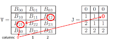
Figure 1: A schematic of evaluation of J[1][2] for the examplary matrix described in the text. First it is checked V[1][2] hold $B_{12}$. Then the indices of $B_{12}$ are transposed to get $B_{21}$ and since the latter is stored in V in column 0, J[1][2] $=0$.

and its full form reads

$$\mathtt{J}=\begin{array}[]{|c|c|c|}\hline\cr 0&0&0\\ \hline\cr 1&1&0\\ \hline\cr 2&1&1\\ \hline\cr 2&2&2\\ \hline\cr\end{array}\;.$$

To access $\hat{B}$ by rows one can simply use the ELL format, i.e., arrays V and I. To access a column $k$ of $\hat{B}$, one first reads the entries in row $k$ of array I, which in this case identify the row numbers of nonzero entries in this column. These row numbers are then used as row indices into V, with column indices read from J.

If $\hat{B}$ is not structurally symmetric, i.e. if $B_{ij}\neq 0$ and $B_{ji}=0$ for some $i,j$, then the value of $A_{ji}$ is stored in $C$ $(C_{ji}=A_{ji})$ and $A_{ij}$ is stored at $V_{ik}$ with some $0\leq k<K$. This can be indicated in the computer representation by assigning a negative value to $J_{ik}$. In a similar way the computer representation of $C$ stores the information that $A_{ij}$ is to be found in $\hat{B}$.

Note that while arrays I and J facilitate column accesses to a matrix, these accesses rely on indirect addressing, which results in uncoalesced, inefficient memory transfers. The only way to improve this would be to store a transposed matrix besides the original one, but this would require not only extra storage, but also a costly matrix transposition to be repeated every time a new matrix is assembled. In contrast, arrays I and J can be initialized only once in the program and be shared by all data related to the faces. Note also that arrays I and J could be combined into a single integer array, Q, to reduce memory requirements of the program. For example, $I_{ij}$ and $J_{ij}$ can be encoded in $Q_{ij}$ as $N\times$I${}_{ij}+$ J_ij or $K\times$J${}_{ij}+$ I_ij, with trivial decoding of $I_{ij}$ and $J_{ij}$ through integer division and remainder operations.

While in the original hybrid format $\hat{C}$ is represented in the COO format, we used compressed row sparse (CRS) instead to further reduce the memory usage. However, this particular choice does not seem to influence the overall performance significantly. Most of the polyhedrons forming the mesh are of the same simple shape, e.g., they are tetrahedra or parallelepipeds. This means that most cells have the same number of neighbours, typically 4 or 6. This, in turn, implies that most of the entries in $\hat{A}$ can fit into $\hat{B}$, with $\hat{C}$ containing only a small fraction of nonzero entries in $\hat{A}$. In particular, $\hat{C}$ usually vanishes altogether for structured meshes.

4 Results

4.1 Test cases

To validate the code and evaluate its performance we solved three CFD problems: a steady flow in a 3D lid-driven cavity [23], the transient Poiseuille flow [28] in two dimensions, and the steady flow through the human left coronary artery (LCA) (see Fig. 2 a–c). The cavity was a cube of side length $\textrm{L}=0.1$ m. A constant velocity $u_{\mathrm{lid}}=1$ m/s was imposed at its top face and the kinematic viscosity $\nu=0.01$ m²/s was assumed (Reynolds number ${\mathrm{Re}=10}$). To evaluate how the solver performance depends on the problem size, we varied the regular mesh resolution from $10^{3}$ to $223^{3}$ cells (see Tab. 1).

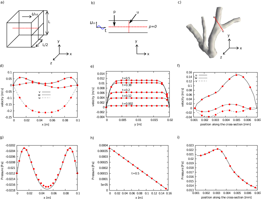
Figure 2: (Color online) Validation cases: a) lid-driven cavity ($10^{6}$ cells), b) transient Poiseuille flow, c) coronary artery. The dotted (online: red) line is the cross-section along which the results are evaluated. Results: d,f) velocity components $u$, $v$, $w$ (parallel to the $x$, $y$ and $z$ axis, respectively) along the cross-section; e) velocity $u$ at several times (in seconds); g,h,i) pressure along the cross-section. The results obtained on the CPU and GPU are shown as symbols ($\bullet$) and solid lines, respectively. Only part of the available CPU data are shown for clarity.

Table 1: Basic parameters of the meshes

Case name	Cells	Faces	Structured?
cav$10^{3}$	$1~{}000$	$3~{}300$	yes
cav$47^{3}$	$103~{}823$	$318~{}096$	yes
cav$100^{3}$	$1~{}000~{}000$	$3~{}030~{}000$	yes
cav$181^{3}$	$5~{}929~{}741$	$17~{}887~{}506$	yes
cav$223^{3}$	$11~{}089~{}567$	$33~{}417~{}888$	yes
tp$1$M	$960~{}000$	$3~{}843~{}500$	yes
lca$0.5$M	$458~{}861$	$1~{}071~{}019$	no

In the transient Poiseuelle flow (tp1M in Tab. 1) we defined a 2D pipe of length $0.16$ m and height $0.02$ m and assumed $\nu=3.3\times 10^{-6}$ m²/s. The mesh resolution was $3200\times 300$ cells. We assumed a time-dependent inlet velocity:

$$u_{\mathrm{in}}(t)=u_{0}\sin(2\pi ft)$$

with $u_{0}=0.01$ m/s and $f=0.5$ s^-1, and the zero-pressure boundary condition at the outlet. In this case we ran $5000$ PISO steps with $\delta t=0.1$ ms.

Geometry of the artery simulated in the lca0.5M case (Tab. 1) is visualised in Fig. 2c. We used $\nu=3\cdot 10^{-6}$ m²/s and assumed a constant mass flow at the inlet ($Q=9.975\times 10^{-4}$ kg/s). We imposed the zero-pressure boundary conditions in all the outlets and no-slip boundary conditions at artery walls. A non-uniform and non-orthogonal mesh built of $458~{}861$ cells was used. To solve this case, we ran $350$ iterations of SIMPLE and $2000$ iterations of PISO solvers, the latter with $\delta t=0.1$ ms.

4.2 Validation

To validate our GPU implementations we compared its solutions for all scenarios described in Sec. 4.1 to the results obtained with the OpenFOAM toolkit [27] running on the CPU. OpenFOAM was run with the same internal algorithms and control parameters as the GPU code except for the sparse unsymmetric linear solver: in the GPU code we used BiCGSTAB, whereas OpenFOAM uses BiCG. All computations were done in double precision.

Results are depicted in Fig. 2. Panels (a), (b), and (c) show the geometry of the test cases: cavity, Poiseuille and LCA, respectively. Panels (d) and (f) show the Cartesian components of the velocity, panel (e) presents the velocity component parallel to pipe walls at several times, and panels (g), (h), and (i) show the pressures. Data for the cavity and LCA were computed using the SIMPLE solver, whereas for Poiseuille problem PISO was used.

In general, one can see very good matching of the GPU and CPU results. Only a slight disagreement in the minimum value of the pressure in a cavity flow was found (see Fig. 2g). This discrepancy is marginal (results differ on the fourth significant digit), and we attribute it to the fact that different solvers for nonsymmetric sparse systems were used.

4.3 Performance evaluation

Performance tests of the GPU code were done on the Tesla C2070 graphics accelerator attached to a PC running 64-bit Ubuntu 10.04 LTS, graphics driver v. 290.10, Nvidia CUDA 4.1 and gcc 4.4.3. The reference CPU tests were performed using OpenFOAM v. 1.7 on the Intel Xeon X5670 processor, which is a 6-core chip with hyperthreading. For this reason we compared a single GPU accelerator with a single CPU processor running 12 threads. Moreover, since our GPU code relies on a very simple Jacobi (diagonal) preconditioning, we also repeated all CPU tests using the geometric-algebraic multi-grid solver (GAMG), which is considered to be among the fastest solvers of the pressure equation available in OpenFOAM.

4.3.1 Time to solution

We define the solver performance as the total time to solution, including the time necessary to read the test case definition from a disk. To find it, we ran GPU and CPU (OpenFOAM) solvers until residuals in the pressure and velocity solvers dropped below a given threshold, typically $10^{-5}$ for smaller and $10^{-4}$ for larger cases. Depending on the problem size, this time varied from 1 second to almost 31 hours. Similarly, we define the effective GPU acceleration as the ratio of the GPU solver performance to its CPU counterpart.

Figure 3a shows the effective acceleration when the GPU and CPU solvers use essentially the same algorithms and control parameters, the only exception being the BiCG solver rather than BiCGStab used by OpenFOAM to solve the velocity equations.

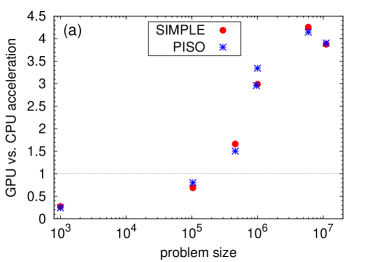
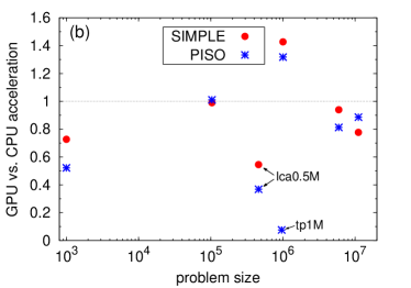
Figure 3: Acceleration of the GPU relative to the CPU (OpenFOAM) implementations of SIMPLE and PISO solvers. In all cases the linear solvers used by the GPU were Jacobi-preconditioned BiCGStab and CG. The CPU implementation used BiCG and CG with Jacobi preconditioner (a) or GAMG with the FDIC preconditioner (b).

As expected, in this case the relative performance of the GPU and CPU implementations depends strongly on the problem size. The GPU is slower than the CPU if a mesh has less than approximately $N=10^{5}$ cells, and is significantly faster, up to about 4.2 times, if $N$ is of order of a million or more. This reflects the fact that the GPU is a massively parallel device that needs tens of thousands of threads for efficient program execution. One can also see that the relative GPU-CPU performance is similar for the PISO and SIMPLE solvers.

Comparison of the GPU implementations with OpenFOAM exploiting the GAMG pressure solver is depicted in Fig. 3b. In this case the GPU can deliver a small performance gain (about 30%–40%) only for the cav$100^{3}$ case. The major factor affecting the relative GPU-CPU performance is now the structure of the problem rather than just its size: GAMG turns out much more efficient for lca0.5M and tp1M cases than for the driven cavity. This is directly related to the fact that for the former problems a Jacobi-preconditioned CG solver used in the GPU implementation needs a large number of iterations to converge, see Tab. 2. In the extreme case of the transient Poiseuille flow, tp1M, the CG solver requires almost $700$ times more iterations than GAMG. Even though GAMG iterations are far more complex, a GAMG-based PISO solver running on the CPU turns out $13$ times faster than its CG-based counterpart running on the GPU.

Table 2: Cumulative number of the pressure solver iterations: Jacobi-preconditioned CG (GPU and CPU) and GAMG (CPU).

Case	GPU-CG	CPU-CG	CPU-GAMG
SIMPLE
cav$10^{3}$	$2~{}468$	$2~{}474$	$269$
cav$47^{3}$	$122~{}216$	$103~{}321$	$3~{}699$
cav$100^{3}$	$635~{}086$	$629~{}182$	$14~{}721$
cav$181^{3}$	$1~{}424~{}531$	$1~{}618~{}634$	$29~{}191$
cav$223^{3}$	$1~{}733~{}366$	$1~{}766~{}484$	$27~{}220$
lca$0.5$M	$157~{}176$	$159~{}959$	$1~{}704$
PISO
cav$10^{3}$	$104~{}972$	$110~{}614$	$10~{}507$
cav$47^{3}$	$575~{}153$	$568~{}388$	$16~{}549$
cav$100^{3}$	$1~{}255~{}664$	$1~{}352~{}614$	$25~{}257$
cav$181^{3}$	$2~{}726~{}289$	$3~{}010~{}947$	$43~{}760$
cav$223^{3}$	$3~{}705~{}806$	$3~{}716~{}480$	$100~{}279$
lca$0.5$M	$1~{}770~{}672$	$1~{}830~{}437$	$9~{}875$
tp1M	$24~{}117~{}157$	$27~{}042~{}577$	$34~{}589$

The values in the second and third column of Tab. 2 differ by up to about 10% even though they refer to essentially the same quantity. This reflects the fact that the GPU and CPU implementations are not equivalent, as they use different linear solvers for velocity equations. Moreover, the order in which floating point operations are executed in both architectures is different, which leads to architecture-specific accumulation of numerical errors and divergent program execution.

4.3.2 Profiling

Profiling large-scale GPU code can be quite problematic. On the one hand, CPU-oriented profilers, like oprofile, usually find it difficult to distinguish calls to different CUDA functions. On the other hand, CUDA-specific profilers, like Nvidia Visual Profiler, are designed to provide fine-grained information on kernel execution (such as branch divergence or non-coalesced device memory accesses), and can incur prohibitive runtime overhead. Therefore we used a different strategy—since each GPU kernel must be launched from the CPU host, we modified the CPU source code by inserting calls to gettimeofday system timer.

Figure 4 shows the fraction of the total computation time the GPU-accelerated PISO and SIMPLE solvers spent in CG and BiCGStab linear solvers. As expected, the Jacobi-preconditioned CG solver turned out the most time-consuming part of our CFD solvers, a single factor limiting the overall performance in all but the smallest cases. Other major components of our implementation, including the Jacobi-preconditioned BiCGStab solver of sparse nonsymmetric linear systems, are negligible from the performance point of view. This is no surprise, as our implementation of the CG solver uses the simplest nontrivial preconditioner, characterized by a poor convergence rate. This, in turn, can lead to huge numbers of internal CG iterations listed in Tab. 2.

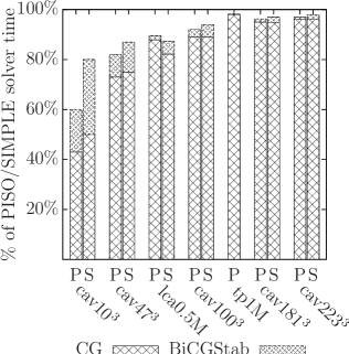
Figure 4: Percentage of the time spent in CG and BiCGStab linear solvers during a full PISO (P) and SIMPLE (S) solver execution.

As the data in Fig. 3 show that in some cases our GPU implementation is competitive to an algorithmically different, highly optimized CPU implementation, one might ask whether it is possible to improve the relative GPU-CPU performance simply by improving the GPU implementation of the Jacobi-preconditioned CG solver. To answer this question, we profiled the CG solver and show the results in Fig. 5.

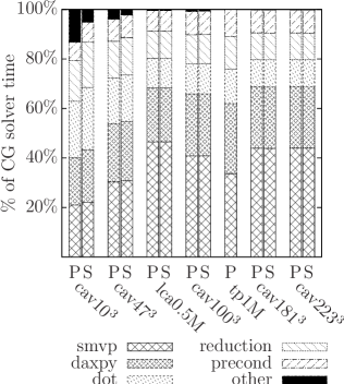
Figure 5: Percentage of the time spent in the main components of the Jacobi-preconditioned CG solver PISO (P) and SIMPLE (S).

Six groups of elementary numerical operations were investigated: SMVP (sparse matrix dense vector multiplication), daxpy (scalar times vector plus vector, $\vec{y}=\alpha\cdot\vec{x}+\vec{y}$), dot product, reduction, diagonal preconditioner, and all other operations (e.g. memory allocation and management). Since all five explicitly listed operations take at least 10% of the total CG solver time, significant improvement of the solver performance would require significant improvements in practically all of the solver components. However, as many of them (SMVP, daxpy, dot product) are memory-bound and are already highly optimized, no further significant improvement seems possible without additional hardware support.

4.3.3 Matrix assembly

While the time to solution for the cases considered in this study turned out completely dominated by the CG solver, this need not be so in other cases, other implementations, or other CFD solvers. Therefore we also profiled elementary steps of the linear matrix assembly stage. We considered three such operations: Laplacian, divergence, and gradient and compared their execution times with that of the SMVP, as all these operations are algorithmically similar. The results are collected in Tab. 3.

Table 3: Computation time of elementary matrix assembly operations in SIMPLE and PISO solvers. The data for the divergence, gradient and Laplacian are normalized relative to the SMVP time. The last column shows orthogonality of the mesh.

Case	SMVP time	Normalized time			Orth.
	[µs]	div.	grad.	Lap.
cav$10^{3}$	$41$	$3.6$	$16.8$	$2.3$	yes
cav$47^{3}$	$139$	$4.1$	$18.3$	$2.5$	yes
cav$100^{3}$	$1~{}103$	$2.9$	$10.7$	$2.4$	yes
cav$181^{3}$	$6~{}763$	$2.5$	$9.1$	$2.3$	yes
cav$223^{3}$	$12~{}620$	$2.5$	$9.0$	$2.3$	yes
lca$0.5$M	$708$	$2.6$	$12.1$	$58.7$	no
tp1M	$775$	$2.8$	$10.4$	$2.3$	yes

On can see that for orthogonal meshes the matrix assembly time is dominated by the gradient. This is a GPU-specific phenomenon, a consequence of the fact that in this operator the faces are accessed in a different order than in SMVP, which leads to uncoalesced memory accesses and significant overall performance degradation. For nonorthogonal meshes the Laplacian requires additional, costly corrections and dominates the matrix assembly time.

4.3.4 Memory usage

The largest problem we were able to run on a 6 GB device, cav223³, occupied 5.9 GB for the PISO and 5.7 GB for the SIMPLE solver, respectively. In each test case the device memory footprint was similar for PISO and SIMPLE and, for problems of size $\gtrsim 10^{5}$, equaled to $\approx 540$ bytes per cell.

5 Discussion

Our results show that a GPU can outperform a six-core server-class CPU running algorithmically equivalent implementations of popular CFD solvers, SIMPLE or PISO, by a factor slightly exceeding 4. This value is consistent with the ratio 4.5 of the theoretical memory bandwidths of the two processors used in our test, 144 GB/s (GPU) and 32 GB/s (CPU).

We show, however, that despite its huge computational power, the GPU is still inferior to the CPU if the latter uses the most efficient algorithms. This is because the GPU is not flexible enough to allow both direct and efficient implementation of many procedures optimized for CPUs. For example, some of the most efficient preconditioners for the CG sparse linear solver are based on incomplete LU decomposition, which, unfortunately, has a large serial component. This issue has attracted a lot of interest. Recently, Naumov showed a $2\times$ speedup over a quad-core CPU in the incomplete-LU preconditioned iterative methods [18], Helfenstein and Koko [13] reported a 10-fold acceleration over a single-threaded CPU code, and Nvidia included ILU0-class preconditioners in its forthcoming cusparse 5.0 GPU library [19]. Even better results for the pressure solver performance can often be achieved with multigrid methods and the effort to produce efficient GPU implementation of such solvers is also intensive, see for example Geveler et al. [11] and references therein. In particular, Geveler et al. reported a 5$\times$ average speedup over a multithreaded CPU code. These achievements are mostly concentrated on accelerating a particular, rather narrow aspect of a CFD solver. By replacing in our code the Jacobi-peconditioned CG with one of the above-mentioned solutions, it should be possible to produce a fully functional CFD solver that would at least match the speed of standard CFD software running on CPUs, which is our plan for the future.

If a faster pressure solver is used in future CFD software on GPUs, the role of the remaining solver components will increase dramatically. Moreover, since the gap between the computational power of processors and the speed of the bus connecting GPU with CPU is expected to be still widening, porting of complete software rather than accelerating only its parts will become more and more desirable.

6 Conclusions

We implemented PISO and SIMPLE solvers on GPUs and investigated their main properties. The implementations are fully functional, execute completely on the GPU using double precision and support time-dependent boundary conditions and arbitrary meshes. To facilitate a complete GPU port, we proposed a generic data format for internal data storage which helps implement elementary CFD solver operations like SMVP, gradient or Laplacian. If GPU and CPU execute essentially the same algorithms, a GPU (Tesla C2070) can outperform a server-class, 6-core CPU (Intel Xeon X5670) by up to about 4.2 times. We also investigated how the acceleration scales with the problem size and estimate that the minimum problem size for which GPU can outperform CPU is $\approx 500~{}000$. Since our GPU implementation exploits a simple pressure solver, we compared our results against the CPU running SIMPLE or PISO with a state-of-the art multigrid (GAMG) pressure solver and found that a better pressure solver is needed for serious CFD applications on GPUs. We also carried out a detailed, coarse- and fine-grained profiling of our solvers, finding that their implementation is close to optimal, which confirmed again that the only way for GPUs to match the efficiency of CPUs in PISO and SIMPLE kernels is a better pressure solver.

References

- [1] R. Barrett, M. Berry, T. F. Chan, J. Demmel, J. Donato, J. Dongarra, V. Eijkhout, R. Pozo, C. Romine, and H. Van der Vorst. Templates for the Solution of Linear Systems: Building Blocks for Iterative Methods, 2nd Edition. SIAM, Philadelphia, PA, 1994.
- [2] Nathan Bell and Michael Garland. Implementing sparse matrix-vector multiplication on throughput-oriented processors. In SC ’09: Proceedings of the Conference on High Performance Computing Networking, Storage and Analysis, pages 1–11, New York, NY, USA, 2009. ACM.
- [3] J. M. Cohen and M. J. Molemaker. Parallel Computational Fluid Dynamics. Recent Advances and Future Directions, chapter A Fast Double Precision CFD Code using CUDA, pages 414–429. DEStech Publications, 2010.
- [4] Andrew Corrigan, Fernando Camelli, Rainald Löhner, and Fernando Mut. Semi-automatic porting of a large-scale fortran CFD code to GPUs. International Journal for Numerical Methods in Fluids, 69(2):314–331, 2012.
- [5] Andrew Corrigan, Fernando F. Camelli, Rainald Löhner, and John Wallin. Running unstructured grid-based CFD solvers on modern graphics hardware. International Journal for Numerical Methods in Fluids, 66(2):221–229, 2011.
- [6] Andrew Corrigan and Rainald Löhner. Semi-automatic porting of a large-scale CFD code to multi-graphics processing unit clusters. International Journal for Numerical Methods in Fluids, pages 1–11, 2011.
- [7] Erich Elsen, Patrick LeGresley, and Eric Darve. Large calculation of the flow over a hypersonic vehicle using a GPU. Journal of Computational Physics, 227(24):10148 – 10161, 2008.
- [8] Rob Farber. CUDA Application Design and Development. Morgan Kaufmann, 1 edition, 2011.
- [9] H. Ferziger and M. Peric. Computational Methods for Fluid Dynamics. Springer, 3rd edition, 2002.
- [10] Michael Garland and David B. Kirk. Understanding throughput-oriented architectures. Comm. ACM, 53(11):58–66, 2010.
- [11] M. Geveler, D. Ribbrock, D. Göddeke, P. Zajac, and S. Turek. Towards a complete FEM-based simulation toolkit on GPUs: Unstructured grid finite element geometric multigrid solvers with strong smoothers based on sparse approximate inverses. Computers & Fluids, pages –, 2012. in press.
- [12] Mark Harris. GPU Gems: Programming Techniques, Tips and Tricks for Real-Time Graphics, chapter Fast fluid dynamics simulation on the GPU, pages 637–665. Addison-Wesley, 2007.
- [13] Rudi Helfenstein and Jonas Koko. Parallel preconditioned conjugate gradient algorithm on GPU. Journal of Computational and Applied Mathematics, 236(15):3584 – 3590, 2012.
- [14] Hrvoje Jasak. Error Analysis and Estimation for the Finite Volume Method with Applications to Fluid Flows. PhD thesis, Imperial College, London, 1996.
- [15] A. Klöckner, T. Warburton, J. Bridge, and J.S. Hesthaven. Nodal discontinuous galerkin methods on graphics processors. Journal of Computational Physics, 228(21):7863 – 7882, 2009.
- [16] V. W. Lee, Ch. Kim, J. Chhugani, M. Deisher, D. Kim, A. D. Nguyen, N. Satish, M. Smelyanskiy, S. Chennupaty, P. Hammarlund, R. Singhal, and P. Dubey. Debunking the 100x GPU vs. CPU myth: an evaluation of throughput computing on CPU and GPU. SIGARCH Comput. Archit. News, 38(3):451–460, June 2010.
- [17] Z. Malecha, Ł. Mirosław, T. Tomczak, Z. Koza, M. Matyka, W. Tarnawski, and D. Szczerba. GPU-based simulation of 3D blood flow in abdominal aorta using OpenFOAM. Archives of Mechanics, 63(2):137–161, 2011.
- [18] Maxim Naumov. Incomplete-LU and Cholesky preconditioned iterative methods using CUSPARSE and CUBLAS. Technical report, Nvidia, June 2011.
- [19] Nvidia. CUDA Toolkit 5.0 CUSPARSE Library, April 2012.
- [20] E.H. Phillips, Y. Zhang, R.L. Davis, and J.D. Owens. Rapid aerodynamic performance prediction on a cluster of graphics processing units. In 47th AIAA Aerospace Sciences Meeting, pages paper no: AIAA 2009–565, 2009.
- [21] Everett H. Phillips, Roger L. Davis, and John D. Owens. Unsteady turbulent simulations on a cluster of graphics processors. In Proceedings of the 40th AIAA Fluid Dynamics Conference, number AIAA 2010-5036, June 2010.
- [22] R. Rosner. The opportunities and challenges of exascale computing. Technical report, Office of Science, U.S. Department of Energy, 2010.
- [23] P. N. Shankar and M. D. Deshpande. Fluid mechanics in the driven cavity. Annual Review of Fluid Mechanics, 32(1):93–136, 2000.
- [24] OLCF Titan, 2012. http://www.olcf.ornl.gov/titan/.
- [25] J. Tölke and M. Krafczyk. TeraFLOP computing on a desktop PC with GPUs for 3D CFD. International Journal of Computational Fluid Dynamics, 22(7):443–456, 2008.
- [26] TOP500 supercomputer sites, June 2011. http://www.top500.org/.
- [27] H. G. Weller, G. Tabor, H. Jasak, and C. Fureby. A tensorial approach to computational continuum mechanics using object-oriented techniques. Computers in Physics, 12(6):620–631, November 1998.
- [28] J. R. Womersley. Method for the calculation of velocity, rate of flow and viscous drag in arteries when the pressure gradient is known. The Journal of physiology, 127(3):553–563, 1955.