On the Feasibility of Linear Interference Alignment for MIMO Interference Broadcast Channels with Constant Coefficients

Abstract

In this paper, we analyze the feasibility of linear interference alignment (IA) for multi-input-multi-output (MIMO) interference broadcast channel (MIMO-IBC) with constant coefficients. We pose and prove the necessary conditions of linear IA feasibility for general MIMO-IBC. Except for the proper condition, we find another necessary condition to ensure a kind of irreducible interference to be eliminated. We then prove the necessary and sufficient conditions for a special class of MIMO-IBC, where the numbers of antennas are divisible by the number of data streams per user. Since finding an invertible Jacobian matrix is crucial for the sufficiency proof, we first analyze the impact of sparse structure and repeated structure of the Jacobian matrix. Considering that for the MIMO-IBC the sub-matrices of the Jacobian matrix corresponding to the transmit and receive matrices have different repeated structure, we find an invertible Jacobian matrix by constructing the two sub-matrices separately. We show that for the MIMO-IBC where each user has one desired data stream, a proper system is feasible. For symmetric MIMO-IBC, we provide proper but infeasible region of antenna configurations by analyzing the difference between the necessary conditions and the sufficient conditions of linear IA feasibility.

I Introduction

Inter-cell interference (ICI) is a bottleneck for future cellular networks to achieve high spectral efficiency, especially for multi-input-multi-output (MIMO) systems. When multiple base stations (BSs) share both the data and the channel state information (CSI), network MIMO can improve the throughput remarkably [1]. When only CSI is shared, the ICI can be avoided by the coordination among the BSs. In information theoretic terminology, the scenario without the data sharing is a MIMO interference broadcast channel (MIMO-IBC) when each BS transmits to multiple users in its serving cell with same time-frequency resource, and is a MIMO interference channel (MIMO-IC) when each BS transmits to one user in its own cell.

To reveal the potential of the interference networks, significant research efforts have been devoted to find the capacity region. To solve such a challenging problem while capturing the essential nature of the interference channel, various approaches have been proposed to characterize the capacity approximately. Degrees of freedom (DoF) is the first-order approximation of sum rate capacity at high signal-to-noise ratio regime and also called as multiplexing gain, which has received considerable attentions. When using the break-through concept of interference alignment (IA) [2], a $G$-cell MIMO-IC where each BS and each user have $M$ antennas can achieve a DoF of $M/2$ per cell [3]. For a two-cell MIMO-IBC where each cell has $K$ active users, each BS and each user have $M=K+1$ antennas, a per cell DoF of $M$ can be achieved when $K$ approaches to infinity [4]. This result is surprising, because the DoF is the same as the maximal DoF achievable by network MIMO but without data sharing among the BSs. Encouraged by such a promising performance of linear IA, many recent works strived to analyze the DoF for MIMO-IC [5, 6] and MIMO-IBC [7, 8, 9] with various settings.

For the MIMO-IC or MIMO-IBC with constant coefficients (i.e., without symbol extension over time or frequency domain), to derive the maximum DoF achieved by linear IA, it is crucial to analyze the minimum numbers of transmit and receive antennas that guarantees the IA to be feasible. Yet the feasibility analysis of linear IA for general MIMO-IC and MIMO-IBC is still an open problem since the problem was recognized in [10].

The feasibility analysis of linear IA feasibility includes finding and proving the necessary and sufficient conditions. For the necessary conditions, a proper condition was first proposed in [11] by relating the IA feasibility to the problem of determining the solvability of a system represented by multivariate polynomial equations. When the channels are generic (i.e., drawn from a continuous probability distribution), the authors in [12, 13] proved that the proper condition is one of the necessary conditions for the IA feasibility of MIMO-IC. The proper condition was then respectively provided for symmetric MIMO-IBC in [14], general MIMO-IBC in [15] and partially-connected symmetric MIMO-IBC in [16]. Besides the proper condition, another class of necessary conditions was found for MIMO-IC in [6, 17, 18] and for MIMO-IBC in [16].

To prove the sufficient conditions, two different approaches have been employed. One is to find a closed-form solution for linear IA [4, 17, 18, 19], and the other is to prove the existence of a linear IA solution [12, 13, 20, 21]. Unfortunately, the closed-form IA solutions are only available for finite cases, e.g., symmetric three-cell MIMO-IC [17, 18] and symmetric two-cell MIMO-IBC with special antenna configurations [4, 19]. To find the sufficient conditions for general cases, various methodologies were employed in [12, 13, 20, 21] to show when the IA solutions exist. These studies all indicate that, the IA solution exists when the mapping $f:\mathcal{V}\rightarrow\mathcal{H}$ is surjective [21], where $\mathcal{H}$ is the channel space and $\mathcal{V}$ is the solution space. These studies also proved that if $f$ is surjective for one channel realization $\boldsymbol{H}_{0}$, it will be surjective for generic channels with probability one. Furthermore, the authors in [12] proved that if the Jacobian matrix of $\boldsymbol{H}_{0}$ is invertible, $f$ is surjective for $\boldsymbol{H}_{0}$. Along another line, the authors in [13, 20] proved that if the first-order terms of the IA polynomial equations with $\boldsymbol{H}_{0}$ are linear independent, $f$ will be surjective for $\boldsymbol{H}_{0}$. Interestingly, the matrix composed of the first-order terms in [13, 20] happens to be the Jacobian matrix in [12]. Moreover, the matrix to check the IA feasibility in [21] is also a Jacobian matrix, though in a form different from [12]. Consequently, all the analysis in [12, 13, 20, 21] indicate that to prove the existence of the IA solution for MIMO-IC, an invertible Jacobian matrix needs to be found, either explicitly or implicitly. This conclusion is also true for MIMO-IBC.

The way to construct an invertible Jacobian matrix depends on the channel feature. So far, an invertible Jacobian matrix has only been found for single beam MIMO-IC with general configurations and multi-beam MIMO-IC in two special cases: 1) the numbers of transmit and receive antennas are divisible by the number of data streams per user [12], and 2) the numbers of transmit and receive antennas are identical [13]. For the general multi-beam MIMO-IC, and for both single and multi-beam MIMO-IBC, the problem remains unsolved, owing to their different channel features with the single beam MIMO-IC.

The Jacobian matrix of MIMO IC and MIMO-IBC has two important properties in structure: 1) sparse structure (i.e., many elements are zero) and 2) repeated structure (i.e., some nonzero elements are identical). In general, it is hard to construct an invertible matrix with the sparse structure [22]. For MIMO-IC, the study in [20] indicates that if the Jacobian matrix can be constructed as a permutation matrix (which is invertible), the linear IA is feasible. However, only for some cases, e.g., single beam MIMO-IC and the special class of multi-beam MIMO-IC considered in [12], there exists a Jacobian matrix that can be set as a permutation matrix. For other cases, due to the repeated structure, the Jacobian matrices cannot be set as permutation matrices. Until now only the authors in [13] constructed an invertible Jacobian matrix for the MIMO-IC with $M=N$, but the construction method cannot be extended to the cases beyond such a special case. In fact, when the Jacobian matrix is not able to be set as a permutation matrix, how to construct an invertible Jacobian matrix is still unknown. This hinders the analysis for finding the minimal antenna configuration to support the IA feasibility.

In this paper, we investigate the feasibility of linear IA for the MIMO-IBC with constant coefficients. The main contributions are summarized as follows.

• The necessary conditions of the IA feasibility for a general MIMO-IBC are provided and proved. Except for the proper condition, we find another kind of necessary condition, which ensures a sort of irreducible ICI to be eliminated. The existence conditions of the irreducible ICIs are provided.

• The sufficient conditions of the IA feasibility for a special class of MIMO-IBC are proved, where the numbers of transmit and receive antennas are all divisible by the number of data streams of each user. Although the considered setup is similar to the MIMO-IC in [12], the channel features of the two setups differ. For MIMO-IBC, the invertible Jacobian matrix cannot be set as a permutation matrix due to the confliction with the repeated structure. Based on the observation that the sub-matrices of the Jacobian matrix of MIMO-IBC corresponding to the transmit and receive matrices have different repeated structures, we propose a general rule to construct an invertible Jacobian matrix where the two sub-matrices are constructed in different ways.

• From the insight provided by analyzing the necessary conditions and the sufficient conditions, we provide the proper but infeasible region of antenna configuration for symmetric MIMO-IBC.

The rest of the paper is organized as follows. We describe the system model in Section II. The necessary conditions for general MIMO-IBC and the necessary and sufficient conditions for a special class of MIMO-IBC will be provided and proved in Section III and Section IV, respectively. We discuss the connection between the proper condition and the feasibility condition in Section V. Conclusions are given in the last section.

Notations: Conjugation, transpose, Hermitian transpose, and expectation are represented by $(\cdot)^{*}$, $(\cdot)^{T}$, $(\cdot)^{H}$, and $\mathbb{E}\{\cdot\}$, respectively. $\mathrm{Tr}\{\cdot\}$ is the trace of a matrix, and $\mathrm{diag}\{\cdot\}$ is a block diagonal matrix. $\otimes$ is the Kronecker product operator, $\mathrm{vec}\{\cdot\}$ is the operator that converts a matrix or set into a column vector, $\boldsymbol{I}_{d}$ is an identity matrix of size $d$. $|\cdot|$ is the cardinality of a set, $\varnothing$ denotes an empty set, and $\mathcal{A}\setminus\mathcal{B}=\{x\in\mathcal{A}|x\notin\mathcal{B}\}$ denotes the relative complement of $\mathcal{A}$ in $B$. $\exists$ means “there exists” and $\forall$ means “for all”.

II System model

Consider a downlink $G$-cell MIMO network. In cell $i$, BS_i supports $K_{i}$ users, $i=1,\cdots,G$. The $k$th user in cell $i$ (denoted by MS${}_{i_{k}}$) is equipped with $N_{i_{k}}$ antennas to receive $d_{i_{k}}$ desired data streams from BS_i, $k=1,\cdots,K_{i}$. BS_i is equipped with $M_{i}$ antennas to transmit overall $d_{i}=\sum_{k=1}^{K_{i}}d_{i_{k}}$ data streams. The total DoF to be supported by the network is $d^{\mathrm{tot}}=\sum_{i=1}^{G}d_{i}=\sum_{i=1}^{G}\sum_{k=1}^{K_{i}}d_{i_{k}}$. Assume that there are no data sharing among the BSs and every BS has perfect CSIs of all links. This is a scenario of general MIMO-IBC, and the configuration is denoted by $\prod_{i=1}^{G}(M_{i}\times\prod_{k=1}^{K_{i}}(N_{i_{k}},d_{i_{k}}))$.

The desired signal of MS${}_{i_{k}}$ can be estimated as

$$\hat{\boldsymbol{x}}_{i_{k}}= \boldsymbol{U}_{i_{k}}^{H}\boldsymbol{H}_{i_{k},i}\boldsymbol{V}_{i_{k}}\boldsymbol{x}_{i_{k}}+\sum_{l=1,l\neq k}^{K_{i}}\boldsymbol{U}_{i_{k}}^{H}\boldsymbol{H}_{i_{k},i}\boldsymbol{V}_{i_{l}}\boldsymbol{x}_{i_{l}}$$

$$+\sum_{j=1,j\neq i}^{G}\boldsymbol{U}_{i_{k}}^{H}\boldsymbol{H}_{i_{k},j}\boldsymbol{V}_{j}\boldsymbol{x}_{j}+\boldsymbol{U}_{i_{k}}^{H}\boldsymbol{n}_{i_{k}}$$ (1)

where $\boldsymbol{x}_{i_{k}}\in\mathbb{C}^{d_{i_{k}}\times 1}$ is the symbol vector for MS${}_{i_{k}}$ satisfying $\mathbb{E}\{\boldsymbol{x}_{i_{k}}^{H}\boldsymbol{x}_{i_{k}}\}=Pd_{i_{k}}$, $P$ is the transmit power per symbol, and $\boldsymbol{x}_{j}=[\boldsymbol{x}_{j_{1}}^{T},\cdots,\boldsymbol{x}_{j_{K_{i}}}^{T}]^{T}$ is the symbol vector for the $K_{j}$ users in cell $j$, ${\boldsymbol{V}}_{i_{k}}\in\mathbb{C}^{M_{i}\times d_{i_{k}}}$ is the transmit matrix for MS${}_{i_{k}}$ satisfying $\mathrm{Tr}\{{\boldsymbol{V}}_{i_{k}}^{H}{\boldsymbol{V}}_{i_{k}}\}=d_{i_{k}}$, and ${\boldsymbol{V}}_{j}=[{{{\boldsymbol{V}}_{j_{1}}},\cdots,{\boldsymbol{V}}_{j_{K_{i}}}}]$ is the transmit matrix of BS_j for the $K_{j}$ users in cell $j$, $\boldsymbol{U}_{i_{k}}\in\mathbb{C}^{N_{i_{k}}\times d_{i_{k}}}$ is the receive matrix for MS${}_{i_{k}}$, ${\boldsymbol{H}}_{i_{k},j}\in\mathbb{C}^{N_{i_{k}}\times M_{j}}$ is the channel matrix of the link from BS_j to MS${}_{i_{k}}$ whose elements are independent random variables with a continuous distribution, and ${\boldsymbol{n}}_{i_{k}}\in\mathbb{C}^{N_{i_{k}}\times 1}$ is an additive white Gaussian noise.

The received signal of each user contains the multiuser interference (MUI) from its desired BS and the ICI from its interfering BSs, which are the second and third terms in (II). Without symbol extension, the linear IA conditions [11] can be obtained from (II) as follows,

$$\mathrm{rank}\left(\boldsymbol{U}_{i_{k}}^{H}\boldsymbol{H}_{i_{k},i}\boldsymbol{V}_{i_{k}}\right) =d_{i_{k}},~{}\forall i,k$$ (2a)

$$\boldsymbol{U}_{i_{k}}^{H}\boldsymbol{H}_{i_{k},i}\boldsymbol{V}_{i_{l}} =\boldsymbol{0},~{}\forall k\neq l$$ (2b)

$$\boldsymbol{U}_{i_{k}}^{H}\boldsymbol{H}_{i_{k},j}\boldsymbol{V}_{j} =\boldsymbol{0},~{}\forall i\neq j$$ (2c)

The polynomial equation (2a) is a rank constraint to convey the desired signals for each user. It can be interpreted as a constraint in single user MIMO system: the inter-data stream interference (IDI)-free transmission constraint. (2b) and (2c) are the zero-forcing (ZF) constraints to eliminate the MUI and ICI, respectively.

Note that multiple data streams transmitted from one BS to a user undergo the same channel. This leads to two features of MIMO-IBC, according to the cases where the BS and the user are located in the same cell or in different cells, which are

• Feature 1: the desired signal and the MUI experienced at each user undergoing the same channel.

• Feature 2: the multiple ICIs generated from one BS to a user in other cell undergo the same channel even when each user only receives one desired data stream.

III Necessary Conditions for General Cases

In this section, we present and prove the necessary conditions of linear IA feasibility for general MIMO-IBC. Since the IA conditions in (2a)-(2c) are similar to MIMO-IC and the proof builds upon the same line of the work in [12], we emphasize the difference of MIMO-IBC from MIMO-IC, which comes from the first feature of MIMO-IBC.

Theorem 1 (Necessary Conditions)

For a general MIMO-IBC with configuration $\prod_{i=1}^{G}(M_{i}\times\prod_{k=1}^{K_{i}}(N_{i_{k}},d_{i_{k}}))$ where the channel matrices $\{\boldsymbol{H}_{i_{k},j}\}$ are generic (i.e., drawn from a continuous probability distribution), if the linear IA is feasible, the following conditions must be satisfied,

$$\min\{M_{i}-d_{i},N_{i_{k}}-d_{i_{k}}\}\geq 0,~{}\forall i,k$$ (3a)

$$\sum_{j:(i,j)\in\mathcal{I}}\left(M_{j}-d_{j}\right)d_{j}+\sum_{i:(i,j)\in\mathcal{I}}\sum_{k\in\mathcal{K}_{i}}\left(N_{i_{k}}-d_{i_{k}}\right)d_{i_{k}}$$

$$\geq \sum_{(i,j)\in\mathcal{I}}d_{j}\sum_{k\in\mathcal{K}_{i}}d_{i_{k}},~{}\forall\mathcal{I}\subseteq\mathcal{J}$$ (3b)

$$\max\Big{\{}\sum_{j\in\mathcal{I}_{\mathrm{A}}}M_{j},\sum_{i\in\mathcal{I}_{\mathrm{B}}}\sum_{k\in\mathcal{K}_{i}}N_{i_{k}}\Big{\}}$$

$$\geq \sum_{j\in\mathcal{I}_{\mathrm{A}}}d_{j}+\sum_{i\in\mathcal{I}_{\mathrm{B}}}\sum_{k\in\mathcal{K}_{i}}d_{i_{k}},~{}\forall\mathcal{I}_{\mathrm{A}}\cap\mathcal{I}_{\mathrm{B}}=\varnothing$$ (3c)

where $\mathcal{K}_{i}\subseteq\{1,\cdots,K_{i}\}$ is an arbitrary subset of the users in cell $i$, $\mathcal{J}=\{(i,j)|1\leq i\neq j\leq G\}$ denotes the set of all cell-pairs that mutually interfering each other, $\mathcal{I}$ is an arbitrary subset of $\mathcal{J}$, and $\mathcal{I}_{\mathrm{A}},~{}\mathcal{I}_{\mathrm{B}}\subseteq\{1,\cdots,G\}$ are arbitrary two subsets of the index set of the $G$ cells.

III-A Proof of (3a)

Proof:

Comparing (2a) and (2b), we can see that the channel matrices of MS${}_{i_{k}}$ in the two equations are all equal to $\boldsymbol{H}_{i_{k},i}$. As a result, the rank constraint is coupled with the MUI-free constraint, such that the proof for MIMO-IC in [10, 11] cannot be directly applied.

Note that from the view of MS${}_{i_{k}}$, the desired data streams of other users in cell $i$ are its MUI, while from the view of BS_i, all the data streams for the users in cell $i$ are its desired signals. Combining (2a) and (2b), we can obtain a rank constraint for BS_i as $\mathrm{rank}\left([\boldsymbol{H}_{i_{1},i}^{H}\boldsymbol{U}_{i_{1}},\cdots,\boldsymbol{H}_{i_{K_{i}},i}^{H}\boldsymbol{U}_{i_{K_{i}}}]^{H}\boldsymbol{V}_{i}\right)=\sum_{k=1}^{K_{i}}d_{i_{k}}=d_{i}$. Then, the IA conditions in (2a)$-$(2c) can be equivalently rewritten as

$$\mathrm{rank}\left(\left[\begin{array}[]{ccc}\boldsymbol{U}_{i_{1}}^{H}&{}\hfil&{\boldsymbol{0}}\\ {}\hfil&\ddots&{}\hfil\\ {\boldsymbol{0}}&{}\hfil&\boldsymbol{U}_{i_{K_{i}}}^{H}\end{array}\right]\left[\begin{array}[]{c}\boldsymbol{H}_{i_{1},i}\\ \vdots\\ \boldsymbol{H}_{i_{K_{i}},i}\end{array}\right]\boldsymbol{V}_{i}\right) =d_{i},~{}\forall i$$ (4g)

$$\boldsymbol{U}_{i_{k}}^{H}\boldsymbol{H}_{i_{k},j}\boldsymbol{V}_{j} =\boldsymbol{0},~{}\forall i\neq j$$ (4h)

Now the channel matrices in (4g) are independent of those in (4h). Since the channel matrix $\boldsymbol{H}_{i_{k},i}$ is generic, (4g) is automatically satisfied with probability one when $\mathrm{rank}(\boldsymbol{V}_{i})=d_{i}$ and $\mathrm{rank}(\boldsymbol{U}_{i_{k}})=d_{i_{k}}$[10]. Therefore, (3a) is necessary to satisfy the equivalent rank constraint (4g). ∎

Different from multi-beam MIMO-IC, the aggregated receive matrix for different users in MIMO-IBC has a block-diagonal structure due to the non-cooperation among the users.

The intuitive meaning of (3a) is straightforward. BS_i should have enough antennas to transmit the overall $d_{i}$ desired signals to multiple users in cell $i$, i.e., to ensure MUI-free transmission, and MS${}_{i_{k}}$ should have enough antennas to receive its $d_{i_{k}}$ desired signals, i.e., to ensure IDI-free transmission.

III-B Proof of (3)

Proof:

To satisfy (4h) under the constraint of (4g), we need to first reserve some variables in the transmit and receive matrices to ensure the equivalent rank constraints, and then use the remaining variables to remove the ICI. To this end, we partition the transmit and receive matrices as follows

$$\boldsymbol{V}_{j} =\boldsymbol{P}_{j}^{V}\left[\begin{array}[]{c}\boldsymbol{I}_{d_{j}}\\ \bar{\boldsymbol{V}}_{j}\end{array}\right]\boldsymbol{Q}_{j}^{V},\quad\boldsymbol{U}_{i_{k}}=\boldsymbol{P}_{i_{k}}^{U}\left[\begin{array}[]{c}\boldsymbol{I}_{d_{i_{k}}}\\ \bar{\boldsymbol{U}}_{i_{k}}\end{array}\right]\boldsymbol{Q}_{i_{k}}^{U}$$ (9)

where $\boldsymbol{P}_{j}^{V}\in\mathbb{C}^{M_{j}\times M_{j}}$ and $\boldsymbol{P}_{i_{k}}^{U}\in\mathbb{C}^{N_{i_{k}}\times N_{i_{k}}}$ are square permutation matrices, $\boldsymbol{Q}_{j}^{V}\in\mathbb{C}^{d_{j}\times d_{j}}$ and $\boldsymbol{Q}_{i_{k}}^{U}\in\mathbb{C}^{d_{i_{k}}\times d_{i_{k}}}$ are invertible matrices, and $\bar{\boldsymbol{V}}_{i}\in\mathbb{C}^{(M_{j}-d_{j})\times d_{j}}$ and $\bar{\boldsymbol{U}}_{i_{k}}\in\mathbb{C}^{(N_{i_{k}}-d_{i_{k}})\times d_{i_{k}}}$ are the effective transmit and receive matrices, whose elements are the remaining variables after extracting $d_{j}^{2}$ and $d_{i_{k}}^{2}$ variables of ${\boldsymbol{V}}_{j}$ and ${\boldsymbol{U}}_{i_{k}}$, respectively.

Then, (4h) can be rewritten as

$$\left(\boldsymbol{Q}_{i_{k}}^{U}\right)^{H}\left[\begin{array}[]{cc}\boldsymbol{I}_{d_{i_{k}}}&\bar{\boldsymbol{U}}_{i_{k}}^{H}\end{array}\right]\underbrace{\left(\boldsymbol{P}_{i_{k}}^{U}\right)^{H}\boldsymbol{H}_{i_{k},j}\boldsymbol{P}_{j}^{V}}_{\bar{\boldsymbol{H}}_{i_{k},j}}\left[\begin{array}[]{c}\boldsymbol{I}_{d_{j}}\\ \bar{\boldsymbol{V}}_{j}\end{array}\right]\boldsymbol{Q}_{j}^{V}=\boldsymbol{0}$$ (13)

where $\bar{\boldsymbol{H}}_{i_{k},j}=\left(\boldsymbol{P}_{i_{k}}^{U}\right)^{H}\boldsymbol{H}_{i_{k},j}\boldsymbol{P}_{j}^{V}$ is the effective channel matrix.

Further partition the effective channel matrix as follows

$$\bar{\boldsymbol{H}}_{i_{k},j}=\left[\begin{array}[]{cc}\bar{\boldsymbol{H}}_{i_{k},j}^{(1)}&\bar{\boldsymbol{H}}_{i_{k},j}^{(2)}\\ \bar{\boldsymbol{H}}_{i_{k},j}^{(3)}&\bar{\boldsymbol{H}}_{i_{k},j}^{(4)}\end{array}\right]$$

where $\bar{\boldsymbol{H}}_{i_{k},j}^{(1)}\in\mathbb{C}^{d_{i_{k}}\times d_{j}}$, $\bar{\boldsymbol{H}}_{i_{k},j}^{(2)}\in\mathbb{C}^{d_{i_{k}}\times(M_{j}-d_{j})}$, $\bar{\boldsymbol{H}}_{i_{k},j}^{(3)}\in\mathbb{C}^{(N_{i_{k}}-d_{i_{k}})\times d_{j}}$ and $\bar{\boldsymbol{H}}_{i_{k},j}^{(4)}\in\mathbb{C}^{(N_{i_{k}}-d_{i_{k}})\times(M_{j}-d_{j})}$, respectively.

Then, (13) is equivalent to the following equation,

$$\left[\begin{array}[]{cc}\boldsymbol{I}_{d_{i_{k}}}&\bar{\boldsymbol{U}}_{i_{k}}^{H}\end{array}\right]\left[\begin{array}[]{cc}\bar{\boldsymbol{H}}_{i_{k},j}^{(1)}&\bar{\boldsymbol{H}}_{i_{k},j}^{(2)}\\ \bar{\boldsymbol{H}}_{i_{k},j}^{(3)}&\bar{\boldsymbol{H}}_{i_{k},j}^{(4)}\end{array}\right]\left[\begin{array}[]{c}\boldsymbol{I}_{d_{j}}\\ \bar{\boldsymbol{V}}_{j}\end{array}\right]=\boldsymbol{0}$$ (19)

Now the IA conditions in (4g) and (4h) turns into a single condition.

From (19), the relationship between the effective transmit and receive matrices and the effective channel matrices can be expressed in the form of implicit function, i.e.,

$$\boldsymbol{F}_{i_{k},j}(\bar{\boldsymbol{H}};\bar{\boldsymbol{V}},\bar{\boldsymbol{U}})= \bar{\boldsymbol{H}}_{i_{k},j}^{(1)}+\bar{\boldsymbol{H}}_{i_{k},j}^{(2)}\bar{\boldsymbol{V}}_{j}+\bar{\boldsymbol{U}}_{i_{k}}^{H}\bar{\boldsymbol{H}}_{i_{k},j}^{(3)}+\bar{\boldsymbol{U}}_{i_{k}}^{H}\bar{\boldsymbol{H}}_{i_{k},j}^{(4)}\bar{\boldsymbol{V}}_{j}$$

$$= \boldsymbol{0},~{}\forall i\neq j$$ (20)

where $\boldsymbol{F}_{i_{k},j}(\cdot)$ represents the ICIs from $\bar{\boldsymbol{V}}_{j}$ to $\bar{\boldsymbol{U}}_{i_{k}}$, i.e., the interference generated by the effective transmit matrix of BS_j to the $k$th user in cell $i$.

In (III-B), $\boldsymbol{F}_{i_{k},j}(\cdot)\in\mathbb{C}^{d_{i_{k}}\times d_{j}}$ includes $d_{j}d_{i_{k}}$ ICIs, and $\bar{\boldsymbol{V}}_{j}$ and $\bar{\boldsymbol{U}}_{i_{k}}$ provide $(M_{j}-d_{j})d_{j}$ and $(N_{i_{k}}-d_{i_{k}})d_{i_{k}}$ variables, respectively. Hence, (3) ensures that for all subsets of the equations in (III-B), the number of involved variables is at least as large as the number of corresponding equations. Analogous to MIMO-IC, to eliminate the ICI in the network thoroughly, all the cell-pairs that are interfering each other, i.e., those in set $\mathcal{J}$ and any subset of it, $\mathcal{I}$, should be considered. Different from MIMO-IC, we should not generate ICI to arbitrary subsets of the users in each cell, i.e., $\mathcal{K}_{i}$, rather than not generate ICI to a single user in each cell.

From the definition in [11], we know that this is actually the condition to ensure the MIMO-IBC to be proper. In a MIMO-IC with generic channel matrix, the proper condition has been proved as a necessary condition of the IA feasibility [12]. For the considered MIMO-IBC, the channel matrix $\boldsymbol{H}_{i_{k},j}$ is also generic. Therefore, the proper condition is necessary for the MIMO-IBC to be feasible. Now, (3) is proved. ∎

The intuitive meaning of (3) is to ensure that any pairs of BSs and the users in any pairs of cells should have enough spatial resources to transmit and receive their desired signals and to eliminate the ICIs between these BSs and users.

III-C Proof of (3)

Proof:

To express the ICIs generated from the BSs in any cells to the users in any other cells, we consider two non-overlapping clusters A and B, as shown in Fig. 1. We use $\mathcal{I}_{\mathrm{A}}$ and $\mathcal{I}_{\mathrm{B}}$ to denote the cell index sets in the clusters A and B, respectively, then $\mathcal{I}_{\mathrm{A}}\cap\mathcal{I}_{\mathrm{B}}=\varnothing$. Let $\mathcal{A}=\{j|j\in\mathcal{I}_{\mathrm{A}}\}$ and $\mathcal{B}=\{i_{k}|k\in\mathcal{K}_{i},~{}i\in\mathcal{I}_{\mathrm{B}}\}$ denote the BS index set in cluster A and the user index set in cluster B, respectively. The ZF constraints to eliminate the ICI from the BSs in cluster A to the users in cluster B can be written as

$$\boldsymbol{U}_{\mathrm{B}}^{H}\boldsymbol{H}_{\mathrm{B},\mathrm{A}}\boldsymbol{V}_{\mathrm{A}}=\boldsymbol{0}$$ (21)

where $\boldsymbol{V}_{\mathrm{A}}=\mathrm{diag}\{\boldsymbol{V}_{A_{1}},\cdots,\boldsymbol{V}_{A_{p}}\}\in\mathbb{C}^{d_{\mathrm{A}}\times M_{\mathrm{A}}}$, $\boldsymbol{U}_{\mathrm{B}}=\mathrm{diag}\{\boldsymbol{U}_{B_{1}},\cdots$, $\boldsymbol{U}_{B_{q}}\}\in\mathbb{C}^{d_{\mathrm{B}}\times N_{\mathrm{B}}}$,

$$\boldsymbol{H}_{\mathrm{B},\mathrm{A}}=\left[\begin{array}[]{ccc}\boldsymbol{H}_{B_{1},A_{1}}&\cdots&\boldsymbol{H}_{B_{1},A_{p}}\\ \vdots&\ddots&\vdots\\ \boldsymbol{H}_{B_{q},A_{1}}&\cdots&\boldsymbol{H}_{B_{q},A_{p}}\end{array}\right]\in\mathbb{C}^{N_{\mathrm{B}}\times M_{\mathrm{A}}}$$

is the stacked channel matrix from the BSs in cluster A to the users in cluster B, $A_{s}$ and $B_{s}$ are the $s$th elements in $\mathcal{A}$ and $\mathcal{B}$, respectively, $p\triangleq|\mathcal{A}|=|\mathcal{I}_{\mathrm{A}}|$ and $q\triangleq|\mathcal{B}|=\sum_{i\in\mathcal{I}_{\mathrm{B}}}|\mathcal{K}_{i}|$, $d_{\mathrm{A}}=\sum_{j\in\mathcal{I}_{\mathrm{A}}}d_{j}$ is the number of all data streams transmitted from the BSs in cluster A, $d_{\mathrm{B}}=\sum_{i\in\mathcal{I}_{\mathrm{B}}}\sum_{k\in\mathcal{K}_{i}}d_{i_{k}}$ is the number of all data streams received at the users in cluster B, $M_{\mathrm{A}}=\sum_{j\in\mathcal{I}_{\mathrm{A}}}M_{j}$ is the number of all transmit antennas at the BSs in cluster A, and $N_{\mathrm{B}}=\sum_{i\in\mathcal{I}_{\mathrm{B}}}\sum_{k\in\mathcal{K}_{i}}N_{i_{k}}$ is the number of all receive antennas at the users in cluster B.

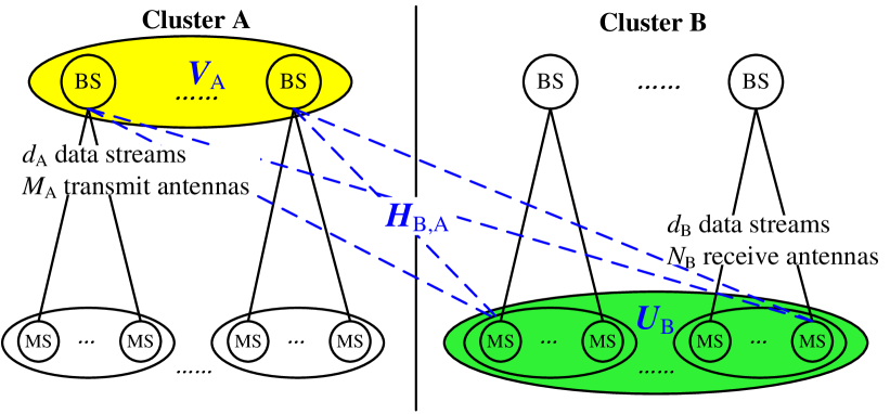
Figure 1: ICI between arbitrary two non-overlapping clusters.

Since $\boldsymbol{H}_{\mathrm{B},\mathrm{A}}$ is generic, its rank satisfies $\mathrm{rank}\left(\boldsymbol{H}_{\mathrm{B},\mathrm{A}}\right)=\min\{M_{\mathrm{A}},N_{\mathrm{B}}\}$ with probability one [10]. If $N_{\mathrm{B}}\geq M_{\mathrm{A}}$, $\mathrm{rank}\left(\boldsymbol{H}_{\mathrm{B},\mathrm{A}}\right)=M_{\mathrm{A}}\geq d_{\mathrm{A}}$. Since $\boldsymbol{H}_{\mathrm{B},\mathrm{A}}$ is independent of $\boldsymbol{V}_{\mathrm{A}}$, we have $\mathrm{rank}(\boldsymbol{H}_{\mathrm{B},\mathrm{A}}\boldsymbol{V}_{\mathrm{A}})=\mathrm{rank}(\boldsymbol{V}_{\mathrm{A}})=d_{\mathrm{A}}$ with probability one. Then, the users in cluster B will see $d_{\mathrm{A}}$ ICIs from the BSs in cluster A. On the other hand, the users in cluster B need to receive overall $d_{\mathrm{B}}$ desired signals from the BSs in cluster B, i.e., $\mathrm{rank}(\boldsymbol{U}_{\mathrm{B}})=d_{\mathrm{B}}$. To separate the ICIs from cluster A and the desired signals of cluster B, the overall subspace dimension of the received signals for the users in cluster B should satisfy $N_{\mathrm{B}}\geq d_{\mathrm{A}}+d_{\mathrm{B}}$ according to the rank-nullity theorem [23].

Similarly, if $N_{\mathrm{B}}\leq M_{\mathrm{A}}$, we have $\mathrm{rank}(\boldsymbol{U}_{\mathrm{B}}^{H}\boldsymbol{H}_{\mathrm{B},\mathrm{A}})=\mathrm{rank}(\boldsymbol{U}_{\mathrm{B}})=d_{\mathrm{B}}$ with probability one. Then, the BSs in cluster A need to avoid generating $d_{\mathrm{B}}$ ICIs to the users in cluster B. To transmit $d_{\mathrm{A}}$ desired data streams, the overall subspace dimension of the transmit signals from the BSs in cluster A should satisfy $M_{\mathrm{A}}\geq d_{\mathrm{A}}+d_{\mathrm{B}}$.

As a result, we obtain $\max\{M_{\mathrm{A}},N_{\mathrm{B}}\}\geq d_{\mathrm{A}}+d_{\mathrm{B}}$, i.e., (3). ∎

The intuitive meaning of (3) is to ensure that a sort of irreducible ICI can be eliminated. The concept of irreducible ICI is explained as follows. For the ICIs between a BS in cluster A and a set of users in cluster B, if the dimension of these ICIs cannot be reduced by designing the receive matrices of the users, they are irreducible ICIs and can only be eliminated by the BS. Similarly, for the ICIs between several BSs in cluster A and a user in cluster B, if the dimension of these ICIs cannot be reduced by designing the transmit matrices of the BSs, they are irreducible ICIs and can only be eliminated by the user.

From the proof of (3), we know that when

$$M_{j}\geq\sum_{i\in\mathcal{I}_{\mathrm{B}}}\sum_{k\in\mathcal{K}_{i}}N_{i_{k}},\quad~{}\exists\mathcal{I}_{\mathrm{B}}\subseteq\{1,\cdots,G\}\setminus\{j\}$$ (22)

$\mathrm{rank}(\boldsymbol{U}_{\mathrm{B}}^{H}\boldsymbol{H}_{\mathrm{B},\mathrm{A}})=\mathrm{rank}(\boldsymbol{U}_{\mathrm{B}})=d_{\mathrm{B}}$ always holds. It implies that when there exists a BS in cluster A whose dimension of observation space is no less than the overall dimension of observation space at all the users in cluster B, there exist the irreducible ICIs that can only be removed by the BS.

On the other hand, when

$$N_{i_{k}}\geq\sum_{j\in\mathcal{I}_{\mathrm{A}}}M_{j},~{}\exists\mathcal{I}_{\mathrm{A}}\subseteq\{1,\cdots,G\}\setminus\{i\}$$ (23)

$\mathrm{rank}(\boldsymbol{H}_{\mathrm{B},\mathrm{A}}\boldsymbol{V}_{\mathrm{A}})=d_{\mathrm{A}}$ always holds, i.e., there exist the irreducible ICIs that can only be removed by the user.

Therefore, we call (22) and (23) as the existence conditions of the irreducible ICIs.

To understand the impact of the irreducible ICIs, we take the case satisfying (22) as an example, where the ICIs between BS_j and the users in cluster B are irreducible. In other words, the receive matrices of the users in cluster B are not able to compress these ICIs. To ensure the linear IA to be feasible, in this case (3) requires $M_{j}\geq d_{j}+\sum_{i\in\mathcal{I}_{\mathrm{B}}}\sum_{k\in\mathcal{K}_{i}}d_{i_{k}}$, which is equivalent to

$$(M_{j}-d_{j})d_{j}\geq d_{j}\sum_{i\in\mathcal{I}_{\mathrm{B}}}\sum_{k\in\mathcal{K}_{i}}d_{i_{k}}$$ (24)

It means that the number of variables in the effective transmit matrix at BS_j should exceed the number of ICIs. In other words, BS_j should be able to avoid the ICI. Therefore, (24) is the condition of eliminating the irreducible ICI.

By contrast, if (22) does not hold, these ICIs are reducible at the BS passively, because anyway the BS only “see” these ICIs in a subspace with lower dimension of $M_{j}$ than the overall observation space at all the users in cluster B with dimension of $\sum_{i\in\mathcal{I}_{\mathrm{B}}}\sum_{k\in\mathcal{K}_{i}}N_{i_{k}}$. In this case, the ICIs between BS_j and the users in cluster B can be removed by their implicit “cooperation” of sharing variables in their processing matrices. To eliminate the ICI from BS_j to the users in cluster B, in this case the proper condition (3) requires

$$(M_{j}-d_{j})d_{j}+\sum_{i\in\mathcal{I}_{\mathrm{B}}}\sum_{k\in\mathcal{K}_{i}}(N_{i_{k}}-d_{i_{k}})d_{i_{k}}\geq d_{j}\sum_{i\in\mathcal{I}_{\mathrm{B}}}\sum_{k\in\mathcal{K}_{i}}d_{i_{k}}$$ (25)

It indicates that the overall number of variables in the transmit and receive matrices at both BS_j and the users in set $\mathcal{K}_{i}$ should exceed the overall number of ICIs among them. Therefore, (25) is the condition of eliminating the reducible ICI.

In practice, there exist both the reducible ICI and the irreducible ICI in a MIMO-IBC. Comparing (24) and (25), we can see that the proper conditions only ensure to eliminate all the reducible ICIs but not all the irreducible ICIs. This explains the reason why the IA is infeasible for the system whose configuration satisfies (3) but does not satisfy (3).

In summary, (3a) ensures that there are enough antennas to convey the desired signals between each BS and each user. (3) ensures to eliminate the reducible ICIs by sharing the spatial resources between the BSs and the users, whereas (3) ensures to eliminate the irreducible ICIs either at the BS side or at the user side.

IV Necessary and Sufficient Conditions for a Special Class of MIMO-IBC

In this section, we present and prove the necessary and sufficient conditions of linear IA feasibility for a special class of MIMO-IBC, where the numbers of transmit and receive antennas are all divisible by the number of data streams of each user. Owing to the second feature of MIMO-IBC, the sufficiency proof for MIMO-IBC is more difficult than the special class of MIMO-IC in [12].

We start by proving the necessity, which is simple. Then, we analyze two important properties of the Jacobian matrix for general MIMO-IBC and MIMO-IC. We proceed to present three lemmas to show the impact of the two properties. Finally, we prove the sufficiency by constructing an invertible Jacobian matrix for the considered MIMO-IBC, i.e., find the minimal antenna configuration to ensure the IA feasibility.

Theorem 2 (Necessary and Sufficient Conditions)

For a special class of MIMO-IBC with configuration $\prod_{i=1}^{G}(M_{i}\times\prod_{k=1}^{K_{i}}(N_{i_{k}},d_{i_{k}}))$ where the channel matrices $\{\boldsymbol{H}_{i_{k},j}\}$ are generic, when $d_{i_{k}}=d$, and both $M_{i}$ and $N_{i_{k}}$ are divisible by $d$, the linear IA is feasible iff (if and only if) the following conditions are satisfied,

$$\min\{M_{i}-K_{i}d,N_{i_{k}}-d\}\geq 0,~{}\forall i,k$$ (26a)

$$\sum_{j:(i,j)\in\mathcal{I}}(M_{j}-K_{j}d)K_{j}+\sum_{i:(i,j)\in\mathcal{I}}\sum_{k\in\mathcal{K}_{i}}(N_{i_{k}}-d)$$

$$\geq \sum_{(i,j)\in\mathcal{I}}K_{j}|\mathcal{K}_{i}|d,~{}\forall\mathcal{I}\subseteq\mathcal{J}$$ (26b)

IV-A Proof of the necessity

Proof:

Comparing Theorem 1 and Theorem 2, we can see that (26a) and (26) are the reduced forms of (3a) and (3) for the special class of MIMO-IBC in Theorem 2. For this class of MIMO-IBC, (3) becomes

$$\max\Big{\{}\sum_{j\in\mathcal{I}_{\mathrm{A}}}M_{j},\sum_{i\in\mathcal{I}_{\mathrm{B}}}\sum_{k\in\mathcal{K}_{i}}N_{i_{k}}\Big{\}}$$

$$\geq \sum_{j\in\mathcal{I}_{\mathrm{A}}}K_{j}d+\sum_{i\in\mathcal{I}_{\mathrm{B}}}|\mathcal{K}_{i}|d,~{}\forall\mathcal{I}_{\mathrm{A}}\cap\mathcal{I}_{\mathrm{B}}=\varnothing$$ (27)

In the sequel, we show that (IV-A) can be derived from (26a) and (26).

Since $M_{j}$ is integral multiples of $d$, the value of $M_{j}$ can be divided into two cases:

1. $\sum_{j\in\mathcal{I}_{\mathrm{A}}}M_{j}\geq(\sum_{j\in\mathcal{I}_{\mathrm{A}}}K_{j}+\sum_{i\in\mathcal{I}_{\mathrm{B}}}|\mathcal{K}_{i}|)d$,

2. $\sum_{j\in\mathcal{I}_{\mathrm{A}}}M_{j}\leq(\sum_{j\in\mathcal{I}_{\mathrm{A}}}K_{j}+\sum_{i\in\mathcal{I}_{\mathrm{B}}}|\mathcal{K}_{i}|-1)d$.

In the first case, (IV-A) always holds. In the second case, we have

$$\sum_{i\in\mathcal{I}_{\mathrm{B}}}|\mathcal{K}_{i}|d-\sum_{j\in\mathcal{I}_{\mathrm{A}}}(M_{j}-K_{j}d)\geq d$$ (28)

Considering (26a), we know that $M_{j}-K_{j}d\geq 0$. Thus the inequality $\sum_{j\in\mathcal{I}_{\mathrm{A}}}(M_{j}-K_{j}d)\geq M_{j}-K_{j}d$ always holds. Substituting this inequality into (28), we have

$$\sum_{i\in\mathcal{I}_{\mathrm{B}}}|\mathcal{K}_{i}|d-(M_{j}-K_{j}d)\geq d$$ (29)

Considering the definition of $\mathcal{I}_{\mathrm{A}}$ and $\mathcal{I}_{\mathrm{B}}$ in (IV-A), (26) can be rewritten as $\sum_{j\in\mathcal{I}_{\mathrm{A}}}(M_{j}-K_{j}d)K_{j}+\sum_{i\in\mathcal{I}_{\mathrm{B}}}\sum_{k\in\mathcal{K}_{i}}(N_{i_{k}}-d)\\ \geq\sum_{j\in\mathcal{I}_{\mathrm{A}}}K_{j}\sum_{i\in\mathcal{I}_{\mathrm{B}}}|\mathcal{K}_{i}|d$, which is equivalent to

$$\sum_{i\in\mathcal{I}_{\mathrm{B}}}\sum_{k\in\mathcal{K}_{i}}N_{i_{k}}\geq \sum_{j\in\mathcal{I}_{\mathrm{A}}}K_{j}\Big{(}\sum_{i\in\mathcal{I}_{\mathrm{B}}}|\mathcal{K}_{i}|d-(M_{j}-K_{j}d)\Big{)}$$

$$+\sum_{i\in\mathcal{I}_{\mathrm{B}}}|\mathcal{K}_{i}|d$$ (30)

Substituting (29) into (IV-A), we obtain (IV-A). ∎

For the considered class of MIMO-IBC, since (IV-A) (i.e., (3)) can be derived from (26) (i.e., (3)), the proper condition ensures that when there exist some irreducible ICIs, the BS or the user has enough spatial resources to avoid (or cancel) them.

IV-B Proof of the sufficiency

From the analysis in [12, 13], we know that the linear IA will be feasible for general MIMO-IC and MIMO-IBC under generic channels if we can find a channel realization that has an IA solution and whose Jacobian matrix is invertible.

Consider a channel matrix as follows

$$\bar{\boldsymbol{H}}_{0i_{k},j}=\left[\begin{array}[]{cc}\boldsymbol{0}&\bar{\boldsymbol{H}}_{0~{}i_{k},j}^{(2)}\\ \bar{\boldsymbol{H}}_{0~{}i_{k},j}^{(3)}&\boldsymbol{0}\end{array}\right]$$

under which an IA solution can be easily found as

$${\boldsymbol{V}}_{0j}=\left[\begin{array}[]{c}\boldsymbol{I}_{d_{j}}\\ \boldsymbol{0}_{(M_{j}-d_{j})\times d_{j}}\end{array}\right],~{}~{}{\boldsymbol{U}}_{0i_{k}}=\left[\begin{array}[]{c}\boldsymbol{I}_{d_{i_{k}}}\\ \boldsymbol{0}_{(N_{i_{k}}-d_{i_{k}})\times d_{i_{k}}}\end{array}\right]$$

Then, to prove the sufficiency, we only need to construct a Jacobian matrix that is invertible at $\bar{\boldsymbol{H}}_{0i_{k},j}$.

Substituting $\bar{\boldsymbol{H}}_{0~{}i_{k},j}$ into (III-B), we obtain

$$\boldsymbol{F}_{i_{k},j}(\bar{\boldsymbol{H}}_{0})=\bar{\boldsymbol{H}}_{0~{}i_{k},j}^{(2)}\bar{\boldsymbol{V}}_{j}+\bar{\boldsymbol{U}}_{i_{k}}^{H}\bar{\boldsymbol{H}}_{0~{}i_{k},j}^{(3)}=\boldsymbol{0},~{}\forall i\neq j$$ (31)

By taking partial derivatives to (31), we can obtain the Jacobian matrix of $\bar{\boldsymbol{H}}_{0}$. Before constructing an invertible Jacobian matrix, we first analyze its properties.

IV-B1 Jacobian matrix: properties and impacts

To see the structure of the Jacobian matrices for general MIMO-IC and MIMO-IBC, we rewrite the matrices in (31) as $\boldsymbol{F}_{i_{k},j}(\bar{\boldsymbol{H}}_{0})=[\boldsymbol{F}_{i_{k},j_{1}}(\bar{\boldsymbol{H}}_{0}),\cdots,\boldsymbol{F}_{i_{k},j_{K_{j}}}(\bar{\boldsymbol{H}}_{0})]$, $\bar{\boldsymbol{V}}_{j}=[\bar{\boldsymbol{V}}_{j_{1}},\cdots,\bar{\boldsymbol{V}}_{j_{K_{j}}}]$, and $\bar{\boldsymbol{H}}_{0~{}i_{k},j}^{(3)}=[\bar{\boldsymbol{H}}_{0~{}i_{k},j_{1}}^{(3)},\cdots,\bar{\boldsymbol{H}}_{0~{}i_{k},j_{K_{j}}}^{(3)}]$, where $\boldsymbol{F}_{i_{k},j_{l}}(\bar{\boldsymbol{H}}_{0})\in\mathbb{C}^{d_{i_{k}}\times d_{j_{l}}}$, $\bar{\boldsymbol{V}}_{j_{l}}\in\mathbb{C}^{(M_{j}-d_{j})\times d_{j_{l}}}$, and $\bar{\boldsymbol{H}}_{0~{}i_{k},j_{l}}^{(3)}\in\mathbb{C}^{(N_{i_{k}}-d_{i_{k}})\times d_{j_{l}}}$. Then (31) can be rewritten as $K_{j}$ groups of subequations, where the $l$th subequation is

$$\boldsymbol{F}_{i_{k},j_{l}}(\bar{\boldsymbol{H}}_{0})=\bar{\boldsymbol{H}}_{0~{}i_{k},j}^{(2)}\bar{\boldsymbol{V}}_{j_{l}}+\bar{\boldsymbol{U}}_{i_{k}}^{H}\bar{\boldsymbol{H}}_{0~{}i_{k},j_{l}}^{(3)}=\boldsymbol{0},~{}\forall i\neq j$$ (32)

The Jacobian matrix of the polynomial map (32) is

$$\boldsymbol{J}\triangleq\left[\frac{\partial\mathrm{vec}\{\boldsymbol{F}\}}{\partial\mathrm{vec}\{\bar{\boldsymbol{V}};\bar{\boldsymbol{U}}\}}\right]=[\boldsymbol{J}^{V},\boldsymbol{J}^{U}]$$ (33)

where $\boldsymbol{J}^{V}=$ $\partial\mathrm{vec}\{\boldsymbol{F}\}/\partial\mathrm{vec}\{\bar{\boldsymbol{V}}\}$, $\boldsymbol{J}^{U}=$ $\partial\mathrm{vec}\{\boldsymbol{F}\}/\partial\mathrm{vec}\{\bar{\boldsymbol{U}}\}$, $\mathrm{vec}\{\bar{\boldsymbol{V}}\}=$ $[\mathrm{vec}\{\bar{\boldsymbol{V}}_{1_{1}}\}^{T},\cdots,\mathrm{vec}\{\bar{\boldsymbol{V}}_{G_{K_{G}}}\}^{T}]^{T}$, and $\mathrm{vec}\{\bar{\boldsymbol{U}}\}=$ $[\mathrm{vec}\{\bar{\boldsymbol{U}}^{H}_{1_{1}}\}^{T},\cdots,\mathrm{vec}\{\bar{\boldsymbol{U}}^{H}_{G_{K_{G}}}\}^{T}]^{T}$.

Substituting (32) into (33), the elements of $\boldsymbol{J}(\bar{\boldsymbol{H}}_{0})$ are

$$\frac{\partial\mathrm{vec}\{\boldsymbol{F}_{i_{k},j_{l}}(\bar{\boldsymbol{H}}_{0})\}}{\partial\mathrm{vec}\{\bar{\boldsymbol{V}}_{m_{n}}\}} =\left\{\begin{array}[]{ll}\bar{\boldsymbol{H}}_{0~{}i_{k},j}^{(2)}\otimes\boldsymbol{I}_{d_{j_{l}}},&~{}\forall m_{n}=j_{l}\\ \boldsymbol{0}_{d_{i_{k}}d_{j_{l}}\times(M_{m}-d_{m})d_{m_{n}}},&~{}\forall m_{n}\neq j_{l}\end{array}\right.$$ (34c)

$$\frac{\partial\mathrm{vec}\{\boldsymbol{F}_{i_{k},j_{l}}(\bar{\boldsymbol{H}}_{0})\}}{\partial\mathrm{vec}\{\bar{\boldsymbol{U}}^{H}_{m_{n}}\}} =\left\{\begin{array}[]{ll}\boldsymbol{I}_{d_{i_{k}}}\otimes(\bar{\boldsymbol{H}}_{0~{}i_{k},j_{l}}^{(3)})^{T},&~{}\forall m_{n}=i_{k}\\ \boldsymbol{0}_{d_{i_{k}}d_{j_{l}}\times(N_{m_{n}}-d_{m_{n}})d_{m_{n}}},&~{}\forall m_{n}\neq i_{k}\end{array}\right.$$ (34f)

where the nonzero elements in (34c) satisfy

$$\frac{\partial\mathrm{vec}\{\boldsymbol{F}_{i_{k},j_{1}}(\bar{\boldsymbol{H}}_{0})\}}{\partial\mathrm{vec}\{\bar{\boldsymbol{V}}_{j_{1}}\}}=\cdots=\frac{\partial\mathrm{vec}\{\boldsymbol{F}_{i_{k},j_{K_{j}}}(\bar{\boldsymbol{H}}_{0})\}}{\partial\mathrm{vec}\{\bar{\boldsymbol{V}}_{j_{K_{j}}}\}}$$ (35)

We can see that the Jacobian matrix of general MIMO-IC and MIMO-IBC has two properties in structure:

• Sparse structure: There are many zero blocks in particular positions as shown in (34c) and (34f) [12, 20, 21].

• Repeated structure: There are repeated nonzero elements in particular positions when $d_{i_{k}}>1$ (i.e., multi-beam MIMO-IC [20, 21] or MIMO-IBC) or $K_{i}>1$ (i.e., MIMO-IBC), $\exists i,k$, as shown in (35).

Such a repeated structure comes from the second feature of MIMO-IBC. Comparing (34c), (34f) with (35), we can see that the repeated elements caused by multi-beam will appear in both $\boldsymbol{J}^{V}$ and $\boldsymbol{J}^{U}$, while the repeated elements caused by multi-user only appear in $\boldsymbol{J}^{V}$ but not $\boldsymbol{J}^{U}$. Therefore, the repeated structure of the Jacobian matrix for MIMO-IBC is quite different with that for multi-beam MIMO-IC.

In the sequel, we introduce three lemmas to show the impact of the two properties on constructing an invertible Jacobian matrix for MIMO-IBC.

It is worth to note that an invertible Jacobian matrix in the case of $L_{v}>L_{e}$ can be obtained from that in the case of $L_{v}=L_{e}$, since one can always remove some redundant variables to ensure $L_{v}=L_{e}$, where $L_{v}$ and $L_{e}$ denote the total numbers of scalar variables and equations in (32). Therefore, we only need to investigate the case of $L_{v}=L_{e}$.

Lemma 1

For a proper MIMO-IBC with $L_{v}=L_{e}$, there always exists a permutation matrix that has the same sparse structure as the Jacobian matrix, and the permutation matrix can be obtained from a perfect matching in a bipartite representing (32).

Proof:

See Appendix A. ∎

Considering that in general the Jacobian matrix for MIMO-IBC has both the sparse structure and the repeated structure, a permutation matrix that has the same sparse structure as the Jacobian matrix is not necessarily a Jacobian matrix. One exception is the single beam MIMO-IC, where $K_{i}=1$, $d_{i}=1$. This is because its Jacobian matrix does not have the repeated structure, which can be set as a permutation matrix from Lemma 1.

Lemma 2

For the special class of MIMO-IBC in Theorem 2, an invertible Jacobian matrix for a multi-beam MIMO-IBC can be constructed from a single beam MIMO-IBC. Moreover, if the Jacobian matrix for this class of systems with $d=1$ is a permutation matrix, the Jacobian matrix for the systems with $d>1$ will also be a permutation matrix.

Proof:

See Appendix B. ∎

The Jacobian matrix of multi-beam MIMO-IC has the repeated structure, and the Jacobian matrix of single beam MIMO-IC can be set as a permutation matrix. Lemma 2 implies that for a class of multi-beam MIMO-IC where each user expects $d$ data streams and both the transmit and receive antennas are divisible by $d$, there exists a permutation matrix that can satisfy the two properties of the Jacobian matrix simultaneously. Consequently, the Jacobian matrix of this class of MIMO-IC can be set as a permutation matrix as shown in [12].

Lemma 3

For a class of MIMO-IBC with $L_{v}=L_{e}$, $\sum_{j=1,j\neq i}^{G}d_{j}\geq N_{i_{k}}-d_{i_{k}}>0$ and $N_{i_{k}}-d_{i_{k}}\notin\phi_{i}$, $\exists i,k$, where $\phi_{i}=\{\sum_{j\in\psi_{i}}d_{j}|\psi_{i}\subseteq\{1,\cdots,G\}\setminus\{i\}\}$, when (26a) and (26) are satisfied, there does not exist any Jacobian matrix that is a permutation matrix.

Proof:

See Appendix C. ∎

For the class of MIMO-IBC in Lemma 3, whose Jacobian matrix has the repeated structure, one cannot find a permutation matrix that satisfies both the two properties of the Jacobian matrix. The sufficiency of IA feasibility for this class of MIMO-IBC has not been proved only with one exception in [13] as shown later, where constructing an invertible Jacobian matrix is difficult due to the confliction of its two properties.

A sub-class of MIMO-IBC considered in the lemma is also considered by Theorem 2. We show this with several examples. In Lemma 3, $\phi_{i}$ is a set of data stream number in one or multiple cells, whose desired signals will generate ICI to the users in cell $i$. When $G=3$, $\phi_{1}=\{d_{2},d_{3},(d_{2}+d_{3})\}$, $\phi_{2}=\{d_{1},d_{3},(d_{1}+d_{3})\}$ and $\phi_{3}=\{d_{1},d_{2},(d_{1}+d_{2})\}$. For a symmetric MIMO-IBC with configuration $(M\times(N,d)^{K})^{G}$, we have $d_{1}=\cdots=d_{G}=Kd$ and $\phi_{1}=\cdots=\phi_{G}=\{Kd,2Kd,\cdots,(G-1)Kd\}$, then the condition that $N_{i_{k}}-d_{i_{k}}\notin\phi_{i}$ reduces to the condition that $N-d$ is not divisible by $Kd$. When $K=1,d>1$, the system becomes a symmetric multi-beam MIMO-IC and the condition reduces to that $N$ is not divisible by $d$. In this case, the sufficiency was only proved for a multi-beam MIMO-IC with $M=N$ in [13]. When $K>1,d=1$, the system becomes a symmetric single beam MIMO-IBC and the condition reduces to that $N-1$ is not divisible by $K$, which is one case of those considered in Theorem 2.

IV-B2 Proof of the sufficiency in Theorem 2

Proof:

According to Lemma 2, in the following we only need to construct an invertible Jacobian matrix for a corresponding single beam MIMO-IBC, i.e., the case where $d=1$.

When $d=1$, the effective transmit and receive matrices $\bar{\boldsymbol{V}}_{j_{l}}$ and $\bar{\boldsymbol{U}}_{i_{k}}$ defined in (9) reduce to the effective transmit and receive vectors $\bar{\boldsymbol{v}}_{j_{l}}$ and $\bar{\boldsymbol{u}}_{i_{k}}$. Then, (32) is simplified as

$$F_{i_{k},j_{l}}(\bar{\boldsymbol{H}}_{0})=\bar{\boldsymbol{h}}_{0~{}i_{k},j}^{(2)}\bar{\boldsymbol{v}}_{j_{l}}+\bar{\boldsymbol{u}}_{i_{k}}^{H}\bar{\boldsymbol{h}}_{0~{}i_{k},j_{l}}^{(3)}=0,~{}\forall i\neq j$$ (36)

To construct an invertible Jacobian matrix for the MIMO-IBC with $d=1$, we first analyze the structure of the matrix.

In the Jacobian matrix, the rows correspond to the entries of equation set $\mathcal{Y}\triangleq\{F_{i_{k},j_{l}}(\bar{\boldsymbol{H}}_{0})|\forall i\neq j\}$, and the columns correspond to the entries of variable set. To show its repeated structure, we divide all the ICIs into $\sum_{j=1}^{G}K_{j}$ subsets, where $\mathcal{Y}_{j_{l}}\triangleq\{F_{i_{k},j_{l}}(\bar{\boldsymbol{H}}_{0})|k=1,\cdots,K_{i},~{}i=1,\cdots,G,\forall i\neq j\}$ is a subset of the ICIs generated from the effective transmit vector $\bar{\boldsymbol{v}}_{j_{l}}$ of BS_j to all the users in other cells, which contains $\sum_{i=1,i\neq j}^{G}K_{i}$ ICIs. Since $\mathcal{Y}=\cup_{j=1}^{G}\cup_{l=1}^{K_{j}}\mathcal{Y}_{j_{l}}$, the overall number of ICIs is $\sum_{j=1}^{G}\sum_{l=1}^{K_{j}}\sum_{i=1,i\neq j}^{G}K_{i}=\sum_{j=1}^{G}\sum_{i=1,i\neq j}^{G}K_{j}K_{i}$. Consequently, the Jacobian matrix will be invertible if

$$\mathrm{rank}(\boldsymbol{J}(\bar{\boldsymbol{H}}_{0}))=\sum_{j=1}^{G}\sum_{i=1,i\neq j}^{G}K_{j}K_{i}$$ (37)

Correspondingly, $\boldsymbol{J}(\bar{\boldsymbol{H}}_{0})$ can be partitioned into $\sum_{j=1}^{G}K_{j}$ blocks, i.e.,

$$\boldsymbol{J}(\bar{\boldsymbol{H}}_{0})=[\boldsymbol{J}_{1}^{T}(\bar{\boldsymbol{H}}_{0}),\cdots,\boldsymbol{J}_{G}^{T}(\bar{\boldsymbol{H}}_{0})]^{T}$$ (38)

where $\boldsymbol{J}_{j}(\bar{\boldsymbol{H}}_{0})=[\boldsymbol{J}_{j_{1}}^{T}(\bar{\boldsymbol{H}}_{0}),\cdots,\boldsymbol{J}_{j_{K_{j}}}^{T}(\bar{\boldsymbol{H}}_{0})]^{T}$, the rows of the $j_{l}$th block $\boldsymbol{J}_{j_{l}}(\bar{\boldsymbol{H}}_{0})$ correspond to the ICIs in $\mathcal{Y}_{j_{l}}$.

From (33) we know that $\boldsymbol{J}_{j_{l}}(\bar{\boldsymbol{H}}_{0})$ can be partitioned into $\boldsymbol{J}_{j_{l}}(\bar{\boldsymbol{H}}_{0})=[\boldsymbol{J}_{j_{l}}^{V}(\bar{\boldsymbol{H}}_{0}),\boldsymbol{J}_{j_{l}}^{U}(\bar{\boldsymbol{H}}_{0})]$, where $\boldsymbol{J}_{j_{l}}^{V}(\bar{\boldsymbol{H}}_{0})=\partial\mathrm{vec}\{\mathcal{Y}_{j_{l}}\}/\partial\mathrm{vec}\{\bar{\boldsymbol{V}}\}$ and $\boldsymbol{J}_{j_{l}}^{U}(\bar{\boldsymbol{H}}_{0})=\partial\mathrm{vec}\{\mathcal{Y}_{j_{l}}\}/\partial\mathrm{vec}\{\bar{\boldsymbol{U}}\}$. Furthermore, $\boldsymbol{J}_{j_{l}}^{V}(\bar{\boldsymbol{H}}_{0})$ can be further divided into $\sum_{i=1}^{G}K_{i}$ blocks, i.e., $\boldsymbol{J}_{j_{l}}^{V}(\bar{\boldsymbol{H}}_{0})=[\boldsymbol{J}_{j_{l},1_{1}}^{V}(\bar{\boldsymbol{H}}_{0}),\cdots,\boldsymbol{J}_{j_{l},G_{K_{G}}}^{V}(\bar{\boldsymbol{H}}_{0})]$, where $\boldsymbol{J}_{j_{l},m_{n}}^{V}(\bar{\boldsymbol{H}}_{0})=\partial\mathrm{vec}\{\mathcal{Y}_{j_{l}}\}/\partial\bar{\boldsymbol{v}}_{m_{n}}$, whose rows correspond to all the ICIs generated from $\bar{\boldsymbol{v}}_{j_{l}}$ and columns correspond to all the variables provided by $\bar{\boldsymbol{v}}_{m_{n}}$.

According to (34c), (34f) and (36), the elements of the Jacobian matrix are

$$\frac{\partial{F}_{i_{k},j_{l}}(\bar{\boldsymbol{H}}_{0})}{\partial\bar{\boldsymbol{v}}_{m_{n}}}= \left\{\begin{array}[]{ll}\bar{\boldsymbol{h}}_{0~{}i_{k},j}^{(2)},&~{}\forall m_{n}=j_{l}\\ \boldsymbol{0}_{1\times(M_{m}-K_{m})},&~{}\forall m_{n}\neq j_{l}\end{array}\right.$$ (39c)

$$\frac{\partial{F}_{i_{k},j_{l}}(\bar{\boldsymbol{H}}_{0})}{\partial\bar{\boldsymbol{u}}^{H}_{m_{n}}}= \left\{\begin{array}[]{ll}(\bar{\boldsymbol{h}}_{0~{}i_{k},j_{l}}^{(3)})^{T},&~{}\forall m_{n}=i_{k}\\ \boldsymbol{0}_{1\times(N_{m_{n}}-1)},&~{}\forall m_{n}\neq i_{k}\end{array}\right.$$ (39f)

In (39c) and (39f), the nonzero elements respectively satisfy

$$\frac{\partial{F}_{i_{k},j_{1}}(\bar{\boldsymbol{H}}_{0})}{\partial\bar{\boldsymbol{v}}_{j_{1}}}=\cdots=\frac{\partial{F}_{i_{k},j_{K_{j}}}(\bar{\boldsymbol{H}}_{0})}{\partial\bar{\boldsymbol{v}}_{j_{K_{j}}}}=\bar{\boldsymbol{h}}_{0~{}i_{k},j}^{(2),t}$$ (40a)

$$\frac{\partial{F}_{i_{1},j_{l}}(\bar{\boldsymbol{H}}_{0})}{\partial\bar{\boldsymbol{u}}^{H}_{i_{1}}}=(\bar{\boldsymbol{h}}_{0~{}i_{1},j_{l}}^{(3)})^{T},~{}\cdots,~{}\frac{\partial{F}_{i_{K_{i}},j_{l}}(\bar{\boldsymbol{H}}_{0})}{\partial\bar{\boldsymbol{u}}^{H}_{i_{K_{i}}}}=(\bar{\boldsymbol{h}}_{0~{}i_{K_{i}},j_{l}}^{(3)})^{T}$$ (40b)

From (39c), we obtain

$$\boldsymbol{J}_{j_{l},i_{k}}^{V}(\bar{\boldsymbol{H}}_{0})=\left\{\begin{array}[]{ll}\bar{\boldsymbol{H}}_{0~{}:,j}^{(2)},&~{}\forall i_{k}=j_{l}\\ \boldsymbol{0}_{\sum_{i=1,i\neq j}^{G}K_{i}\times(M_{i}-K_{i})},&~{}\forall i_{k}\neq j_{l}\end{array}\right.$$ (43)

where $\bar{\boldsymbol{H}}_{0~{}:,j}^{(2)}=[(\bar{\boldsymbol{h}}_{0~{}1_{1},j}^{(2)})^{T}$, $\cdots$, $(\bar{\boldsymbol{h}}_{0~{}{(j-1)}_{K_{(j-1)}},j}^{(2)})^{T}$, $(\bar{\boldsymbol{h}}_{0~{}{(j+1)}_{1},j}^{(2)})^{T}$, $\cdots$, $(\bar{\boldsymbol{h}}_{0~{}G_{K_{G}},j}^{(2)})^{T}]^{T}$.

Then, $\boldsymbol{J}^{V}(\bar{\boldsymbol{H}}_{0})=\mathrm{diag}\{\boldsymbol{J}_{1}^{V}(\bar{\boldsymbol{H}}_{0}),\cdots,\boldsymbol{J}_{G}^{V}(\bar{\boldsymbol{H}}_{0})\}$, where $\boldsymbol{J}_{j}^{V}(\bar{\boldsymbol{H}}_{0})=\mathrm{diag}\{\boldsymbol{J}_{j_{1},j_{1}}^{V}(\bar{\boldsymbol{H}}_{0}),\cdots,\boldsymbol{J}_{j_{K_{j}},j_{K_{j}}}^{V}(\bar{\boldsymbol{H}}_{0})\}$. From (40a), we have $\boldsymbol{J}_{j_{1},j_{1}}^{V}(\bar{\boldsymbol{H}}_{0})=\cdots=\boldsymbol{J}^{V}_{j_{K_{j}},j_{K_{j}}}(\bar{\boldsymbol{H}}_{0})=\bar{\boldsymbol{H}}_{0~{}:,j}^{(2)}$. This indicates that $\boldsymbol{J}_{j}^{V}(\bar{\boldsymbol{H}}_{0})$ is composed of $K_{j}$ repeated blocks. From (40b), we see that the nonzero elements corresponding to the receive vectors of the users are different, i.e., $\boldsymbol{J}^{U}(\bar{\boldsymbol{H}}_{0})$ does not contain any repeated nonzero elements.

Figure 2 shows the structure for the MIMO-IBC with $d=1$, where the repeated blocks are marked with the same kind of shadowing field, and the blank space denotes the zero elements. We can see that in the Jacobian matrix the blocks corresponding to the transmit vectors from each BS are identical. This comes from the second feature of MIMO-IBC.

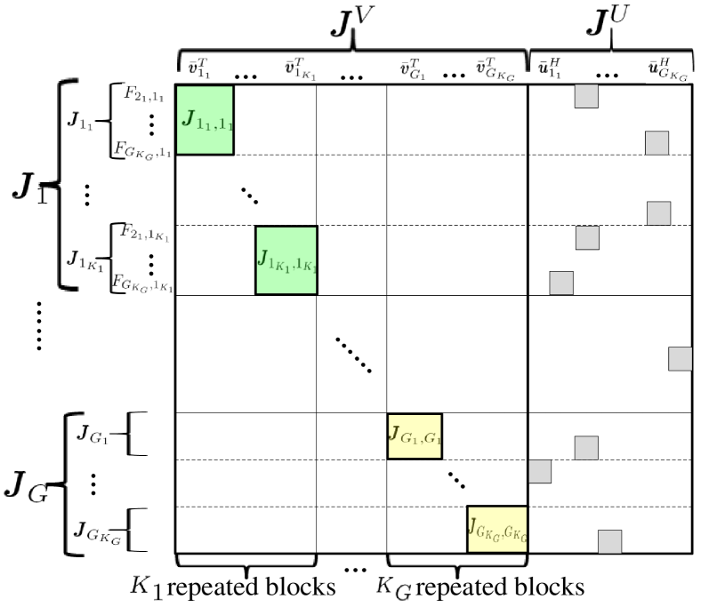
Figure 2: Structure of $\boldsymbol{J}(\bar{\boldsymbol{H}}_{0})$ of MIMO-IBC $\prod_{i=1}^{G}(M_{i}\times\prod_{k=1}^{K_{i}}(N_{i_{k}},1))$.

In the following, we construct an invertible Jacobian matrix with such sparse structure and repeated structure.

Essentially, the existence of an invertible Jacobian matrix implies that all the ICIs in the corresponding network can be eliminated with linear IA, as analyzed with a bipartite graph in [12]. This suggests that in order to construct an invertible Jacobian matrix we need to find a way to assign each of the variables in the transmit and receive vectors to each of the ICIs.

The structure of the Jacobian matrix in Fig. 2 gives rise to the following observation: the transmit variable assignment is not as flexible as the receive variable assignment. Specifically, as shown from the proof of Lemma 3, the repeated structure of $\boldsymbol{J}^{V}(\bar{\boldsymbol{H}}_{0})$ requires that if one transmit vector of BS_j is assigned to avoid the ICI to a user in other cell, the other transmit vectors of BS_j have also to avoid the ICI to the same user. In other words, all the transmit vectors at one BS must avoid generating ICIs to the same user in other cell. This leads to the difficulty to construct an invertible Jacobian matrix for the MIMO-IBC considered in Lemma 3, where the BS can only avoid partial ICIs it generated but it does not know which ICIs it should avoid. By contrast, the receive variable assignment in a MIMO-IBC with $d=1$ is flexible, because $\boldsymbol{J}^{U}(\bar{\boldsymbol{H}}_{0})$ does not have the repeated structure. By applying the result in Lemma 1, $\boldsymbol{J}^{U}(\bar{\boldsymbol{H}}_{0})$ can be set as a sub-matrix of a permutation matrix.

Inspired by this observation, we can first construct $\boldsymbol{J}^{U}(\bar{\boldsymbol{H}}_{0})$, i.e., assign the variables in the receive vector to deal with some ICIs, using the way of perfect matching. Then, we construct $\boldsymbol{J}^{V}(\bar{\boldsymbol{H}}_{0})$ to deal with the remaining ICIs. To circumvent the confliction between allowing the transmit vectors of each BS to avoid different ICIs and ensuring the repeated structure of the Jacobian matrix, we only reserve enough variables in these transmit vectors but do not assign variables to eliminate specific ICIs. Such an idea translates to the following two rules to construct the invertible Jacobian matrix.

• Rule 1: All the elements in $\boldsymbol{J}^{U}(\bar{\boldsymbol{H}}_{0})$ are set as the corresponding elements in $\boldsymbol{D}^{\mathcal{W}}$, where $\boldsymbol{D}^{\mathcal{W}}$ is a permutation matrix obtained from Lemma 1.

• Rule 2: All the elements in $\boldsymbol{J}_{j_{1},j_{1}}^{V}(\bar{\boldsymbol{H}}_{0})$ are set to ensure that its arbitrary $M_{j}-K_{j}$ row vectors are linearly independent, and $\boldsymbol{J}_{j_{l},j_{l}}^{V}(\bar{\boldsymbol{H}}_{0})=\boldsymbol{J}_{j_{1},j_{1}}^{V}(\bar{\boldsymbol{H}}_{0}),~{}l=2,\cdots,K_{j}$ that ensures the repeated structure.

Now we prove that the constructed Jacobian matrix following these rules is invertible. Since $\boldsymbol{J}^{V}(\bar{\boldsymbol{H}}_{0})$ is a block diagonal matrix, the nonzero blocks in different matrices of $\boldsymbol{J}_{j_{l}}^{V}(\bar{\boldsymbol{H}}_{0})$ are non-overlapping. Since the elements in $\boldsymbol{J}^{U}(\bar{\boldsymbol{H}}_{0})$ are set from the permutation matrix $\boldsymbol{D}^{\mathcal{W}}$, there is at most one nonzero element in each column or row of $\boldsymbol{J}^{U}(\bar{\boldsymbol{H}}_{0})$. This indicates that the nonzero elements in different matrices of $\boldsymbol{J}_{j_{l}}^{U}(\bar{\boldsymbol{H}}_{0})$ are also non-overlapping. As a result, the nonzero elements in different blocks of $\boldsymbol{J}_{j_{l}}(\bar{\boldsymbol{H}}_{0})=[\boldsymbol{J}_{j_{l}}^{V}(\bar{\boldsymbol{H}}_{0}),\boldsymbol{J}_{j_{l}}^{U}(\bar{\boldsymbol{H}}_{0})]$ are non-overlapping. Considering the definition in (38), we have

$$\mathrm{rank}\left(\boldsymbol{J}(\bar{\boldsymbol{H}}_{0})\right)=\sum_{j=1}^{G}\sum_{l=1}^{K_{j}}\mathrm{rank}\left(\boldsymbol{J}_{j_{l}}(\bar{\boldsymbol{H}}_{0})\right)$$ (44)

In Rule 1, the perfect matching ensures that there are $\sum_{i=1}^{G}K_{i}-M_{j}$ ones in $\boldsymbol{J}_{j_{l}}^{U}(\bar{\boldsymbol{H}}_{0})$ that are scattered in different rows, and then $\mathrm{rank}(\boldsymbol{J}_{j_{l}}^{U}(\bar{\boldsymbol{H}}_{0}))=\sum_{i=1}^{G}K_{i}-M_{j}$.

Using elementary transformations, we can eliminate $\sum_{i=1}^{G}K_{i}-M_{j}$ row vectors of $\boldsymbol{J}_{j_{l}}^{V}(\bar{\boldsymbol{H}}_{0})$ with nonzero elements and leave $M_{j}-K_{j}$ independent row vectors in $\boldsymbol{J}_{j_{l}}^{V}(\bar{\boldsymbol{H}}_{0})$. In this way, the nonzero elements in $\boldsymbol{J}_{j_{l}}^{U}(\bar{\boldsymbol{H}}_{0})$ and the transformed $\boldsymbol{J}_{j_{l}}^{V}(\bar{\boldsymbol{H}}_{0})$ are located in different rows of $\boldsymbol{J}_{j_{l}}(\bar{\boldsymbol{H}}_{0})$. Therefore, $\mathrm{rank}(\boldsymbol{J}_{j_{l}}^{V}(\bar{\boldsymbol{H}}_{0}))=M_{j}-K_{j}$ and $\mathrm{rank}(\boldsymbol{J}_{j_{l}}(\bar{\boldsymbol{H}}_{0}))=\mathrm{rank}(\boldsymbol{J}_{j_{l}}^{V}(\bar{\boldsymbol{H}}_{0}))+\mathrm{rank}(\boldsymbol{J}_{j_{l}}^{U}(\bar{\boldsymbol{H}}_{0}))=\sum_{i=1,i\neq j}^{G}K_{i}$. After substituting to (44), we have

$$\mathrm{rank}\left(\boldsymbol{J}(\bar{\boldsymbol{H}}_{0})\right)=\sum_{j=1}^{G}\sum_{l=1}^{K_{j}}\sum_{i=1,i\neq j}^{G}K_{i}=\sum_{j=1}^{G}\sum_{i=1,i\neq j}^{G}K_{j}K_{i}$$ (45)

Comparing with (37), we know that $\boldsymbol{J}(\bar{\boldsymbol{H}}_{0})$ is invertible. Now, Theorem 2 is proved. ∎

V Discussion: Proper vs Feasible

In this section, we discuss the connection between the proper and feasibility conditions of the linear IA for MIMO-IBC by analyzing and comparing Theorem 1 and Theorem 2. We also show the relationship of our proved necessary and sufficient conditions with existing results in the literature.

V-A “Proper”=“Feasible”

For a class of MIMO-IBC with configuration $\prod_{i=1}^{G}(M_{i}\times\prod_{k=1}^{K_{i}}(N_{i_{k}},d))$ where $M_{i}\geq K_{i}d$ and $N_{i_{k}}\geq d$, from Theorem 2 we know that when both $M_{i}$ and $N_{i_{k}}$ are divisible by $d$, the MIMO-IBC is feasible if it is proper. This immediately leads to the following conclusion: when $d=1$, a proper MIMO-IBC is always feasible for arbitrary $M_{i}$ and $N_{i_{k}}$.

When $d>1$, since there are too many cases of general MIMO-IBC to describe and analyze, in the sequel we only focus on the symmetric MIMO-IBC. We first show the “proper condition” for the symmetric MIMO-IBC.

Corollary 1

For a symmetric MIMO-IBC with configuration $(M\times(N,d)^{K})^{G}$, the second necessary condition in Theorem 1, i.e., the proper condition in (3), reduces to

$$M+N\geq(GK+1)d$$ (46)

Proof:

See Appendix D. ∎

Note that (46) was also obtained in [15] from counting the total number of variables and equations. However, it was not proposed as the proper condition. From the definition of the proper system in [11], a system is proper iff for every subset of the equations, the number of the variables involved is at least as large as the number of the equations. This means that to prove (46) as the proper condition, we need to check: if (46) satisfies, whether (3) always holds for arbitrary sets $\mathcal{I}\subseteq\mathcal{J}$ and $\mathcal{K}_{i}\subseteq\{1,\cdots,K\}$.

From Theorem 2 and Corollary 1 we know that for a symmetric MIMO-IBC with $M\geq Kd$ and $N\geq d$, when $M$ and $N$ are divisible by $d$, the IA of the symmetric MIMO-IBC will be feasible if the system is proper. Next, we derive from Theorem 2 that for a more general class of symmetric MIMO-IBC, the IA will be feasible if the system is proper.

Corollary 2

For a symmetric MIMO-IBC, when

$$M\geq(K+p)d,~{}N\geq((G-1)K+1-p)d$$

$$\quad\quad\quad\exists p\in\{0,\cdots,(G-1)K\}$$ (47)

the IA is feasible.

Proof:

See Appendix E. ∎

This is the sufficient and necessary condition of the IA feasibility, where $M$ and $N$ are not necessary to be divisible by $d$ or $K$. Since for the symmetric MIMO-IBC the condition that either $M$ or $N$ is divisible by $d$ is one special case of (2), when either $M$ or $N$ is divisible by $d$, the proper symmetric MIMO-IBC is feasible.

In literature, the sufficiency has been proved only for three specific MIMO-IBC systems [4, 9, 19] and for two special classes of MIMO-IC [12, 13].

For the three MIMO-IBC systems with $G=2$, $d=1$, $M=N=K+1$ in [4], with $G=2$, $M=(K+1)d$, $N=Kd$ in [19] and with $G=2$, $M=Kd$, $N=(K+1)d$ in [9], the sufficiency was proved implicitly by proposing closed-form linear IA algorithms. We can see that these configurations satisfy (46) and (2), i.e., the three systems are proper and feasible, which are special cases of our results in Corollary 2.

For the two classes of MIMO-IC in [12, 13], we can extend their results into MIMO-IBC by the following proposition.

Proposition 1

If there exists an invertible Jacobian matrix for a class of MIMO-IC with configuration $\prod_{i=1}^{G}(M_{i}\times N_{i},K_{i})$, there will exist an invertible Jacobian matrix for a class of MIMO-IBC with configuration $\prod_{i=1}^{G}(M_{i}\times\prod_{k=1}^{K_{i}}(N_{i_{k}},1))$.

Proof:

See Appendix F. ∎

According to Proposition 1, the sufficiency proof for the class of MIMO-IC in [12] where either $M$ or $N-d$ is divisible by $d$ can be extended to a class of MIMO-IBC where either $M$ or $N-d$ is divisible by $Kd$, which is a sub-class of those shown in Corollary 2. Similarly, the sufficiency proof for the class of MIMO-IC in [13] where $G\geq 3$ and $M=N$ can be extended to a class of MIMO-IBC where $G\geq 3$ and $M=N+(K-1)d$. It is not hard to show that except for the cases when $(G-1)K$ is odd, all extended cases from [13] are the special cases of those in Corollary 2. When these extended MIMO-IBC systems satisfy the proper condition in (46), they are feasible.

V-B “Proper”$\neq$“Feasible”

For a symmetric MIMO-IBC, the third necessary condition in Theorem 1, i.e., (3), reduces to

$$\max\{pM,~{}qN\}\geq pKd+qd$$ (48)

where $p$ and $q$ were defined after (21).

In a symmetric MIMO-IBC where $M\geq Kd$ and $N\geq d$, when $M$ and $N$ satisfy (46) but do not satisfy (48), the MIMO-IBC is proper but infeasible. However, some conditions in (48) can be derived from (46). To investigate the proper but infeasible region of antenna configuration, we need to find which necessary conditions in (48) are not included in the proper condition.

TABLE I: Necessary conditions other than proper condition for symmetric proper systems

References	Necessary conditions other than proper condition	Corresponding proper but infeasible cases
		Case I	Case II	Other cases except I and II
Corollary 3	$\left\{\begin{array}[]{l}\max\{M,(G-1)KN\}\geq GKd\\ \max\{(G-1)M,N\}\geq((G-1)K+1)d\end{array}\right.,~{}\forall K,G$	$\forall K,G$	$\forall K,G$
[12]∗,[13]∗	$\max\{M,N\}\geq(K+1)d,~{}\forall K,G$		$G=2,\forall K$
[16]	$\left\{\begin{array}[]{l}\max\{M,(L-1)KN\}\geq LKd\\ \max\{(L-1)M,KN\}\geq LKd\end{array}\right.,~{}L=2,\cdots,G,~{}\forall K,G$	$\forall K,G$	$K=1,\forall G$
[9]	$\left\{\begin{array}[]{l}\max\{M,(G-1)N\}\geq(K+G-1)d\\ \max\{(G-1)M,KN\}\geq(K+G-1)d\end{array}\right.,~{}\forall K,G$	$K=1,\forall G$	$K=1,\forall G$
[17],[18]	$\left\{\begin{array}[]{l}\max\{LM,(L+1)N\}\geq(2L+1)d\\ \max\{(L+1)M,LN\}\geq(2L+1)d\end{array}\right.,~{}\forall L\geq 1,\left\{\begin{array}[]{l}K=1\\ G=3\\ \end{array}\right.$	$K=1,G=3$	$K=1,G=3$	$K=1,G=3$
[6]	$\left\{\begin{array}[]{l}\max\{M,(G-1)N\}\geq Gd\\ \max\{(G-1)M,N\}\geq Gd\\ \frac{(G-1)N}{G^{2}-G-1}\geq d,\forall\frac{G-1}{G(G-2)}\geq\frac{M}{N}\geq\frac{G}{G^{2}-G-1}\\ \frac{(G-1)M}{G^{2}-G-1}\geq d,\forall\frac{G-1}{G(G-2)}\geq\frac{N}{M}\geq\frac{G}{G^{2}-G-1}\end{array}\right.,~{}\left\{\begin{array}[]{l}K=1\\ \forall G\\ \end{array}\right.$	$K=1,\forall G$	$K=1,\forall G$	$K=1,\forall G$

Corollary 3

For a symmetric MIMO-IBC where $M\geq Kd$ and $N\geq d$, there exist at least two necessary conditions that are not included in the proper condition as follows

$$\max\{M,(G-1)KN\}\geq GKd$$ (49a)

$$\max\{(G-1)M,N\}\geq((G-1)K+1)d$$ (49b)

which lead to two proper but infeasible cases,

$$\mathrm{Case~{}I:}~{} \left\{\begin{array}[]{c}\max\{M,(G-1)KN\}<GKd\\ M+N\geq(GK+1)d\end{array}\right.$$

$$\mathrm{Case~{}II:}~{} \left\{\begin{array}[]{c}\max\{(G-1)M,N\}<((G-1)K+1)d\\ M+N\geq(GK+1)d\end{array}\right.$$

When $G=2$ and $K=1$, Case I is the same as Case II, otherwise these two cases are different.

Proof:

See Appendix G. ∎

Many necessary conditions other than the proper condition were provided for various MIMO-IC [6, 12, 13, 17, 18, 20] and MIMO-IBC [9, 16]. In [12, 13], a necessary condition of $\max\{M,N\}\geq 2d$ was provided for symmetric MIMO-IC, which is not difficult to be extended into symmetric MIMO-IBC as $\max\{M,N\}\geq(K+1)d$. In [6, 17, 18], the methods to derive the necessary conditions are only applicable for MIMO-IC. Since some of the necessary conditions can be derived from the proper condition, we only compare the corresponding proper but infeasible cases, which can be obtained from the necessary conditions after some regular but tedious derivations. For conciseness, we omit the details of the derivation. In fact, no more than two conditions in [9, 12, 13, 16] cannot be derived from the proper condition, which leads to no more than two proper but infeasible cases.

We list the existing and our extended results in Table I. It is shown that all existing proper but infeasible cases except those in [6, 17, 18] are special cases of Corollary 3.

For the symmetric MIMO-IC, all the necessary conditions in [6, 17, 18] cannot be derived from the proper condition. For the symmetric three-cell MIMO-IC in [17, 18], when $L=1$, the obtained proper but infeasible cases are included in Cases I and II of our results, when $L>1$, their necessary conditions lead to other proper but infeasible cases, where $L$ is an arbitrary positive integer. For the symmetric $G-$cell MIMO-IC in [6], there are four necessary conditions that correspond to four proper but infeasible cases. Two of the cases are included in Cases I and II of our results, but another two cases are not. Consequently, when $K=1$, the necessary conditions in [6, 17, 18] are more general than ours, but the results are only applicable for MIMO-IC.

V-C An example

In Fig. 3, we illustrate the feasible and infeasible regions (i.e., the corresponding system configuration) with an example. The feasible results from Corollary 2 are shown by horizontal lines. The extended results from [12] and from [13] through Proposition 1 are respectively in dash and dot-dash lines. It is shown that all the extended results from [12] and from [13] are special cases of those from Corollary 2 since $(G-1)K$ is even in the example.

The two proper but infeasible cases in Corollary 3 are highlighted with red background. In the proper region, except for the region that has been proved to be feasible in Corollary 2 and that has been proved to be infeasible in Corollary 3, the feasibility of the remaining region is still unknown.

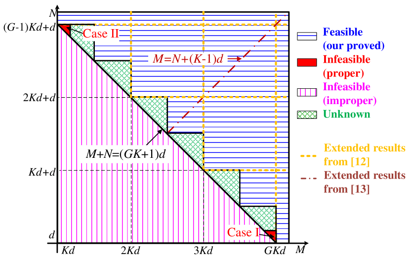
Figure 3: Feasible and infeasible regions of linear IA for the MIMO-IBC supporting overall $GKd$ data streams, $G=4,K=2$, where $(G-1)K$ is even.

VI Conclusion

In this paper, we proposed and proved necessary conditions of linear IA feasibility for general MIMO-IBC with constant coefficients. A necessary condition other than proper condition was posed to ensure the elimination of a kind of irreducible interference. The existence conditions of the reducible and irreducible interference were provided, which depend on the difference in spatial dimension between a base station and multiple users or between a user and multiple base stations.

We proved necessary and sufficient conditions for a special class of MIMO-IBC by finding an invertible Jacobian matrix, which include existing results in literature as special cases. Our analysis showed that when multiple ICIs between one BS and one user can be eliminated either by the BS or by the user, there exists an invertible Jacobian matrix that is a permutation matrix. By contrast, when these ICIs must be eliminated by sharing spatial resources between the BS and the user, the Jacobian matrix cannot be set as a permutation matrix owing to its repeated structure. To deal with the conflicting requirements on the sparse structure and the repeated structure of MIMO-IBC, a general rule to construct an invertible Jacobian matrix was proposed, by exploiting the flexibility of MIMO-IBC in assigning the spatial sources at the users. Finally, we analyzed the feasible, proper but infeasible, and unknown regions in antenna configuration for a proper symmetric MIMO-IBC. The analysis is not applicable to the MIMO-IBC with symbol extension.

Appendix A Proof of Lemma 1

Proof:

The relationship between the equations and variables in (32) can be represented by a bipartite graph, denoted by $C=\left(\mathcal{X},\mathcal{Y},\mathcal{E}\right)$, where $\mathcal{Y}$ is the set of vertices representing the scalar equations, $\mathcal{X}$ is the set of vertices representing the scalar variables, $\mathcal{E}$ is the set of edges and $[Y_{m},X_{n}]\in\mathcal{E}$ iff equation $Y_{m}$ contains variable $X_{n}$, where $X_{m}$ and $Y_{m}$ are the $m$th elements in $\mathcal{X}$ and $\mathcal{Y}$, respectively.

Hall’s theorem [24, Theorem 3.1.11] indicates that in a bipartite graph, a perfect matching exists iff $|N(\mathcal{S})|\geq|\mathcal{S}|,~{}\forall\mathcal{S}\subseteq\mathcal{Y}$, where $N(\mathcal{S})$ is the set of all vertices adjacent to some elements of $\mathcal{S}$. In a general MIMO-IBC with configuration $\prod_{i=1}^{G}(M_{i}\times\prod_{k=1}^{K_{i}}(N_{i_{k}},d_{i_{k}}))$, $|\mathcal{S}|=\sum_{(i,j)\in\mathcal{I}}d_{j}\sum_{k\in\mathcal{K}_{i}}d_{i_{k}}$ and $|N(\mathcal{S})|=\sum_{j:(i,j)\in\mathcal{I}}\left(M_{j}-d_{j}\right)d_{j}+\sum_{i:(i,j)\in\mathcal{I}}\sum_{k\in\mathcal{K}_{i}}\left(N_{i_{k}}-d_{i_{k}}\right)d_{i_{k}}$, therefore, $|N(\mathcal{S})|\geq|\mathcal{S}|$ is actually the proper condition for the MIMO-IBC. Consequently, according to Hall’s theorem we know that when the MIMO-IBC is proper and $L_{v}=L_{e}$, there exists a perfect matching in the bipartite graph.

Denote a perfect matching in $\mathcal{C}$ as $\mathcal{W}$, it is clear that $\mathcal{W}\subseteq\mathcal{E}$. The perfect matching $\mathcal{W}$ can be represented by an adjacency matrix $\boldsymbol{D}^{\mathcal{W}}$, that represents which vertices in one set of a graph are connected to the vertices in the other set. Then, the $(m,n)$th element of $\boldsymbol{D}^{\mathcal{W}}$ is

$$D_{m,n}^{\mathcal{W}}=\left\{\begin{array}[]{ll}1,&~{}\forall[Y_{m},X_{n}]\in\mathcal{W}\\ 0,&~{}\forall[Y_{m},X_{n}]\notin\mathcal{W}\end{array}\right.$$ (A.3)

In the perfect matching, the two sets of vertices have a one-to-one mapping relationship. Therefore, $\boldsymbol{D}^{\mathcal{W}}$ is a permutation matrix such that the elements of $\boldsymbol{D}^{\mathcal{W}}$ satisfy $\sum_{m=1}^{L_{e}}D_{m,n}^{\mathcal{W}}=1$ and $\sum_{n=1}^{L_{e}}D_{m,n}^{\mathcal{W}}=1$.

From (36), we know that the sparse property of Jacobian matrix indicates that the $(m,n)$th element satisfies

$$J_{m,n}=\frac{\partial Y_{m}}{\partial X_{n}}=0, ~{}\forall[Y_{m},X_{n}]\notin\mathcal{E}$$ (A.4)

Since $\mathcal{W}\subseteq\mathcal{E}$, from (A.3) we have $D_{m,n}^{\mathcal{W}}=0,\forall[Y_{m},X_{n}]\notin\mathcal{E}$. Compared with (A.4), we know that $\boldsymbol{D}^{\mathcal{W}}$ has the same sparse structure as the Jacobian matrix for a proper system with $L_{v}=L_{e}$. ∎

Appendix B Proof of Lemma 2

Proof:

When $d_{i_{k}}=d$, and $M_{j}$ and $N_{i_{k}}$ are divisible by $d$, (32) can be further rewritten as

$$\boldsymbol{F}_{i_{k},j_{l}}(\bar{\boldsymbol{H}}_{0})=\bar{\boldsymbol{H}}_{0~{}i_{k},j}^{(2)}\bar{\boldsymbol{V}}_{j_{l}}+\bar{\boldsymbol{U}}_{i_{k}}^{H}\bar{\boldsymbol{H}}_{0~{}i_{k},j_{l}}^{(3)}$$ (B.1)

$$= \sum_{t=1}^{M_{j}/d-K_{j}}\bar{\boldsymbol{H}}_{0~{}i_{k},j}^{(2),t}\bar{\boldsymbol{V}}_{j_{l}(t)}+\sum_{s=1}^{N_{i_{k}}/d-1}\bar{\boldsymbol{U}}^{H}_{i_{k}(s)}\bar{\boldsymbol{H}}_{0~{}i_{k},j_{l}}^{(3),s}=\boldsymbol{0},~{}\forall i\neq j$$

where $\bar{\boldsymbol{V}}_{j_{l}(t)}$ and $\bar{\boldsymbol{H}}_{0~{}i_{k},j}^{(2),t}$ are the $t$th block of size $d\times d$ in $\bar{\boldsymbol{V}}_{j_{l}}$ and $\bar{\boldsymbol{H}}_{0~{}i_{k},j}^{(2)}$, $\bar{\boldsymbol{U}}_{i_{k}(s)}$ and $\bar{\boldsymbol{H}}_{0~{}i_{k},j_{l}}^{(3),s}$ are the $s$th block of size $d\times d$ in $\bar{\boldsymbol{U}}_{i_{k}}$ and $\bar{\boldsymbol{H}}_{0~{}i_{k},j_{l}}^{(3)}$.

Then, from (34c) and (34f), the elements of $\boldsymbol{J}(\bar{\boldsymbol{H}}_{0})$ become

$$\frac{\partial\mathrm{vec}\{\boldsymbol{F}_{i_{k},j_{l}}(\bar{\boldsymbol{H}}_{0})\}}{\partial\mathrm{vec}\{\bar{\boldsymbol{V}}_{m_{n}(t)}\}} =\left\{\begin{array}[]{ll}\bar{\boldsymbol{H}}_{0~{}i_{k},j}^{(2),t}\otimes\boldsymbol{I}_{d},&~{}\forall m_{n}=j_{l}\\ \boldsymbol{0}_{d^{2}},&~{}\forall m_{n}\neq j_{l}\end{array}\right.$$ (B.2c)

$$\frac{\partial\mathrm{vec}\{\boldsymbol{F}_{i_{k},j_{l}}(\bar{\boldsymbol{H}}_{0})\}}{\partial\mathrm{vec}\{\bar{\boldsymbol{U}}^{H}_{m_{n}(s)}\}} =\left\{\begin{array}[]{ll}\boldsymbol{I}_{d}\otimes(\bar{\boldsymbol{H}}_{0~{}i_{k},j_{l}}^{(3),s})^{T},&~{}\forall m_{n}=i_{k}\\ \boldsymbol{0}_{d^{2}},&~{}\forall m_{n}\neq i_{k}\end{array}\right.$$ (B.2f)

where $t=1,\cdots,M_{j}/d-K_{j}$, $s=1,\cdots,N_{i_{k}}/d-1$.

When let $\bar{\boldsymbol{H}}_{0~{}i_{k},j}^{(2),t}=\bar{h}_{0~{}i_{k},j}^{(2),t}\boldsymbol{I}_{d}$ and $\bar{\boldsymbol{H}}_{0~{}i_{k},j_{l}}^{(3),s}=\bar{h}_{0~{}i_{k},j_{l}}^{(3),s}\boldsymbol{I}_{d}$, where $\bar{h}_{0~{}i_{k},j}^{(2),t}$ and $\bar{h}_{0~{}i_{k},j_{l}}^{(3),s}$ are the $(1,1)$th elements of $\bar{\boldsymbol{H}}_{0~{}i_{k},j}^{(2),t}s$ and $\bar{\boldsymbol{H}}_{0~{}i_{k},j_{l}}^{(3),s}$, respectively, we have $\bar{\boldsymbol{H}}_{0~{}i_{k},j}^{(2),t}\otimes\boldsymbol{I}_{d}=\bar{h}_{0~{}i_{k},j}^{(2),t}\boldsymbol{I}_{d^{2}}$ and $\boldsymbol{I}_{d}\otimes\bar{\boldsymbol{H}}_{0~{}i_{K_{i}},j_{l}}^{(3),s}=\bar{h}_{0~{}i_{k},j_{l}}^{(3),s}\boldsymbol{I}_{d^{2}}$. As a result, the Jacobian matrix for a MIMO-IBC with configuration $\prod_{i=1}^{G}(M_{i}\times\prod_{k=1}^{K_{i}}(N_{i_{k}},d))$ can be rewritten as $\boldsymbol{J}(\bar{\boldsymbol{H}}_{0})=\tilde{\boldsymbol{J}}(\bar{\boldsymbol{H}}_{0})\otimes\boldsymbol{I}_{d^{2}}$, where $\tilde{\boldsymbol{J}}(\bar{\boldsymbol{H}}_{0})$ has the same pattern of nonzero elements as the Jacobian matrix for a MIMO-IBC with configuration $\prod_{i=1}^{G}(M_{i}/d\times\prod_{k=1}^{K_{i}}(N_{i_{k}}/d,1))$. Therefore, once an invertible matrix $\tilde{\boldsymbol{J}}(\bar{\boldsymbol{H}}_{0})$ is obtained, an invertible matrix $\boldsymbol{J}(\bar{\boldsymbol{H}}_{0})$ is obtained immediately. Moreover, if $\tilde{\boldsymbol{J}}(\bar{\boldsymbol{H}}_{0})$ is a permutation matrix, $\boldsymbol{J}(\bar{\boldsymbol{H}}_{0})$ is also a permutation matrix. ∎

Appendix C Proof of Lemma 3

Proof:

In a general MIMO-IBC with configuration $\prod_{i=1}^{G}(M_{i}\times\prod_{k=1}^{K_{i}}(N_{i_{k}},d_{i_{k}}))$, for an arbitrary data stream of MS${}_{i_{k}}$, the number of ICIs it experienced is an element in $\phi_{i}$, and the number of variables in its effective receive vector is $N_{i_{k}}-d_{i_{k}}$. When $N_{i_{k}}-d_{i_{k}}\leq\sum_{j=1,j\neq i}^{G}d_{j}$ and $N_{i_{k}}-d_{i_{k}}\notin\phi_{i}$, there will exist one BS (say BS_j) where the number of variables in the effective receive vector of MS${}_{i_{k}}$ is not large enough to cancel all the $d_{j}$ ICIs generated from BS_j, denoted by ${Y}_{1},\cdots,{Y}_{d_{j}}$. When $N_{i_{k}}-d_{i_{k}}>0$, the effective receive vector of MS${}_{i_{k}}$ is able to cancel a part of the ICIs from BS_j, which means that BS_j cannot avoid all the ICIs to the data stream of MS${}_{i_{k}}$ considering $L_{v}=L_{e}$. Consequently, these conditions imply that the $d_{j}$ ICIs from BS_j to the data stream of MS${}_{i_{k}}$ need to be jointly eliminated by BS_j and MS${}_{i_{k}}$, rather than solely by BS_j or MS${}_{i_{k}}$.

We first show the structure of a Jacobian matrix if it is set as a permutation matrix $\boldsymbol{D}^{\mathcal{W}}$. Denote the $t$th variable of the $m$th transmit vector of BS_j as $X_{m(t)}$, where $t=1,\cdots,M_{j}-d_{j}$ and $m=1,\cdots,d_{j}$. If an effective transmit variable $X_{m(t)}$ is assigned to avoid the ICI $Y_{m}$ in the perfect matching, from (A.3), we know that setting $\boldsymbol{J}(\bar{\boldsymbol{H}}_{0})=\boldsymbol{D}^{\mathcal{W}}$ requires $\partial Y_{m}/\partial X_{m(t)}=1$, otherwise $\partial Y_{m}/\partial X_{m(t)}=0$. Since ${Y}_{1},\cdots,{Y}_{d_{j}}$ need to be eliminated by BS_j and MS${}_{i_{k}}$ jointly, a perfect matching (that corresponds a permutation matrix that satisfies the sparse structure) requires that some of $\partial Y_{1}/\partial X_{1(t)},\cdots,\partial Y_{d_{j}}/\partial X_{d_{j}(t)}$ are ones and others are zeros.

According to the repeated structure of the Jacobian matrix shown in (34c) and (35), we have $\partial Y_{1}/\partial X_{1(t)}=\cdots=\partial Y_{d_{j}}/\partial X_{d_{j}(t)}$. As a result, any permutation matrix that satisfies the sparse structure of the Jacobian matrix cannot satisfy its repeated structure. Therefore, there does not exist a Jacobian matrix that is a permutation matrix. ∎

Appendix D Proof of Corollary 1

Proof:

For a symmetric MIMO-IBC, (3) becomes

$$\left(M-Kd\right)K_{\mathrm{T}}+\left(N-d\right)K_{\mathrm{R}}\geq\sum_{(i,j)\in\mathcal{I}}K|\mathcal{K}_{i}|d$$ (D.1)

where $K_{\mathrm{T}}=\sum_{j\in\mathcal{I}_{\mathrm{T}}}K$, $K_{\mathrm{R}}=\sum_{i\in\mathcal{I}_{\mathrm{R}}}|\mathcal{K}_{i}|$, $\mathcal{I}_{\mathrm{T}}=\{j|(i,j)\in\mathcal{I}\}$ and $\mathcal{I}_{\mathrm{R}}=\{i|(i,j)\in\mathcal{I}\}$. $\mathcal{I}_{\mathrm{T}}$ and $\mathcal{I}_{\mathrm{R}}$ denote the index sets of the cells in $\mathcal{I}$ that generate ICI and suffer from the ICI, $K_{\mathrm{T}}$ and $K_{\mathrm{R}}$ are the total numbers of users in the cells with indices in $\mathcal{I}_{\mathrm{T}}$ and $\mathcal{I}_{\mathrm{R}}$, respectively.

Define $\tilde{\mathcal{I}}\triangleq\{(i,j)|i\neq j,~{}\forall j\in\mathcal{I}_{\mathrm{T}},~{}i\in\mathcal{I}_{\mathrm{R}}\}$, it is easy to know $\mathcal{I}\subseteq\tilde{\mathcal{I}}$. Therefore, the right-hand side of (D.1) satisfies

$$\sum_{(i,j)\in\mathcal{I}}K|\mathcal{K}_{i}|d\leq\sum_{(i,j)\in\tilde{\mathcal{I}}}K|\mathcal{K}_{i}|d$$ (D.2)

$$= \sum_{j\in\mathcal{I}_{\mathrm{T}}}K\sum_{i\in\mathcal{I}_{\mathrm{R}},i\neq j}|\mathcal{K}_{i}|=\sum_{i\in\mathcal{I}_{\mathrm{R}}}|\mathcal{K}_{i}|\sum_{j\in\mathcal{I}_{\mathrm{T}},j\neq i}K$$

Since $\mathcal{I}_{\mathrm{T}}\subseteq\{1,\ldots,G\}$, we have $\sum_{i\in\mathcal{I}_{\mathrm{R}}}|\mathcal{K}_{i}|\sum_{j\in\mathcal{I}_{\mathrm{T}},j\neq i}K\leq\sum_{i\in\mathcal{I}_{\mathrm{R}}}|\mathcal{K}_{i}|\sum_{j=1,i\neq j}^{G}K=(G-1)KK_{\mathrm{R}}$. Since $\mathcal{I}_{\mathrm{R}}\subseteq\{1,\ldots,G\}$ and $|\mathcal{K}_{i}|\leq K$, we have $\sum_{j\in\mathcal{I}_{\mathrm{T}}}K\sum_{i\in\mathcal{I}_{\mathrm{R}},i\neq j}|\mathcal{K}_{i}|\leq\sum_{j\in\mathcal{I}_{\mathrm{T}}}K\sum_{i=1,i\neq j}^{G}K=(G-1)KK_{\mathrm{T}}$. After substituting into (D.2), we obtain an upper-bound of the right-hand side of (D.1) as

$$\sum_{(i,j)\in\mathcal{I}}K|\mathcal{K}_{i}|d\leq(G-1)Kd\min\{K_{\mathrm{R}},K_{\mathrm{T}}\}$$ (D.3)

Because $K_{\mathrm{T}}\geq\min\{K_{\mathrm{R}},K_{\mathrm{T}}\}$ and $K_{\mathrm{R}}\geq\min\{K_{\mathrm{R}},K_{\mathrm{T}}\}$, the left-hand side of (D.1) satisfies

$$\left(M-Kd\right)K_{\mathrm{T}}+\left(N-d\right)K_{\mathrm{R}}$$

$$\geq \left(M+N-(K+1)d\right)\min\{K_{\mathrm{R}},K_{\mathrm{T}}\}$$ (D.4)

From (46), we have $M+N-(K+1)d\geq(G-1)Kd$. Substituting this inequity into (D), we obtain a lower-bound of the left-hand side of (D.1) as

$$\left(M-Kd\right)K_{\mathrm{T}}+\left(N-d\right)K_{\mathrm{R}}\geq(G-1)Kd\min\{K_{\mathrm{R}},K_{\mathrm{T}}\}$$ (D.5)

Consider (D.3) and (D.5), we obtain (D.1). ∎

Appendix E Proof of Corollary 2

Proof:

For notation simplicity, we define $M_{p}=(K+p)d$ and $N_{p}=((G-1)K+1-p)d$ here. To prove the MIMO-IBC with configuration $(M\times(N,d)^{K})^{G}$ where $M$ and $N$ satisfy $M\geq M_{p},~{}N\geq N_{p},~{}\exists p$ to be feasible, we first prove its IA to be feasible when $M=M_{p},~{}N=N_{p},~{}\exists p$.

Since $M_{p}+N_{p}=(GK+1)d,~{}\forall p\in\{0,\cdots,(G-1)K\}$, according to Corollary 1, we know that the MIMO-IBC with configuration $(M_{p}\times(N_{p},d)^{K})^{G}$ is proper. Because $M_{p}\geq Kd,~{}N_{p}\geq d$ and both $M_{p}$ and $N_{p}$ are divisible by $d$, according to Theorem 2, the IA for the MIMO-IBC with configuration $(M_{p}\times(N_{p},d)^{K})^{G}$ is feasible. ∎

Appendix F Proof of Proposition 1

Proof:

For conciseness, we use $\boldsymbol{J}_{\mathrm{IBC}}(\bar{\boldsymbol{H}}_{0})$ and $\boldsymbol{J}_{\mathrm{IC}}(\bar{\boldsymbol{H}}_{0})$ to denote the Jacobian matrix of the MIMO-IBC with configuration $\prod_{i=1}^{G}(M_{i}\times\prod_{k=1}^{K_{i}}(N_{i_{k}},1))$ and that of the MIMO-IC with configuration $\prod_{i=1}^{G}(M_{i}\times N_{i},K_{i})$, respectively. To show how to obtain an invertible $\boldsymbol{J}_{\mathrm{IBC}}(\bar{\boldsymbol{H}}_{0})$ from an invertible Jacobian matrix $\boldsymbol{J}_{\mathrm{IC}}(\bar{\boldsymbol{H}}_{0})$, we first show the structure of $\boldsymbol{J}_{\mathrm{IC}}(\bar{\boldsymbol{H}}_{0})$.

In the MIMO-IC, (31) can be rewritten as

$${F}_{i_{k},j_{l}}^{\mathrm{IC}}(\bar{\boldsymbol{H}}_{0})=\bar{\boldsymbol{h}}_{0~{}i_{k},j}^{(2)}\bar{\boldsymbol{v}}_{j_{l}}+\bar{\boldsymbol{u}}_{i_{k}}^{H}\bar{\boldsymbol{h}}_{0~{}i,j_{l}}^{(3)}=0,~{}\forall i\neq j$$ (F.1)

where ${F}_{i_{k},j_{l}}(\cdot)$ represents the ICI from the $l$th data stream transmitted from BS_j to the $k$th data stream received at MS_i.

From (34c), (34f) and (F.1), we can obtain the elements of the Jacobian matrix as follows,

$$\frac{\partial{F}_{i_{k},j_{l}}^{\mathrm{IC}}(\bar{\boldsymbol{H}}_{0})}{\partial\bar{\boldsymbol{v}}_{m_{n}}} =\left\{\begin{array}[]{ll}\bar{\boldsymbol{h}}_{0~{}i_{k},j}^{(2)},&~{}\forall m_{n}=j_{l}\\ \boldsymbol{0}_{1\times(M_{m}-K_{m})},&~{}\forall m_{n}\neq j_{l}\end{array}\right.$$ (F.2c)

$$\frac{\partial{F}_{i_{k},j_{l}}^{\mathrm{IC}}(\bar{\boldsymbol{H}}_{0})}{\partial\bar{\boldsymbol{u}}^{H}_{m_{n}}} =\left\{\begin{array}[]{ll}(\bar{\boldsymbol{h}}_{0~{}i,j_{l}}^{(3)})^{T},&~{}\forall m_{n}=i_{k}\\ \boldsymbol{0}_{1\times(N_{m}-K_{m})},&~{}\forall m_{n}\neq i_{k}\end{array}\right.$$ (F.2f)

In (F.2c) and (F.2f), one can see that the nonzero elements satisfy

$$\frac{\partial F_{i_{k},j_{1}}^{\mathrm{IC}}(\bar{\boldsymbol{H}}_{0})}{\partial\bar{\boldsymbol{v}}_{j_{1}}}=\cdots=\frac{\partial{F}_{i_{k},j_{K_{j}}}^{\mathrm{IC}}(\bar{\boldsymbol{H}}_{0})}{\partial\bar{\boldsymbol{v}}_{j_{K_{j}}}}=\bar{\boldsymbol{h}}_{0~{}i_{k},j}^{(2)}$$ (F.3a)

$$\frac{\partial{F}_{i_{1},j_{l}}^{\mathrm{IC}}(\bar{\boldsymbol{H}}_{0})}{\partial\bar{\boldsymbol{u}}^{H}_{i_{1}}}=\cdots=\frac{\partial{F}_{i_{K_{i}},j_{l}}^{\mathrm{IC}}(\bar{\boldsymbol{H}}_{0})}{\partial\bar{\boldsymbol{u}}^{H}_{i_{K_{i}}}}=\bar{\boldsymbol{h}}_{0~{}i,j_{l}}^{(3)}$$ (F.3b)

Comparing (39c) and (39f) with (F.2c) and (F.2f), it is easy to find that when $N_{i_{k}}-1=N_{i}-K_{i},~{}\forall i,k$, $\boldsymbol{J}_{\mathrm{IBC}}(\bar{\boldsymbol{H}}_{0})$ has the same nonzero element pattern with $\boldsymbol{J}_{\mathrm{IC}}(\bar{\boldsymbol{H}}_{0})$. Moreover, comparing (40a) and (F.3a), we can see that the repeated nonzero elements in $\boldsymbol{J}^{V}_{\mathrm{IBC}}(\bar{\boldsymbol{H}}_{0})$ have the same pattern as those in $\boldsymbol{J}^{V}_{\mathrm{IC}}(\bar{\boldsymbol{H}}_{0})$. By contrast, comparing (40b) and (F.3b), we can see that the nonzero elements of $\boldsymbol{J}^{U}_{\mathrm{IBC}}(\bar{\boldsymbol{H}}_{0})$ are generic but those of $\boldsymbol{J}^{U}_{\mathrm{IC}}(\bar{\boldsymbol{H}}_{0})$ are not since they are repeated. This suggests that the elements of $\boldsymbol{J}_{\mathrm{IBC}}(\bar{\boldsymbol{H}}_{0})$ are more flexible to be set into any value than that of $\boldsymbol{J}_{\mathrm{IC}}(\bar{\boldsymbol{H}}_{0})$. Hence, if there exists an invertible $\boldsymbol{J}_{\mathrm{IC}}(\bar{\boldsymbol{H}}_{0})$, we can obtain an invertible $\boldsymbol{J}_{\mathrm{IBC}}(\bar{\boldsymbol{H}}_{0})$ by setting $\boldsymbol{J}_{\mathrm{IBC}}(\bar{\boldsymbol{H}}_{0})=\boldsymbol{J}_{\mathrm{IC}}(\bar{\boldsymbol{H}}_{0})$. ∎

Appendix G Proof of Corollary 3

Proof:

If $M$ and $N$ do not satisfy (48), we have $\max\{pM,~{}qN\}<pKd+qd$, i.e., $pM<pKd+qd$ and $qN<pKd+qd$. Considering $M+N\geq(GK+1)d$ in (46), we can obtain the proper but infeasible region, which satisfies

$$M<\frac{pK+q}{p}d,~{}N<\frac{pK+q}{q}d$$ (G.1a)

$$M+N\geq(GK+1)d$$ (G.1b)

From (G.1a), we have $M+N<(pK+q)(1/p+1/q)d$. From (G.1b), we have $M+N\geq(GK+1)d$. Therefore, only if $(pK+q)(1/p+1/q)>GK+1$, the proper but infeasible region will not be empty. It is not hard to show that in the nonempty region, the values of $p,q$ need to satisfy the following quadratic inequality,

$$\Delta\triangleq K\left(\frac{p}{q}\right)^{2}-(G-1)K\frac{p}{q}+1>0$$ (G.2)

$\Delta$ is a convex function. Therefore, if (G.2) does not hold when the value of $p/q$ achieves its minimum or maximum, it will not hold for other values of $p$ and $q$. To find the cases that are proper but infeasible, we first check whether (G.2) is satisfied when $p/q$ achieves its minimum or maximum.

Since in (3), $\mathcal{I}_{\mathrm{A}},\mathcal{I}_{\mathrm{B}}\subseteq\{1,\cdots,G\}$ and $\mathcal{I}_{\mathrm{A}}\cap\mathcal{I}_{\mathrm{B}}=\varnothing$, we have $\mathcal{I}_{\mathrm{A}}\cup\mathcal{I}_{\mathrm{B}}\subseteq\{1,\cdots,G\}$ and $\mathcal{I}_{\mathrm{A}}\cap\mathcal{I}_{\mathrm{B}}=\varnothing$. Therefore, $|\mathcal{I}_{\mathrm{A}}|\leq G-1$, $|\mathcal{I}_{\mathrm{B}}|\leq G-1$ and $|\mathcal{I}_{\mathrm{A}}|+|\mathcal{I}_{\mathrm{B}}|\leq G$. From the definition of $p$ and $q$ after (21), we can derive that,

$$\left\{\begin{array}[]{c}1\leq p\leq G-1,~{}1\leq q\leq(G-1)K\\ Kp+q\leq GK\end{array}\right.$$ (G.5)

From (G.5), it is easy to show that when $p=1,~{}q=(G-1)K$, $p/q=1/((G-1)K)$ achieves the minimum, while when $p=(G-1),~{}q=1$, $p/q=(G-1)$ is the maximum.

When $p=1,~{}q=(G-1)K$, we have $\Delta=1/((G-1)^{2}K)$. Hence, (G.2) holds for all $G,K$. Substituting the values of $p,~{}q$ into (48), we have $\max\{M,(G-1)KN\}\geq GKd$, i.e., (49a), which is one necessary condition that cannot be derived from the proper condition.

When $p=(G-1),~{}q=1$, we have $\Delta=1>0$. Consequently, (G.2) still holds for all $G,K$. Substituting the values of $p,~{}q$ into (48), we have $\max\{(G-1)M,N\}\geq((G-1)K+1)d$, i.e., (49b), which is another necessary condition that cannot be derived from the proper condition. ∎

Tingting Liu (S’09–M’11) received the B.S. and Ph.D. degrees in signal and information processing from Beihang University, Beijing, China, in 2004 and 2011, respectively. From December 2008 to January 2010, she was a Visiting Student with the School of Electronics and Computer Science, University of Southampton, Southampton, U.K. She is currently a Postdoctoral Research Fellow with the School of Electronics and Information Engineering, Beihang University. Her research interests include wireless communications and signal processing, the degrees of freedom (DoF) analysis and interference alignment transceiver design in interference channels, energy efficient transmission strategy design and Joint transceiver design for multicarrier and multiple-input multiple-output communications. She received the awards of the 2012 Excellent Doctoral Thesis in Beijing and the 2012 Excellent Doctoral Thesis in Beihang University.

Chenyang Yang (SM’08) received the M.S.E and Ph.D. degrees in electrical engineering from Beihang University (formerly Beijing University of Aeronautics and Astronautics), Beijing, China, in 1989 and 1997, respectively. She is currently a Full Professor with the School of Electronics and Information Engineering, Beihang University. She has published various papers and filed many patents in the fields of signal processing and wireless communications. Her recent research interests include network MIMO (CoMP, coordinated multi-point), energy efficient transmission (GR, green radio) and interference alignment. Prof. Yang was the chair of Beijing chapter of IEEE Communications Society during 2008 to 2012. She has served as a Technical Program Committee Member for many IEEE conferences, such as the IEEE International Conference on Communications and the IEEE Global Telecommunications Conference. She currently serves as an Associate Editor for IEEE Transactions on Wireless Communications, the Membership Development Committee Chair of Asia Pacific Board of IEEE Communications Society, an Associate Editor-in-Chief of the Chinese Journal of Communications, and an Associate Editor-in-Chief of the Chinese Journal of Signal Processing. She was nominated as an Outstanding Young Professor of Beijing in 1995 and was supported by the First Teaching and Research Award Program for Outstanding Young Teachers of Higher Education Institutions by Ministry of Education (P.R.C. “TRAPOYT”) during 1999 to 2004.

References

• [1] M. K. Karakayali and G. J. Foschini and R. A. Valenzuela, “Network coordination for spectrally efficient communications in cellular systems”, IEEE Wireless Commu., vol. 13, no. 4, pp. 56–61. Aug. 2006.
• [2] S. A. Jafar, “Interference alignment - A new look at signal dimensions in a communication network,” FNT in Communications and Information Theory, vol. 7, no. 1, pp. 1–136, 2010.
• [3] V. R. Cadambe and S. A. Jafar, “Interference alignment and degrees of freedom of the $K$-user interference channel,” IEEE Trans. Inf. Theory, vol. 54, no. 8, pp. 3425–3441, Aug. 2008.
• [4] C. Suh, M. Ho and D.N.C. Tse, “Downlink Interference Alignment,” IEEE Trans. Commun., vol. 59, no. 9, pp. 2616–2626, Sep. 2011.
• [5] S. A. Jafar and M. J. Fakhereddin, “Degrees of freedom for the MIMO interference channel,” IEEE Trans. Inf. Theory, vol. 53, no. 7, pp. 2637–2642, Jul. 2007.
• [6] C. Wang, H. Sun, and S. A. Jafar, “Genie chains and the degrees of freedom of the K-user MIMO interference channel,” in Proc. IEEE ISIT, Jul. 2012.
• [7] S.-H. Park and I. Lee, “Degrees of freedom of multiple broadcast channels in the presence of inter-cell interference,” IEEE Trans. Commun., vol. 59, no. 5, pp. 1481–1487, May 2011.
• [8] J. Kim, S.-H. Park, H. Sung, and I. Lee, “Spatial multiplexing gain for two interfering MIMO broadcast channels based on linear transceiver,” IEEE Trans. Wireless Commun., vol. 9, no. 10, pp. 3012–3017, Oct. 2010.
• [9] T. Kim, D. J. Love, B. Clerckx, and D. Hwang, “Spatial degrees of freedom of the multicell MIMO multiple access channel,” in Proc. IEEE GLOBECOM, Dec. 2011.
• [10] K. Gomadam, V. R. Cadambe, and S. A. Jafar, “Approaching the capacity of wireless networks through distributed interference alignment,” in Proc. IEEE GLOBECOM, Dec. 2008.
• [11] C. M. Yetis, T. Gou, S. A. Jafar, and A. H. Kayran, “On feasibility of interference alignment in MIMO interference networks,” IEEE Trans. Signal Process., vol. 58, no. 9, pp. 4771–4782, Sep. 2010.
• [12] M. Razaviyayn, L. Gennady, and Z. Luo, “On the degrees of freedom achievable through interference alignment in a MIMO interference channel,” IEEE Trans. Signal Process., vol. 60, no. 2, pp. 812-821, Feb. 2012.
• [13] G. Bresler, D. Cartwright, and D. Tse, Settling the feasibility of interference alignment for the MIMO interference channel: the symmetric square case, arXiv:1104.0888v1 [cs.IT], Apr. 2011.
• [14] B. Zhuang, R. A. Berry, and M. L. Honig, “Interference alignment in MIMO cellular networks,” in Proc. IEEE ICASSP, May 2011.
• [15] Y. Ma, J. Li, R. Chen, and Q. Liu, “On feasibility of interference alignment for L-cell constant cellular interfering networks,” IEEE Commun. Lett., vol. 16, no. 5, pp. 714–716, May 2012.
• [16] M. Guillaud and D. Gesbert, “Interference alignment in partially connected interfering multiple-access and broadcast channels,” in Proc. IEEE GLOBECOM, Dec. 2011.
• [17] C. Wang, T. Gou, S. A. Jafar, Subspace Alignment Chains and the Degrees of Freedom of the Three-User MIMO Interference Channel, arXiv:1109.4350v1 [cs.IT], Sep. 2011.
• [18] G. Bresler, D. Cartwright, and D. Tse, “Geometry of the 3-user MIMO interference channel,” in Proc. Allerton, Sep. 2011.
• [19] W. Shin, N. Lee, J.-B. Lim, C. Shin, and K. Jang, “On the design of interference alignment scheme for two-cell MIMO interfering broadcast channels,” IEEE Trans. Wireless Commun., vol. 10, no. 2, pp. 437–442, Feb. 2011.
• [20] L. Ruan, V. K. N. Lau, and M. Z. Win, “The feasibility conditions of interference alignment for MIMO interference networks,” IEEE Trans. Signal Process., early access, 2013.
• [21] O. Gonzalez, I. Santamaria, and C. Beltran, “A general test to check the feasibility of linear interference alignment,” in Proc. IEEE ISIT, Jul. 2012.
• [22] M. Gilli, M. Garbely, “Matchings, covers, and Jacobian matrices,” Journal of Economic Dynamics and Control, vol. 20, no. 9–10, pp. 1541–1556, Sep. 1996.
• [23] D. Meyer, Matrix analysis and applied linear algebra.  Philadelphia, PA: SIAM 2000.
• [24] D. B. West, Introduction to Graph Theory, 2nd ed.  Upper Saddle River, NJ: Prentice-Hall, 2001.